Pyramid Diffusion Models For Low-light Image Enhancement
Abstract
Recovering noise-covered details from low-light images is challenging, and the results given by previous methods leave room for improvement. Recent diffusion models show realistic and detailed image generation through a sequence of denoising refinements and motivate us to introduce them to low-light image enhancement for recovering realistic details. However, we found two problems when doing this, i.e., 1) diffusion models keep constant resolution in one reverse process, which limits the speed; 2) diffusion models sometimes result in global degradation (e.g., RGB shift). To address the above problems, this paper proposes a Pyramid Diffusion model (PyDiff) for low-light image enhancement. PyDiff uses a novel pyramid diffusion method to perform sampling in a pyramid resolution style (i.e., progressively increasing resolution in one reverse process). Pyramid diffusion makes PyDiff much faster than vanilla diffusion models and introduces no performance degradation. Furthermore, PyDiff uses a global corrector to alleviate the global degradation that may occur in the reverse process, significantly improving the performance and making the training of diffusion models easier with little additional computational consumption. Extensive experiments on popular benchmarks show that PyDiff achieves superior performance and efficiency. Moreover, PyDiff can generalize well to unseen noise and illumination distributions. Code and supplementary materials are available at https://github.com/limuloo/PyDIff.git.
1 Introduction
Low-light images suffer from noise bursts, and recovering ideal normal-light images from them is a long-studied problem. Thanks to the development of deep learning, many effective methods have been proposed. LLNet Lore et al. 2017 and SID Chen et al. 2018 show the power of neural networks by training them on lots of paired data. According to the Retinex theory Land 1977, KIND Zhang et al. 2019 and RetinexNet Wei et al. 2018 decompose the illumination and reflectance map through a well-designed loss. To handle this highly ill-posed problem, LLFLOW Wang et al. 2022 introduces normalizing flow models Kingma and Dhariwal 2018 to low-light image enhancement.

Although the above methods have made significant progress in low-light image enhancement, noise-covered details restored by them can be further enhanced. As shown in Fig. 1(a), previous methods often lead to blurred details and distorted colors. Diffusion models Ho et al. 2020; Song et al. 2020b have recently shown their talents in image generation, which can generate more realistic details through a sequence of refinements. Therefore, we introduce diffusion models to low-light image enhancement for better restoring noise-covered details, as shown in Fig. 1(a).
When introducing diffusion models to low-light image enhancement, we found two problems, as demonstrated in Fig. 1(b). 1) The resolution is constant in one reverse process, which limits the speed. 2) Diffusion models result in global degradation similar to the RGB shift we analyze in Fig. 5.
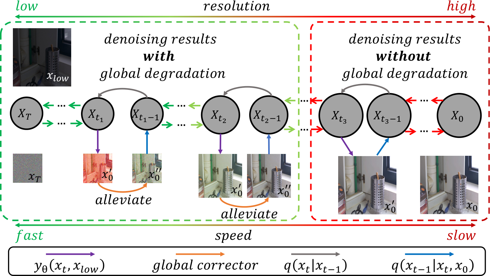
To solve these problems, we propose a Pyramid Diffusion model (PyDiff) for low-light image enhancement. As shown in Fig. 1(c), PyDiff uses a novel pyramid diffusion method to sample images in an efficient pyramid resolution style (i.e., progressively increasing resolution in one reverse process). Performing noisier sampling at lower resolution makes the reverse process faster and provides PyDiff with a larger inception field, which benefits global information recovery. Moreover, we analyze the cause of global degradation (Fig. 5) and argue that denoising networks are hard to treat global degradation as part of the noise and correct it during denoising since the reverse process is biased to eliminate Gaussian noise. To alleviate the global degradation that denoising networks can not notice, PyDiff performs sampling with a global corrector. With little additional computational consumption, the global corrector significantly improves the performance and makes the training of diffusion models easier.
We conduct extensive experiments on two popular benchmarks (i.e., LOL Wei et al. 2018 and LOLV2 Yang et al. 2021) to validate the effectiveness and efficiency of PyDiff. Experimental results show that PyDiff achieves superior performance quantitatively and qualitatively under various scenarios. Compared to the previous state-of-the-art (SOTA) method LLFLOW, which also requires iterative refinements, PyDiff significantly outperforms LLFLOW with a speed of nearly faster. In particular, when dealing with unseen noise distributions, PyDiff significantly outperforms other SOTA competitors, e.g., 10 points (SSIM) higher than the second place (NE Jin et al. 2022). When handling unseen illumination distributions, PyDiff also gives competitive results, demonstrating our generalization ability further.
Our contributions can be summarized below:
- •
To the best of our knowledge, we are the first to introduce diffusion models to low-light image enhancement and achieve SOTA. Using a novel pyramid diffusion method, PyDiff is nearly twice as fast as the previous SOTA method LLFLOW.
- •
We propose a global corrector to alleviate the global degradation that occurs in the reverse process. This significantly improves the performance and makes the training of diffusion models easier with little additional computational consumption.
- •
Experiments on popular benchmarks show that PyDiff achieves new SOTA performance, and PyDiff can generalize well to unseen noise and illumination distributions.
2 Related Work
2.1 Low-light image enhancement
Low-light image enhancement has been studied for a long time, with numerous deep learning-based approaches proposed. LLNet Lore et al. 2017 and SID Chen et al. 2018 collect lots of low/normal-light image pairs to train the network. For getting illumination and reflectance maps Land 1977, RetinexNet Wei et al. 2018, KIND Zhang et al. 2019, and KIND++ Zhang et al. 2021 carefully design the loss to train a decomposition network. EnlightenGAN Jiang et al. 2021, ZeroDCE Guo et al. 2020, and NE Jin et al. 2022 propose effective unsupervised methods which do not require paired data. BREAD Guo and Hu 2022 decouples the entanglement of noise and color distortion. Some works Fan et al. 2022a; Cui et al. 2022; Kim et al. 2021 have brought performance improvements by designing novel and efficient networks. LLFLOW Wang et al. 2022 models this ill-posed problem via a normalizing flow model Dinh et al. 2016; Kingma and Dhariwal 2018. Although the above methods have made significant progress in low-light image enhancement, noise-covered details restored by them can be further enhanced. This paper introduces diffusion models He et al. 2020 to low-light image enhancement for better recovering the details.
2.2 Diffusion models
Diffusion Models Ho et al. 2020; Song et al. 2020b present high-quality image synthesis results recently. However, they typically require a high number of iterations, resulting in slow performance. A number of training-free samplers Song et al. 2020a; Nichol and Dhariwal 2021; Bao et al. 2022; Lu et al. 2022 have been proposed that can achieve comparable results with fewer denoising iterations. To achieve conditional generation, Guided-Diffusion Dhariwal and Nichol 2021 samples with classifier guidance, while our PyDiff concatenates noisy images with source images to guide denoising like some low-level vision methods Saharia et al. 2022b; Saharia et al. 2022a; Whang et al. 2022.
To generate high-resolution images more efficiently, some works Saharia et al. 2022b; Ho et al. 2022; Fan et al. 2022b use multiple diffusion models to achieve cascaded high-resolution image synthesis, while LDM Rombach et al. 2022 makes reverse processes situated within the image encoder’s latent space. In one reverse process, the above methods perform sampling at a constant resolution style, limiting the speed. In this paper, PyDiff uses a pyramid diffusion method to achieve faster speed and a global corrector to ensure the sample quality for low-light image enhancement.
3 Background: Denoising Diffusion Probabilistic Models
The Denoising Diffusion Probabilistic Model Ho et al. 2020; Song et al. 2020a is a latent variable model specified by a T-step Markov chain. It starts with a given data distribution and repeatedly adds Gaussian noise according to as follows:
| (1) |
where , and . Using the notation , the marginal distribution can be expressed as follows:
| (2) |
When is close to 0, the defined forward process will transform this data distribution into an isotropic Gaussian distribution.
In practical applications, the reverse process of diffusion models is used more often, which converts an isotropic Gaussian distribution to a target data distribution. It is worth mentioning that is hard to estimate while is tractable. We can derive the posterior distribution of given with some algebraic manipulation:
| (3) | ||||
| (4) | ||||
| (5) |
where . We have no during testing, but we can calculate its approximate value according to Eq. (2):
| (6) |
where is the predicted noise derived from the denoising network, and is an approximation of calculated according to . Furthermore, we update Eq. (3) as follows:
| (7) |

When it comes to image-to-image translation, Saharia et al. 2022a; Saharia et al. 2022b; Choi et al. 2021 make the reverse process conditional on an input signal. Specifically, when we need to translate to (e.g., low-light image to normal-light image), we update Eq. (6) as follow:
| (8) |
4 Methods
This section presents PyDiff, an effective and efficient method for low-light image enhancement. First of all, we describe the motivation for designing PyDiff. Secondly, we introduce our proposed pyramid diffusion, which significantly improves the inference speed without any performance degradation. Furthermore, we present our proposed global corrector, which alleviates the global degradation that may occur in the reverse process of the diffusion models. Finally, we describe the training and sampling procedures of PyDiff.

4.1 Motivation
Reason for Using Diffusion Models. Diffusion models Ho et al. 2020; Song et al. 2020b have recently shown their talents in image generation, which can generate more realistic details through a sequence of refinements. Therefore, we introduce diffusion models to low-light image enhancement for better restoring noise-covered details.
Shortcomings of Diffusion Models. Diffusion models have often been criticized for their slow inference speed. Many methods Song et al. 2020a; Nichol and Dhariwal 2021; Ho et al. 2022; Saharia et al. 2022b have been proposed to accelerate the reverse process of diffusion models. However, they still suffer from one drawback: the resolution or feature dimension is invariant in one reverse process of diffusion models, which limits the speed.
Constant Resolution is Not Necessary. Taking resolution as an example, we note that constant resolution is not necessary for one reverse process. Fig. 3(a) indicates that the first half of the reverse process can be performed at a lower resolution, which does not affect the details generated at the end.
The Effect of Noisy Sampling. Furthermore, Fig. 3(b) shows that if global degradation (e.g., RGB shift) occurs in the first half (i.e., sampling result has more noise) of the reverse process, the second half (i.e., sampling result has less noise) will not be able to correct it. Fig. 3 demonstrates that noisy sampling (e.g., sampling in the first half of inverse processes) in diffusion models usually does not affect the final details, mainly recovering global information such as brightness and hue. Therefore, PyDiff can perform noisier sampling at a lower resolution while ensuring the global information can be recovered correctly.
4.2 Pyramid Diffusion
As shown in Fig. 2, PyDiff uses a novel pyramid diffusion method to iterate in a pyramid resolution style. Performing nosier sampling at a lower resolution can make the reverse process faster and provide the network with a larger receptive field, which is beneficial for recovering global information. In this section, we introduce the proposed pyramid diffusion.
Downsampling Schedule. Similar to the noise schedule in diffusion models, pyramid diffusion defines a downsampling schedule , which means that the ith sampling will be performed at the resolution downsampled with a scale factor . While to get bigger and bigger noise, to get lower and lower resolution.
Forward Process. For the forward process, pyramid diffusion updates the Eq. (1) in diffusion models as follows:
| (9) |
where means downsampling with a scale factor of . The marginal distribution can be expressed as follows:
| (10) |
Reverse Process. In the case of , we can derive from according to Eq. (7). However, this is no longer applicable in the case of since differences in resolution. As shown in Fig. 4(a), can serve as at noisy sampling (i.e., Larger matches noisier sampling), where means upsampling with a scale factor of . Therefore, with well-scheduled and , we can take as . According to Eq. (10), we can further add noise to for deriving . Adding noise through such a method leads to inconsistency between and . However, this inconsistency has little impact on noisy sampling, which is primarily concerned with recovering global information. To summarize, the posterior distribution of pyramid diffusion can be expressed as follows:
| (11) |
Position Encoding. Pyramid diffusion requires one network to process images of multiple resolutions. As the main operator of the denoising network Ho et al. 2020, convolution kernels cannot perceive the change of resolution. We consider using position encoding to guide the network. For an image with a resolution of , its coordinates are , where , and . After normalizing and , we apply sinusoidal positional encoding of them to guide the network. Specifically, the position encoding is expressed as:
| (12) |
Convolution kernels have a constant receptive field. When dealing with images downsampled with a scale factor of , the range of position encoding perceived by convolution kernels will be correspondingly expanded by times, which may tell convolution kernels the change of resolution.

4.3 Global Corrector
As shown in Fig. 2, PyDiff uses the global corrector to alleviate global degradation in reverse processes. The global corrector can significantly improve performance with little additional computational consumption. In this section, we introduce the proposed global corrector.
Global Degradation. When applying diffusion models to low-light image enhancement, we found them sometimes result in significant global degradation, as shown in Fig. 5(a). This global degradation looks like a shift in the RGB channels, similar to the RGB shift shown in Fig. 3(b).
Cause of Global Degradation. Looking back on Eq. (6), we can rewrite it as follows:
| (13) | ||||
| (14) |
where is the actual noise in , and is the error between and . We found that there is a coefficient in front of the error . When is relatively large, this coefficient will also be large, as shown in Fig. 4(b). As demonstrated in Fig. 5(b), the original error is small, but the coefficient enlarges the error and leads to an obvious RGB shift (e.g., a significant gain in the R channel). As shown in Fig. 5(a), the denoising network treats the image under global degradation as usual and only performs its denoising duties, which can not eliminate the global degradation.
Design of Global Corrector. We add a global corrector to alleviate the global degradation that denoising networks can not notice. The design of the global corrector needs to meet the following requirements: 1) The global corrector should alleviate global degradation while preserving generated edges and textures. 2) The global corrector is lightweight and fast. Inspired by CSRNet He et al. 2020, we design an efficient global corrector that performs pixel-independent retouching based on global conditions. Please refer to the supplementary materials for the specific design of the global corrector. To sample with a global corrector, we update Eq. (7) as follows:
| (15) |
where means using the global corrector to alleviate the global degradation in . Fig. 5(c) shows that the global corrector can alleviate global degradation while maintaining generated edges and textures.
Correction Threshold. As shown in Fig. 4(b), the amplification factor will gradually decrease to 0 as t decreases. When the amplification factor is small enough, it will no longer amplify the error of the denoising network. Therefore, We set a correction threshold , and the global corrector is needed only when the . We set .
4.4 Training and Sampling
To better demonstrate the overall framework of our PyDiff, we omit some details (e.g., position encoding) when describing the algorithm.
Training. Algorithm 1 shows the specific training procedure of the proposed PyDiff. The global corrector aims to alleviate the global degradation that the denoising network cannot notice, and it will not impact the denoising network.
Sampling. Algorithm 2 shows the specific sampling procedure of the proposed PyDiff. PyDiff can be easily combined with DDIM Song et al. 2020a or DDPM+ Nichol and Dhariwal 2021 to achieve further speedup.
Training Loss. As described in algorithm 1, we use the simple L1 loss to optimize the denoising network and global corrector without additional optimization objectives.
5 Experiments
| Input | IAT | KIND | KIND++ | BREAD | NE | HWMNet | LLFLOW | PyDiff | Reference |
|---|---|---|---|---|---|---|---|---|---|
 |
 |
 |
 |
 |
 |
 |
 |
 |
 |
| Input | IAT | KIND | KIND++ | BREAD | NE | HWMNet | LLFLOW | PyDiff | Reference |
|---|---|---|---|---|---|---|---|---|---|
 |
 |
 |
 |
 |
 |
 |
 |
 |
 |
 |
 |
 |
 |
 |
 |
 |
 |
 |
 |
| Methods | PSNR | SSIM | LPIPS |
|---|---|---|---|
| Zero-DCE Guo et al. 2020 | |||
| EnlightenGAN Jiang et al. 2021 | |||
| KinD Zhang et al. 2019 | |||
| KinD++ Zhang et al. 2021 | |||
| RCTNet Kim et al. 2021 | |||
| Bread Guo and Hu 2022 | |||
| NE Jin et al. 2022 | |||
| IAT Cui et al. 2022 | |||
| HWMNet Fan et al. 2022a | |||
| LLFLOW Wang et al. 2022 | |||
| PyDiff (ours) | 27.09 | 0.93 | 0.10 |
5.1 Setup
Dataset. We conduct experiments on LOL Wei et al. 2018 and LOLV2 Yang et al. 2021 datasets. The LOLV2 dataset contains two parts, REAL and SYNC. REAL PART has noise distributions not present in the LOL dataset, and SYNC PART has illumination distributions not present in the LOL dataset. For supervised learning methods involved in comparison, we use their pre-trained model only trained on the LOL dataset. Correspondingly, we train PyDiff only on the LOL dataset too. For unsupervised learning methods, we use their released pre-trained models no matter how they train.
Schedules. First of all, we set . For the noise schedule, we decrease linearly from to . For the downsampling schedule, our default setting is to set and , and we will experiment with more schedules in ablation studies.
Training. We set the patch size to and the batch size to . We use the Adam optimizer with an initial learning rate of for 320k iterations and halve the learning rate at 50k, 75k, 100k, 150k, and 200k. The optimizer does not use weight decay. We complete training on two NVIDIA GeForce RTX 3090s.
Evaluation. Combined with DDIM Song et al. 2020a, PyDiff requires only 4 iterations to obtain results comparable to other SOTA methods.
Other Details. The reverse process is conditional on low-light images , low-light images after histogram equalization , and position encoding . We use the method of concatenating to achieve conditional sampling Saharia et al. 2022b; Saharia et al. 2022a. During training, we swap the concatenating order of and with a probability of 0.5. Please refer to the supplementary materials for model configuration and details of the global corrector.
| Methods | PSNR | SSIM | LPIPS |
|---|---|---|---|
| Zero-DCE Guo et al. 2020 | |||
| KinD Zhang et al. 2019 | |||
| KinD++ Zhang et al. 2021 | |||
| NE Jin et al. 2022 | |||
| IAT Cui et al. 2022 | |||
| Bread Guo and Hu 2022 | |||
| HWMNet Fan et al. 2022a | |||
| LLFLOW Wang et al. 2022 | |||
| PyDiff (ours) | 24.01 | 0.876 | 0.23 |
| Methods | PSNR | SSIM | LPIPS |
|---|---|---|---|
| KIND Zhang et al. 2019 | |||
| KIND++ Zhang et al. 2021 | |||
| IAT Cui et al. 2022 | |||
| Bread Guo and Hu 2022 | |||
| HWMNet Fan et al. 2022a | |||
| LLFLOW Wang et al. 2022 | 0.22 | ||
| PyDiff (ours) | 19.60 | 0.878 | 0.22 |
5.2 Comparsion with SOTA Methods
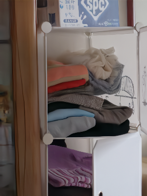
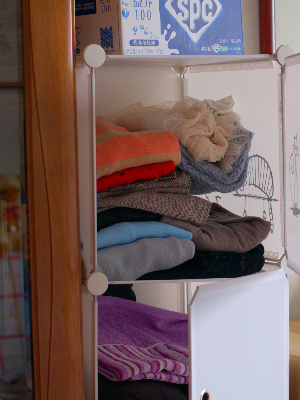
LOL Dataset. We first compare PyDiff with SOTA methods on the LOL dataset. The quantitative results are shown in Tab. 1. PyDiff outperforms other methods in all three metrics: PSNR, SSIM Wang et al. 2004, and LPIPS Zhang et al. 2018. Beating second place by 2.1 points on PSNR shows that PyDiff can recover more accurate colors. Surpassing second place by 1 point on SSIM shows that PyDiff accurately preserves more high-frequency details. Exceeding second place by 1 point on LPIPS shows that PyDiff gives more eye-pleasing results. Fig. 6 shows qualitative comparisons with other methods, where PyDiff exhibits the best result.
| Hyperparameters | Metrics | |||||
| PSNR | SSIM | LPIPS | FPS | |||
| LLFLOW | - | - | ||||
| PyDiff | ||||||
| 22.17 | 0.881 | 0.22 | ||||
| 3.81 | ||||||
| 4.97 | ||||||
| 5.86 | ||||||
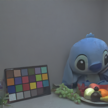
LOLV2 REAL PART. Since the test set of LOLV2 REAL PART overlaps with the training set of the LOL dataset, we combine the training set and test set of LOLV2 REAL PART and filter out the overlapping parts with the LOL training set by the ID of the images. For the filtered images, we sort them by ID and select 100 (i.e., the same size as the original test set) images with the smallest ID as the test set of LOLV2 REAL PART. Many of the selected images were taken at ISOs not included in the LOL training set, which is a good test of the model’s ability to deal with unseen noise. Tab. 2 shows the quantitative comparison with other SOTA methods on LOLV2 REAL PART. As PyDiff can deal with unseen noise better, it outperforms second place by 10.9 points on SSIM and 21 points on LPIPS. As shown in the second row of Fig. 7, other SOTA methods give results with significant noise, while PyDiff can remove noise well. At the same time, the first row of Fig. 7 also shows that PyDiff can better restore images with different exposure times.
LOLV2 SYNC PART. LOLV2 SYNC PART contains many illumination distributions that the LOL dataset does not have, and the scenarios in it are entirely different from the LOL dataset, which can test models’ generalization. Tab. 3 shows the quantitative comparison between PyDiff and other SOTA methods on LOLV2 SYNC PART. PyDiff shows competitive results and achieves first place in performance (e.g., 1.8 points higher than second place on SSIM), which demonstrates the generalization of PyDiff. Supplementary materials will show the qualitative comparison with other SOTA methods on LOLV2 SYNC PART.
5.3 Ablation Study
In this section, we conduct ablation studies on the main components of PyDiff to observe their impact on performance. The score for this section is calculated by combining the performance on the LOL dataset, LOLV2 REAL PART, and LOLV2 SYNC PART, which gives a better indication of the effectiveness of a component. FPS is measured on the LOL dataset (i.e., the resolution is ).
Downsampling Schedules. In Tab. 4, schedule represents vanilla diffusion models, which sample at a constant resolution. Our default setting, schedule , performs noisy sampling at a 1/2 resolution. Schedule is faster while slightly outperforming the schedule . Furthermore, our investigation revealed that faster schedules (e.g., , , and ) produce comparable results to the vanilla schedule . These findings indicate that noisier sampling can be performed at a lower resolution, while still maintaining high performance.
Position Encoding. Tab. 4 shows that the position encoding boosts PSNR and SSIM for PyDiff, which may tell networks about the change of resolution.
| Hyperparameters | Metrics | ||||
|---|---|---|---|---|---|
| PSNR | SSIM | LPIPS | FPS | ||
| (default) | |||||
Effectiveness of Global Corrector. Tab. 5 shows that the global corrector can bring improvements to PyDiff under various settings. Fig. 2 and Fig. 5(a)(c) show that the global corrector effectively alleviates global degradation. Furthermore, we can see from Tab. 5 that the global corrector gives little additional computational consumption to PyDiff.
Robustness to Batch Size. Tab. 5 shows that vanilla diffusion models without global corrector are very dependent on large batch size, which shows a significant performance drop when the batch size decreases. As our analysis in section 4.3, we argue that this is caused by the amplification factor, which has rigorous requirements for denoising networks. This problem has been significantly improved by adding a global corrector. As shown in Tab. 5, the global corrector enhances the performance of diffusion models under and outperforms the ones without global corrector under , which means that the global corrector can make diffusion models more robust to batch size and easier to train.
Comparison with LLFLOW. LLFLOW Wang et al. 2022 used to be first place on the LOL dataset based on the normalizing flow Dinh et al. 2016; Kingma and Dhariwal 2018. Both FLOWs and diffusion models are generative models that require multiple iterations. Therefore, it will be interesting to compare the speed of LLFLOW and PyDiff. According to Tab. 4, PyDiff significantly enhances performance, achieving an 87 faster speed than LLFLOW.
6 Conclusion
This paper proposes PyDiff, a diffusion model based method for low-light image enhancement. PyDiff uses a novel pyramid diffusion method, which makes sampling faster than vanilla diffusion models without any performance degradation. Furthermore, PyDiff uses a global corrector to alleviate global degradations that cannot be noticed by the denoising network and significantly improves performance with little additional computational consumption. Experimentally, PyDiff shows superior effectiveness, efficiency, and generalization ability on popular benchmarks. We hope that PyDiff will serve as a strong baseline for low-light image enhancement and that the pyramid diffusion method will facilitate the application of diffusion models in more low-level vision tasks.
Acknowledgement. This work is partially supported by the Fundamental Research Funds for the Central Universities (No. 226-2022-00051).
References
- Bao et al. [2022] Fan Bao, Chongxuan Li, Jun Zhu, and Bo Zhang. Analytic-dpm: an analytic estimate of the optimal reverse variance in diffusion probabilistic models. arXiv preprint arXiv:2201.06503, 2022.
- Chen et al. [2018] Chen Chen, Qifeng Chen, Jia Xu, and Vladlen Koltun. Learning to see in the dark. In Proceedings of the IEEE conference on computer vision and pattern recognition, pages 3291–3300, 2018.
- Choi et al. [2021] Jooyoung Choi, Sungwon Kim, Yonghyun Jeong, Youngjune Gwon, and Sungroh Yoon. Ilvr: Conditioning method for denoising diffusion probabilistic models. In 2021 IEEE/CVF International Conference on Computer Vision (ICCV), pages 14347–14356. IEEE, 2021.
- Cui et al. [2022] Ziteng Cui, Kunchang Li, Lin Gu, Shenghan Su, Peng Gao, Zhengkai Jiang, Yu Qiao, and Tatsuya Harada. Illumination adaptive transformer. arXiv preprint arXiv:2205.14871, 2022.
- Dhariwal and Nichol [2021] Prafulla Dhariwal and Alexander Nichol. Diffusion models beat gans on image synthesis. Advances in Neural Information Processing Systems, 34:8780–8794, 2021.
- Dinh et al. [2016] Laurent Dinh, Jascha Sohl-Dickstein, and Samy Bengio. Density estimation using real nvp. arXiv preprint arXiv:1605.08803, 2016.
- Fan et al. [2022a] Chi-Mao Fan, Tsung-Jung Liu, and Kuan-Hsien Liu. Half wavelet attention on m-net+ for low-light image enhancement. arXiv preprint arXiv:2203.01296, 2022.
- Fan et al. [2022b] Wan-Cyuan Fan, Yen-Chun Chen, DongDong Chen, Yu Cheng, Lu Yuan, and Yu-Chiang Frank Wang. Frido: Feature pyramid diffusion for complex scene image synthesis. arXiv preprint arXiv:2208.13753, 2022.
- Guo and Hu [2022] Xiaojie Guo and Qiming Hu. Low-light image enhancement via breaking down the darkness. International Journal of Computer Vision, pages 1–19, 2022.
- Guo et al. [2020] Chunle Guo, Chongyi Li, Jichang Guo, Chen Change Loy, Junhui Hou, Sam Kwong, and Runmin Cong. Zero-reference deep curve estimation for low-light image enhancement. In Proceedings of the IEEE/CVF Conference on Computer Vision and Pattern Recognition, pages 1780–1789, 2020.
- He et al. [2020] Jingwen He, Yihao Liu, Yu Qiao, and Chao Dong. Conditional sequential modulation for efficient global image retouching. In European Conference on Computer Vision, pages 679–695. Springer, 2020.
- Ho et al. [2020] Jonathan Ho, Ajay Jain, and Pieter Abbeel. Denoising diffusion probabilistic models. Advances in Neural Information Processing Systems, 33:6840–6851, 2020.
- Ho et al. [2022] Jonathan Ho, Chitwan Saharia, William Chan, David J Fleet, Mohammad Norouzi, and Tim Salimans. Cascaded diffusion models for high fidelity image generation. J. Mach. Learn. Res., 23:47–1, 2022.
- Jiang et al. [2021] Yifan Jiang, Xinyu Gong, Ding Liu, Yu Cheng, Chen Fang, Xiaohui Shen, Jianchao Yang, Pan Zhou, and Zhangyang Wang. Enlightengan: Deep light enhancement without paired supervision. IEEE Transactions on Image Processing, 30:2340–2349, 2021.
- Jin et al. [2022] Yeying Jin, Wenhan Yang, and Robby T Tan. Unsupervised night image enhancement: When layer decomposition meets light-effects suppression. In European Conference on Computer Vision, pages 404–421. Springer, 2022.
- Kim et al. [2021] Hanul Kim, Su-Min Choi, Chang-Su Kim, and Yeong Jun Koh. Representative color transform for image enhancement. In Proceedings of the IEEE/CVF International Conference on Computer Vision, pages 4459–4468, 2021.
- Kingma and Dhariwal [2018] Durk P Kingma and Prafulla Dhariwal. Glow: Generative flow with invertible 1x1 convolutions. Advances in neural information processing systems, 31, 2018.
- Land [1977] Edwin H Land. The retinex theory of color vision. Scientific american, 237(6):108–129, 1977.
- Lore et al. [2017] Kin Gwn Lore, Adedotun Akintayo, and Soumik Sarkar. Llnet: A deep autoencoder approach to natural low-light image enhancement. Pattern Recognition, 61:650–662, 2017.
- Lu et al. [2022] Cheng Lu, Yuhao Zhou, Fan Bao, Jianfei Chen, Chongxuan Li, and Jun Zhu. Dpm-solver: A fast ode solver for diffusion probabilistic model sampling in around 10 steps. arXiv preprint arXiv:2206.00927, 2022.
- Nichol and Dhariwal [2021] Alexander Quinn Nichol and Prafulla Dhariwal. Improved denoising diffusion probabilistic models. In International Conference on Machine Learning, pages 8162–8171. PMLR, 2021.
- Rombach et al. [2022] Robin Rombach, Andreas Blattmann, Dominik Lorenz, Patrick Esser, and Björn Ommer. High-resolution image synthesis with latent diffusion models. In Proceedings of the IEEE/CVF Conference on Computer Vision and Pattern Recognition, pages 10684–10695, 2022.
- Saharia et al. [2022a] Chitwan Saharia, William Chan, Huiwen Chang, Chris Lee, Jonathan Ho, Tim Salimans, David Fleet, and Mohammad Norouzi. Palette: Image-to-image diffusion models. In ACM SIGGRAPH 2022 Conference Proceedings, pages 1–10, 2022.
- Saharia et al. [2022b] Chitwan Saharia, Jonathan Ho, William Chan, Tim Salimans, David J Fleet, and Mohammad Norouzi. Image super-resolution via iterative refinement. IEEE Transactions on Pattern Analysis and Machine Intelligence, 2022.
- Song et al. [2020a] Jiaming Song, Chenlin Meng, and Stefano Ermon. Denoising diffusion implicit models. In Proc. of ICLR, 2020.
- Song et al. [2020b] Yang Song, Jascha Sohl-Dickstein, Diederik P Kingma, Abhishek Kumar, Stefano Ermon, and Ben Poole. Score-based generative modeling through stochastic differential equations. In International Conference on Learning Representations, 2020.
- Wang et al. [2004] Zhou Wang, Alan C Bovik, Hamid R Sheikh, and Eero P Simoncelli. Image quality assessment: from error visibility to structural similarity. IEEE Transactions on Image Processing, 13(4):600–612, 2004.
- Wang et al. [2022] Yufei Wang, Renjie Wan, Wenhan Yang, Haoliang Li, Lap-Pui Chau, and Alex Kot. Low-light image enhancement with normalizing flow. In Proceedings of the AAAI Conference on Artificial Intelligence, volume 36, pages 2604–2612, 2022.
- Wei et al. [2018] Chen Wei, Wenjing Wang, Wenhan Yang, and Jiaying Liu. Deep retinex decomposition for low-light enhancement. arXiv preprint arXiv:1808.04560, 2018.
- Whang et al. [2022] Jay Whang, Mauricio Delbracio, Hossein Talebi, Chitwan Saharia, Alexandros G Dimakis, and Peyman Milanfar. Deblurring via stochastic refinement. In Proceedings of the IEEE/CVF Conference on Computer Vision and Pattern Recognition, pages 16293–16303, 2022.
- Yang et al. [2021] Wenhan Yang, Wenjing Wang, Haofeng Huang, Shiqi Wang, and Jiaying Liu. Sparse gradient regularized deep retinex network for robust low-light image enhancement. IEEE Transactions on Image Processing, 30:2072–2086, 2021.
- Zhang et al. [2018] Richard Zhang, Phillip Isola, Alexei A Efros, Eli Shechtman, and Oliver Wang. The unreasonable effectiveness of deep features as a perceptual metric. In Proceedings of the IEEE Conference on Computer Vision and Pattern Recognition, pages 586–595, 2018.
- Zhang et al. [2019] Yonghua Zhang, Jiawan Zhang, and Xiaojie Guo. Kindling the darkness: A practical low-light image enhancer. In Proceedings of the 27th ACM international conference on multimedia, pages 1632–1640, 2019.
- Zhang et al. [2021] Yonghua Zhang, Xiaojie Guo, Jiayi Ma, Wei Liu, and Jiawan Zhang. Beyond brightening low-light images. International Journal of Computer Vision, 129(4):1013–1037, 2021.