Angle-based formation stabilization and maneuvers in port-Hamiltonian form with bearing and velocity measurements

To introduce the basic concepts, we consider the triangular formation as in Fig. 1. Hence, for the link $k$ between the agent $1$ and the agent $2$, we have

where $q_{1},q_{2}\in\mathbb{R}^{2}$ denote the position of agents $1$ and $2$, respectively, and $z_{k}\in\mathbb{R}^{2}$ is the relative position associated with the link $k$.

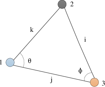
Regarding the constraints defining the formation geometric shapes, bearings and distances are simpler compared with angles. As shown in Fig. 1, bearings and distances are associated with two nodes and one edge while angles are associated with three nodes and two edges. Therefore, taking bearings and distances as an example, we give some definitions and conclusions. The distance and bearing between the agents $1$ and $2$ are given by

respectively. Moreover, we denote the general form of the constraints of the formation geometric shapes as $y_{k}\in\mathbb{Y}_{k}$, where $\mathbb{Y}_{k}$ is the constraint space. The time-evolution of $y_{k}$ is given by

where $L_{y_{k}}(z_{k})=\frac{\partial{y_{k}}}{\partial{z_{k}}}(z_{k})$ is the constraint Jacobian. Accordingly, for the bearing $s_{k}$ and the distance $r_{k}$, the corresponding Jacobians are given, respectively, by

where $I_{2}$ is the $2\times 2$ dimensional identity matrix. Henceforth, we omit the argument in the Jacobians $L_{s_{k}}$ and $L_{r_{k}}$ to simplify the notation.

Define $y_{k}^{*}$ as the desired value of the constraint $y_{k}$, corresponding to a desired formation. Then, we define the error

Hence, the control objective is to ensure that

To this end, we consider that the controller represents virtual couplings between the agents; see van2014port and duindam2009modeling. Specifically, virtual springs determine the formation shape, while virtual dampers inject damping, shaping the transient response. To illustrate this idea, we consider the link $k$ and the Hamiltonian (energy) function

where $c_{k}$ represents the constant stiffness matrix associated with the virtual springs. Note that the dimension of $c_{k}$ is determined by the constraint $y_{k}$. Hence, we propose the following dynamical system

where the velocity of the constraint $\omega_{k}\in T_{y_{k}}\mathbb{Y}_{k}$—with $T_{y_{k}}\mathbb{Y}_{k}$ the tangent space of $\mathbb{Y}_{k}$—can be understood as the input of the controller system, while the output $\gamma_{k}$ corresponds to the force exerted by the virtual couplings. In particular, $\frac{\partial{H_{k}}}{\partial{\tilde{y}_{k}}}$ represents the forces due to the virtual springs, and $d_{k}\omega_{k}$ the forces due to the virtual dampers, where $d_{k}\geq 0$ correspond to a constant dissipation matrix.

Note that the dynamics of the virtual couplings are expressed in the constraint space. However, to implement the controller, they can be transformed to $\mathbb{R}^{2}$ by means of the constraint Jacobian, i.e.,

where $\epsilon_{k}$ is the virtual force in $\mathbb{R}^{2}$.

According to port-Hamiltonian theory, we define $<e|f>:=e^{T}f$ as the power of a port with an effort $e$ and a flow $f$. Regarding the controller (7), $\gamma_{k}$ is the effort, and $\dot{\tilde{y}}_{k}$ is the flow in the constraint space. Correspondingly, $\epsilon_{k}$ and $\dot{z}_{k}$ are the effort and flow in $\mathbb{R}^{2}$, respectively. Note that the power in different spaces is the same since energy is coordinate-free.

Consider a group of $N$ agents with the topology of information exchange between these agents described by a graph $\mathcal{G}(\mathcal{V}_{N},\mathcal{E}_{E})$. It consists of a node set $\mathcal{V}$, where $\mathcal{V}=\{n_{1},n_{2},...,n_{N}\}$, and an edge set $\mathcal{E}\subseteq\mathcal{V}\times\mathcal{V}$, where $\mathcal{E}=\{e_{1},e_{2},...,e_{E}\}$. The incidence matrix $B\in\mathbb{R}^{N\times E}$ describes the relationship between the nodes and the edges, and it takes the following form:

In our work, we consider the particular class of strongly nondegenerate triangulated Laman graphs introduced in chen2017global. Moreover, we consider that the interaction topology is determined only by angles. A triangulated Laman graph is constructed from a line graph with two nodes; then, every newly added node is connected by two existing nodes which are also connected. An example is shown in Fig. 2 with $M$ triangles. The formation shape is determined by the marked angles. Note that assuming the underlying graph as a triangulated Laman graph is not restrictive. Any angle-based formation shape can be designed as a triangulated Laman graph with a new set of angle constraints.

Note that the graph considered here is undirected and the angle rigidity is ensured by Lemma 1 in jing2019angle, which is repeated below for the sake of completeness.

A framework is composed of a graph $\mathcal{G}_{N}$ and a realization which are positions of a group of agents, $q$. Angle rigidity means that the formation geometric shape is uniquely determined by a set of angles up to translations, scaling, and rotations by inner angles. For more details, see chen2020angle and jing2019angle.

We consider that the dynamics of the agents are given by double integrators with damping terms in $\mathbb{R}^{2}$, which are expressed in pH form as

where $q_{n}=(q_{x_{n}},q_{y_{n}})^{T}\in\mathbb{R}^{2}$, $n\in\{1,2,3\}$ denotes the position of the agent $n$, $p_{n}=(p_{x_{n}},p_{y_{n}})^{T}=(m_{n}\dot{q}_{x_{n}},m_{n}\dot{q}_{y_{n}})^{T}\in\mathbb{R}^{2}$ denotes the momentum, and $m_{n}$ denotes the mass. Moreover, $U_{n}=(U_{x_{n}},U_{y_{n}})^{T}\in\mathbb{R}^{2}$ and $Y_{n}=(Y_{x_{n}},Y_{y_{n}})^{T}\in\mathbb{R}^{2}$ denote the input and output, respectively, and $H_{n}(p_{n})$ is the Hamiltonian of the agent $n$.

We assume that each agent has access to bearing and relative velocity information. For relative velocity information, each agent is either able to measure and communicate its own velocity or measure the relative velocity directly. In addition, we assume that the communication topology is connected in each triangle, therefore, the agent has access to the bearing measurement of the non-adjacent edge. For example, as shown in Fig. 1, agent $1$ has access to the bearing measurement $s_{i}$. Since the constraints of the formation geometric shape are given by angles and agents can measure the bearings of their neighboring agents, we use the cosine function of the angle to represent the value of the angle, which can be easily calculated by bearing measurements. Hence, for the angle $\theta$, the definition is given by

The objective of this paper is to design a controller using only bearing and velocity measurements that ensures the group of agents with an underlying triangulated Laman graph, modeled by (9) to achieve a desired formation constrained by angles, while simultaneously achieving velocity tracking, and scale and orientation control.

We first consider the controller of agent $1$. Since the movement of agent $1$ affects both $\theta$ and $\phi$, the controller of agent $1$ consists of two parts. One is to satisfy the constraint on $\theta$, and the other satisfies the constraint on $\phi$.

For $\theta$, we use the cosine function to represent the angle measurement. Given (10), the control aim is to design a controller to ensure that $s_{k}^{T}s_{j}$ converge to the desired value $({s_{k}^{T}s_{j}})^{*}$. Hence, we define the error

In order to guarantee that the system converges to the desired state, i.e., the error (15) converges to zero, it is necessary to assign a potential energy of the angle to the closed-loop system. To this end, we propose the following Hamiltonian function

where $c_{\theta 1}\in\mathbb{R}_{+}$ is a constant.

The corresponding port-Hamiltonian controller composed of a spring and a damper is given as

where $\omega_{\theta 1}$ denotes the input of the controller, and $d_{\theta 1}\in\mathbb{R}_{+}$ is the corresponding damping parameter. Here, $\gamma_{\theta 1}$ is the resulting virtual force in the space of angle constraint. Furthermore, the power of the port is given as

where $\dot{\widetilde{(s_{k}^{T}s_{j})}}$ is the flow and $\gamma_{\theta 1}$ is the effort. Here we only consider a part of the time derivative of the angle $\theta$ caused by the movement of agent $1$. To transform the power from the angle space to $\mathbb{R}^{2}$, we compute

The effort of the port in (19) relies on the distance information which is not measurable. In order to avoid distance measurement, we use the relative velocity measurement to estimate the unknown distance.

Note that since we assume that the distance is estimated rather than measured, the distance term in the angle Jacobian needs to be replaced accordingly. As a result, the estimated angle Jacobian is given by

where $\hat{r}_{\theta k}$ is the distance estimate of the edge $k$ for the control of angle $\theta$, and $\hat{r}_{\theta j}$ is the distance estimate of edge $j$ for the control of angle $\theta$. Correspondingly, $\hat{L}_{\theta s_{k}},\hat{L}_{\theta s_{j}}$ are the estimated bearing Jacobian of $s_{k}$ and $s_{j}$, respectively, for the control of angle $\theta$.

However if $\hat{L}_{\theta 1}$ is used to replace $L_{\theta 1}$ in the right side of (19), the equation is not satisfied because the effort $\gamma_{\theta 1}$ corresponds to the real flow $\frac{{\rm d}(s_{k}^{T}s_{j})}{{\rm d}t}$ in the angle space. It causes the discrepancy of the power through the virtual coupling due to the error between the estimated distance and the real unknown distance. To handle the discrepancies, we define the distance errors as $\bar{r}_{\theta k}:=\hat{r}_{\theta k}-r_{k}$, and $\bar{r}_{\theta j}:=\hat{r}_{\theta j}-r_{j}$. To calculate the estimated effort in $\mathbb{R}^{2}$, we have

where $\alpha_{\theta k}=\frac{r_{k}}{\hat{r}_{\theta k}}\gamma_{\theta 1}$ is the estimated effort related to $\hat{r}_{\theta k}$ and $\alpha_{\theta j}=\frac{r_{j}}{\hat{r}_{\theta j}}\gamma_{\theta 1}$ is the estimated effort related to $\hat{r}_{\theta j}$.

Furthermore, considering the ports in different spaces, we have that

Comparing (19) with (22), the discrepancy between the real effort and the estimated effort can be derived as

The power of ports with $\beta_{\theta k}$, $\beta_{\theta j}$ as the efforts are given by

To account for the power associated with the ports in distance space, we define the corresponding Hamiltonians as

where $c_{\theta k},c_{\theta j}\in\mathbb{R}_{+}$ are constants.

The power of the ports in distance space is given by

Since the energy is coordinate-free, the power in angle space and distance space are the same. Therefore, comparing (24) and (26), we have

Similarly,

Furthermore, the dynamics of the estimators are given by

Similarly,

Note that we only use the information of relative velocity and bearing measurement in the above estimators, while distance measurement is not used.

The resulting control law of agent $1$ for angle $\theta$ is given by feedback connection of the original system and the effort in $\mathbb{R}^{2}$ with the estimated distance, which can be summarized by substituting (17) and (20) into (21) and adding a negative sign as

In this section, we design the controller of agent $1$ for the control of angle $\phi$. Define the Hamiltonian

where $c_{\phi 1}\in\mathbb{R}_{+}$ is a constant. The controller with spring and damping terms are given by

where $\omega_{\phi 1}$ denotes the input of the controller. $d_{\phi 1}\in\mathbb{R}_{+}$ is the corresponding damping parameter.

Considering the ports in different spaces, we have that

where $\hat{L}_{\phi 1}$ is the estimated angle Jacobian mapping from the position of the agent $1$ to the angle $\phi$ and $\hat{L}_{\phi s_{k}}$ is the estimated bearing Jacobian of $s_{k}$ for the control of angle $\phi$. Furthermore, $\hat{r}_{\phi k}$ is the estimated distance of the edge $k$ for the control of angle $\phi$.

Taking the same steps as in Section 3.1 leads to the following estimator

where $c_{\phi k}\in\mathbb{R}_{+}$ is a constant.

Correspondingly, the control law of the agent $1$ for the angle $\phi$ is given by

To sum up, the control law of the agent $1$ is given by

The controller design for the agents $2$ and $3$ is similar to the agent $1$, so we omit some details for the following analysis.

For the agent $2$, there are two parts in the control law. The first part is to control the angle $\theta$, whose corresponding Hamiltonian and controller in the angle space are given by

where $\omega_{\theta 2}$ denotes the input of the controller. $c_{\theta 2},d_{\theta 2}\in\mathbb{R}_{+}$ are constants. The corresponding estimated angle Jacobian and distance estimators are given by

The second part is to control the angle $\phi$, whose corresponding Hamiltonian and controller are given by

where $\omega_{\phi 2}$ denotes the input of the controller, and $c_{\phi 2},d_{\phi 2}\in\mathbb{R}_{+}$ are constants. The corresponding estimated angle Jacobian and distance estimators are given by

Note that the expressions (35) and (45) are both distance estimators of the edge $k$, but (35) is estimated by the agent $1$, while (45) is estimated by the agent $2$.

The power from the port related to agent $2$ is given by

Correspondingly, the control law of the agent $2$ is given by

For the agent $3$, there are also two parts in the control law. The first part is to control the angle $\phi$, whose corresponding Hamiltonian and controller in angle space are given by

where $\omega_{\phi 3}$ denotes the input of the controller, and $c_{\phi 3},d_{\phi 3}\in\mathbb{R}_{+}$ are constants. The corresponding estimated angle Jacobian and distance estimators are given

where $c_{\phi i},c_{\phi j}\in\mathbb{R}_{+}$ are constants.

The second part is to control the angle $\theta$. The corresponding Hamiltonian and controller in angle space are given by

where $\omega_{\theta 3}$ denotes the input of the controller, and $c_{\theta 3},d_{\theta 3}\in\mathbb{R}_{+}$ are constants. The corresponding estimated angle Jacobian and distance estimators are given by

where $c_{\theta i}\in\mathbb{R}_{+}$ is a constant. Note that the expressions (41) and (56) are both distance estimators of the edge $i$, but (41) is estimated by the agent $2$, while (56) is estimated by the agent $3$.

The power from the port related to agent $3$ is given by

References

- [1] Randal W. Beard, Jonathan Lawton, and Fred Y. Hadaegh. A coordination architecture for spacecraft formation control. IEEE Transactions on control systems technology, 9(6):777–790, 2001.
- [2] Wei Ren, Randal W. Beard, and Ella M. Atkins. Information consensus in multivehicle cooperative control. IEEE Control systems magazine, 27(2):71–82, 2007.
- [3] Kwang Kyo Oh, Myoung Chul Park, and Hyo Sung Ahn. A survey of multi-agent formation control. Automatica, 53:424–440, 2015.
- [4] Jorge Cortés and Magnus Egerstedt. Coordinated control of multi-robot systems: A survey. SICE Journal of Control, Measurement, and System Integration, 10(6):495–503, 2017.
- [5] Yuanchang Liu and Richard Bucknall. A survey of formation control and motion planning of multiple unmanned vehicles. Robotica, 36(7):1019–1047, 2018.
- [6] Fei Chen and Wei Ren. On the control of multi-agent systems: A survey. Foundations and Trends® in Systems and Control, 6(4):339–499, 2019.
- [7] Emmanuel Nuno, Antonio Loria, Tonatiuh Hernandez, Mohamed Maghenem, and Elena Panteley. Distributed consensus-formation of force-controlled nonholonomic robots with time-varying delays. Automatica, 120:109114, 2020.
- [8] Meng Ji and Magnus Egerstedt. Distributed coordination control of multiagent systems while preserving connectedness. IEEE Transactions on Robotics, 23(4):693–703, 2007.
- [9] Brian D. O. Anderson, Changbin Yu, Baris Fidan, and Julien M. Hendrickx. Rigid graph control architectures for autonomous formations. IEEE Control Systems Magazine, 28(6):48–63, 2008.
- [10] Ming Cao, Changbin Yu, and Brian D. O. Anderson. Formation control using range-only measurements. Automatica, 47(4):776–781, 2011.
- [11] Shiyu Zhao, Zhenhong Li, and Zhengtao Ding. Bearing-only formation tracking control of multiagent systems. IEEE Transactions on Automatic Control, 64(11):4541–4554, 2019.
- [12] Minh Hoang Trinh, Shiyu Zhao, Zhiyong Sun, Daniel Zelazo, Brian D. O. Anderson, and Hyo Sung Ahn. Bearing-based formation control of a group of agents with leader-first follower structure. IEEE Transactions on Automatic Control, 64(2):598–613, 2018.
- [13] Gangshan Jing, Guofeng Zhang, Heung Wing Joseph Lee, and Long Wang. Angle-based shape determination theory of planar graphs with application to formation stabilization. Automatica, 105:117–129, 2019.
- [14] Liangming Chen, Ming Cao, and Chuanjiang Li. Angle rigidity and its usage to stabilize multi-agent formations in 2d. IEEE Transactions on Automatic Control, 2020.
- [15] Ningbo Li, Pablo Borja, Arjan van der Schaft, Jacquelien MA Scherpen, and Liangming Chen. Angle formation of double integrator with bearing and velocity information. IFAC-PapersOnLine, 54(19):217–222, 2021.
- [16] Ewoud Vos, Jacquelien Scherpen, Arjan van der Schaft, and Ate Postma. Formation control of wheeled robots in the port-hamiltonian framework. IFAC Proceedings Volumes, 47(3):6662–6667, 2014.
- [17] Geoff Stacey and Robert Mahony. A passivity-based approach to formation control using partial measurements of relative position. IEEE Transactions on Automatic Control, 61(2):538–543, 2015.
- [18] Ming Xu and Yuying Liang. Formation flying on elliptic orbits by hamiltonian structure-preserving control. Journal of Guidance, Control, and Dynamics, 41(1):294–300, 2018.
- [19] Ningbo Li, Jacquelien Scherpen, Arjan Van der Schaft, and Zhiyong Sun. A passivity approach in port-hamiltonian form for formation control and velocity tracking. In 2022 European Control Conference (ECC), pages 1844–1849. IEEE, 2022.
- [20] Arjan J Van der Schaft. L2-gain and passivity techniques in nonlinear control, volume 2. Springer, 2000.
- [21] Hassan K Khalil. Nonlinear Systems. Third Edition, Prentice Hall, New Jersy, 2002.
- [22] Arjan J van der Schaft and B. M. Maschke. Port-Hamiltonian systems on graphs. SIAM Journal on Control and Optimization, 51(2):906–937, 2013.
- [23] Robert Mahony and Stefano Stramigioli. A port-hamiltonian approach to image-based visual servo control for dynamic systems. The International Journal of Robotics Research, 31(11):1303–1319, 2012.
- [24] Meysam Basiri, Adrian N. Bishop, and Patric Jensfelt. Distributed control of triangular formations with angle-only constraints. Systems & Control Letters, 59(2):147–154, 2010.
- [25] Liangming Chen and Zhiyong Sun. Globally stabilizing triangularly angle rigid formations. IEEE Transactions on Automatic Control, 2022.
- [26] Liangming Chen, Hector Garcia de Marina, and Ming Cao. Maneuvering formations of mobile agents using designed mismatched angles. IEEE Transactions on Automatic Control, 67(4):1655–1668, 2021.
- [27] Arjan J van der Schaft and Dimitri Jeltsema. Port-Hamiltonian systems theory: An introductory overview. Foundations and Trends® in Systems and Control, 1(2-3):173–378, 2014.
- [28] Vincent Duindam, Alessandro Macchelli, Stefano Stramigioli, and Herman Bruyninckx. Modeling and control of complex physical systems: the port-Hamiltonian approach. Springer Science & Business Media, 2009.
- [29] Xudong Chen, Mohamed Ali Belabbas, and Tamer Basar. Global stabilization of triangulated formations. SIAM Journal on Control and Optimization, 55(1):172–199, 2017.