Master’s Thesis (Academic Year 2022)
RuLa: A Programming Language for RuleSet-based Quantum Repeaters
A thesis presented for the degree of
Master of Media and Governance
Keio University
Graduate School of Media and Governance
Ryosuke Satoh
Abstract of Master’s Thesis Academic Year 2022
RuLa: A Programming Language for RuleSet-based Quantum Repeaters
Quantum Repeaters are one critical technology for scalable quantum networking. One of the key challenges regarding quantum repeaters is their management of how they provide quantum entanglement for distant quantum computers. We focus on the RuleSet architecture, which is a decentralized way to manage repeaters. The RuleSet concept is designed to scale up the management of quantum repeaters for future quantum repeaters, suitable because of its flexibility and asynchronous operation, however, it is still at the conceptual level of definition and it is very hard to define raw RuleSets. In this thesis, we introduce a new programming language, called “RuLa”, to write the RuleSets in an intuitive and coherent way. The way RuLa defines RuleSet and Rule is very similar to how the Rule and RuleSets are executed, so that the programmer can construct the RuleSets the way they want repeaters to execute them. We provide some examples of how the RuleSets are defined in RuLa and what is the output of the compilation. We also discussed future use cases and applications of this language.
Keywords: 1. Quantum Networking, 2. Quantum Repeater, 3.RuleSet,
4. Domain Specific Language,
Keio University
Graduate School of Media and Governance
Ryosuke Satoh
Contents
List of Figures
List of Tables
Chapter 1 Introduction
1.1 Background
Quantum technology has been one of the biggest technological challenges in recent decades. Quantum computers have been built and are even available to researchers and students around the world through the cloud system [1]. Recently, Google claimed quantum supremacy, which demonstrated that quantum computers experimentally exceed classical computers in terms of computational power [2] (In another paper, quantum computing simulation with more than fifty qubits [3] has been demonstrated). Quantum communication is also a very active research field that has also gained research interest over the years because of its uniqueness and a wide variety of applications.
Quantum communication allows us to connect multiple quantum computers or small quantum processors to exchange quantum states using quantum teleporation [4], enhance quantum computational power [5], and securely transfer classical information through a public quantum channel using quantum key distribution [6]. In addition to these, we can use quantum communication to improve the sensitivity of sensor networks [7].
However, there is a huge gap between the current status of quantum networking development and the quantum networks that are capable of running those applications. Current state-of-the-art experiments have shown entanglement generation in a few hops of quantum devices [8, 9]. The biggest challenge is to keep the entangled qubits in a nearly perfect state for a long time. Researchers have put a great deal of effort into hardware development to improve the coherence time of quantum memories [10, 11], to reduce the errors and losses in fiber.
In addition to the quality of the hardware, the architecture and protocols of quantum networks are also important to develop truly useful quantum networks [12, 13]. RuleSet protocol [14, 13] is one of the research projects that define how to manage quantum repeaters, which is one of the most important components in quantum networking. This approach supports scalable asynchronous operations for quantum repeaters, and it is easy to distribute the generated RuleSet to intermediate quantum repeaters. However, one of the biggest difficulties is creating a large number of RuleSets, especially when there are complex Rules inside the RuleSet.
In this thesis, we approach this problem by making a new programming language to define the RuleSet and the corresponding systems to generate a large number of RuleSets.
1.2 Research Contribution
The main research contribution of this project is to develop a new programming language called RuLa that makes it easier to write and execute RuleSets.
The key idea for scalable RuleSet generation is to provide an abstract way to define multiple rules with flexible configurations. In addition, since RuleSet does not allow any condition operators such as if~else, Rula introduces a higher-level condition that is automatically translated into several different condition clauses in different rules. RuLa provides a way to modularly define the Rules that allows us to improve the visibility and maintainability of the RuleSet.
We assume two types of users who would find this project beneficial. One is for users who want to try a new quantum networking protocol in the formulation of the RuleSet. Since RuleSet is fairly general for describing any operation in quantum networking, it is possible to implement a new protocol in a RuleSet format. RuLa allows this user to accelerate the development cycle by providing a user interface to generate RuleSets.
The second user is the network manager who actually manages the quantum network in the future. This could be a human manager who decides how the repeaters work or even a computer program that automatically deals with requests from other quantum computers. Once the way of generation of the RuleSet is defined in RuLa, it is possible to generate an arbitrary number of RuleSets by only changing its configurations.
1.3 Thesis Structure
This thesis is structured as follows. Chapter 2 provides basic preliminary knowledge on quantum information processing, such as the mathematical representation of qubits, quantum circuits, and entanglement. It also introduces the current status of quantum networking development and important protocols for quantum communications. The problems to be tackled in this thesis are defined in Chapter 3. The actual contents of RuleSet and how the RuleSet is described are also explained in this chapter. In Chapter 4, actual proposals including language design decisions and how the compiler works are explained with its requirements and assumptions. Finally, we evaluate our proposals in terms of their feasibility, use cases, and scalability in Chapter 5 and conclude this thesis in Chapter 6.
Chapter 2 Preliminaries
This chapter covers preliminary knowledge of quantum computing and networking from an overview of the history of quantum information processing and fundamental calculation to specific types of operation such as entanglement swapping and purification, which are very important protocols in quantum communications. In addition to that, this chapter introduces the concept of domain-specific languages.
2.1 History of Quantum Technology
Quantum technology in the 21st century is more than just a theory in research papers. Real quantum computers and networks have been deployed and operated by companies, universities, and national labs. Researchers in several fields in academia, leading companies, and startups are getting involved in this world competition for developing large quantum computers and networks to see the next generation of computation.
The term “quantum computer” was proposed by Richard Feynman in a talk at a conference in 1981 [15]. His original motivation for building a quantum computer was to simulate quantum systems. In general, simulating a large quantum system is a very hard task for our laptop computers, and he thought it was more natural to simulate such a complex system with quantum computers.
As Feynman proposed, simulating a quantum system is a promising application of quantum computing [16]. Quantum computing allows us to simulate complex quantum systems more precisely and faster. Researchers demonstrated the calculation of the energy surface of molecular hydrogen in 2016 with a real superconducting quantum device [17, 18].
A qubit is the heart of a quantum computer that can be implemented by different types of physical systems. One of the prominent examples is the superconducting qubit proposed by Nakamura et al. in [19]. There are also qubits with photons [20, 21] and trapped ions [22].
Current quantum computers that are called NISQ (Noisy Intermediate Scale Quantum) devices do not have error correction capability and do not scale up for more complex problems and algorithms [23]. However, computational power is reaching the edge of what classical computers cannot do. In 2019, Google claimed that its quantum processor ”Sycamore” experimentally outperformed classical computers and achieved quantum supremacy [2] (However, the result has been still controversial because the simulation of more than fifty qubits was also demonstrated [3]). Quantum computational advantage has also been demonstrated by using photonic quantum computers with solving gaussian boson sampling on top of their quantum computers [24].
In quantum communication, the first loophole-free CHSH experiment has been demonstrated, which shows the feasibility of generating genuine entangled states over a distance [25]. There is also a demonstration of Quantum Key Distribution (QKD) with satelite [26]. This experiment shows that it is possible to actually apply QKD protocols over the globe.
2.2 Qubit
The qubit is a quantum analogue of tge bit in classical computers and is a fundamental unit of quantum information processing. Unlike a classical bit representing ’0’ or ’1’ deterministically, a qubit could be a superposition of ’0’ and ’1’.
2.2.1 Notation
Dirac’s bra-ket notation invented by Paul Dirac [27] is a powerful representation of the quantum state. A quantum state can be represented by a vector in a Hilbert space . As the simplest example, the zero (one) state can be represented as ().
| (2.2.1) |
The superposition of the quantum states can be represented as linear combinations of the computational basis states.
| (2.2.2) |
where and are complex coefficients () that satisfy the relationship . For example, when , , the quantum state is
| (2.2.3) |
which is an equal superposition of the basis states and (, ).
If there are bases in a state, the superposition of all basis states is as follows.
| (2.2.4) |
The sum of the squared coefficients must also be 1 ().
It is simply possible to extend this representation to the multi-qubit quantum state. The multi-qubit quantum state can be constructed by tensor products of qubit states.
| (2.2.5) |
The resulting Hilbert space is just a tensor product of two Hilbert spaces (). When there are qubits in the system and all the qubit states are , the quantum state is
| (2.2.6) |
An qubit state can be represented as a vector with elements.
We can also simply represent the inner product and the outer product of quantum states with the bra-ket notation. Let and be quantum states and where and are complex probability amplitudes (). The inner product of two quantum states is
| (2.2.7) |
Their outer product is
| (2.2.8) |
The density matrix is one good way to represent a mixed state to introduce noise into a quantum state. If a qubit is in pure state , the density matrix of is
| (2.2.9) |
When the target quantum state is noisy, we probably have unwanted quantum states in some probability.
| (2.2.10) |
In the simplest example, if a qubit state flips with 20 chance, the density matrix is as follows:
| (2.2.11) | ||||
| (2.2.12) | ||||
| (2.2.13) |
where () is the density matrix of pure state ().
2.2.2 Bloch Sphere
A Bloch sphere shown in Figure 2.1 is a representation of one qubit state. A vector inside the Bloch sphere represents the current quantum state, and the north pole represents the state. The surface of the Bloch sphere is the of possible quantum states that one pure qubit can have.
The points of each axis correspond to the following quantum states.
where the superscript represents the positive (negative) directions in the Bloch sphere.
2.2.3 Implementation
Superconducting qubits are one promising candidate for physical qubits (e.g. They come in several types from Cooper-pair box [19], Transmon [29]), which many companies pursue due to its possibility of fault-tolerant quantum computing. Trapped ions [30] and linear optical qubits [31] are also said to be good candidates for scalable quantum computing.
However, any quantum system that satisfies DiVincenzo’s criteria proposed in [32] can be a candidate for a qubit. There are five criteria for the quantum computing qubit and two criteria for the quantum communication qubit. A qubit needs to have the following characteristics.
- 1.
Scalable physical system with well-characterized qubit
- 2.
Capability of initialization to fiducial state
- 3.
Longer decoherence time than its gate operation time
- 4.
Capability of operating a universal set of gates
- 5.
Measurable a specific qubit
In addition to those, the qubits for quantum communication need to satisfy the following criteria.
- 6.
Capable of converting a flying qubit to a stationary qubit
- 7.
Transmittable a flying qubit between specified locations.
In terms of criteria 6 and 7, the trapped ion, the Nitrogen-vacancy center in diamond quantum memory [33] are good candidates for quantum communication. However, there is also research work that tries to communicate between superconducting qubits via photonic conversions [34].
2.3 Quantum Information Processing
A qubit as introduced in Section 2.2 is nothing more than an information unit that represents a quantum state. To compute some algorithms and calculations on top of it, we need to manipulate those qubits to interpret a problem. The physical controls for these qubits are different in different physical implementations. However, operations can be written as a form of a unitary matrix.
2.3.1 Quantum Gates
Quantum Circuit is one convenient representation of a set of quantum operations such as the one shown in Figure 2.2.
The horizontal lines represent qubits, and operations are performed from left to right. The boxes are the quantum gate that corresponds to some operation on a single qubit. There are also two-qubit gates which are represented as a combination of line and circle. The black dot is the control qubit and the other edge of the vertical line is the target qubit. At the end of the circuit, usually we measure the qubit represented, as a meter mark, and get some classical outputs.
2.3.2 Hadamard Gate
Hadamard gate is a fundamental quantum operation that creates the superposition of a single qubit.
Hadamard gate can be written in matrix form as
| (2.3.1) |
When the initial state is and the H gate is applied to it, the resulting state is,
| (2.3.2) | ||||
| (2.3.3) |
which is known as one of the equal superposition states in a single qubit state.
2.3.3 Pauli Gates
Pauli gates (X, Y, Z) are also important quantum operations that correspond to rotations about the corresponding axis of the Bloch sphere. The matrices of Pauli X, Y, and Z are
| (2.3.4) |
Those operations are the rotation over the corresponding bases. Pauli X gate flips to vice versa, and the Z gate applies phase rotation to . When the original state is , the Pauli Z operation gives us which introduces a global phase.
2.3.4 Controlled NOT (X) Gate
Controlled NOT gate, CNOT gate, in short, is a quantum operation over two different qubits.
Figure 2.4 shows the gate representation of the CNOT gate. When the first (top) qubit is , the CNOT gate applies the X gate to the second (bottom) qubit. For example, when the initial state is , the state becomes . CNOT gate is represented by a four-by-four matrix because it covers two qubits.
| (2.3.5) |
2.3.5 Controlled Z Gate
Controlled Z (CZ) gate is similar to the Controlled NOT gate, but the target operation is not the Pauli X gate, but the Pauli Z gate.
When the first qubit is , this gate applies the Z gate to the second qubit. The CNOT gate and the CZ gate are interchangeable since Pauli X and Z are interchangeable over the Hadamard gate.
2.3.6 Measurement
To extract information from the quantum state, we need to measure the qubit and observe it as a classical result. Let be a collection of measurement operators where is the corresponding computational basis state, and be the measured quantum state. The probability of observing a basis state is
| (2.3.6) |
For example, when we measure on the two computational bases and ,
| (2.3.7) | |||
| (2.3.8) |
The probability of measuring is 1 and is 0. However, when we measure on different bases, for example and ,
| (2.3.9) | |||
| (2.3.10) |
It is also possible to construct a measurement operation for more than a single qubit. One frequently used basis in quantum communication is the Bell measurement, which measures in a Bell basis (see details on the Bell state in Section 2.4.3).
2.3.7 Noise
When a qubit is placed in a completely closed and perfect system, its state could always be perfect, and that qubit always tells us the actual quantum state. However, the reality is different, and its state could be far from the ideal state. A quantum state can interact with the outer world and become a noisy quantum state.
There are multiple types of noisy channels in the quantum world.
Bit flip channel: One of the simplest types of errors is the bit flip error, which can also occur in classical bits. Suppose that the bit-flip error occurs with probability . The noisy quantum state can be described as
| (2.3.11) | ||||
| (2.3.12) |
where is the ideal state without noise.
Phase flip channel: Similar to the bit flip error, we can also think of the phase flip error by introducing Z errors in the quantum state.
| (2.3.13) |
Depolarizing channel: The depolarizing channel is an important error type in the quantum world, in which a qubit becomes a completely mixed state with some probability.
| (2.3.14) |
where is the identity matrix and is the dimension of the quantum system. More generally, satisfies the following equation for arbitrary .
| (2.3.15) |
where , and are Pauli matrices defined in Equation 2.3.4 Thus, Equation 2.3.14 can be rewritten as
| (2.3.16) |
2.3.8 Fidelity
Fidelity is a metric that measures the distance between two quantum states. The fidelity between two quantum states and is defined as
| (2.3.17) |
where tr is trace of the resulting matrix. It is also possible to measure the fidelity between the pure state and an arbitrary quantum state as
| (2.3.18) |
For example, if we measure the fidelity between and ,
| (2.3.19) |
The fidelity between and is,
| (2.3.20) |
where is the density matrix of a pure state .
2.4 Entanglement
Entanglement is a fundamental phenomenon in quantum systems that shows a stronger correlation between two quantum systems. This correlation cannot be mimicked by the classical correlation.
2.4.1 Bell State
A fundamental example of entangled states is given by the four Bell states, which can be
| (2.4.1) | ||||
| (2.4.2) | ||||
| (2.4.3) | ||||
| (2.4.4) |
The first and the second qubits are strongly correlated and the state cannot be determined separately when they are measured. For example, when the first qubit in 2.4.1 is , the second qubit is measured as respectively.
2.4.2 Multipartite Entangled State
It is also possible to think that more than two quantum bits are entangled. A particular example of a three-qubits entangled state is given by the GHZ (Greenberger-Horne-Zeilinger) state [35].
| (2.4.5) |
In general, an qubit GHZ state is
| (2.4.6) |
Another example of a multipartite entangled state is a graph state. Suppose that we have a graph that is composed of a set of vertices and edges . The qubits in a system are corresponding to the vertices of the target graph and the entanglement between two qubits are edges in the graph. The following equation shows how the graph state is created.
| (2.4.7) |
All the qubits are initialized into superposition state , and CZ gates are applied according to the edges of the target graph.
2.4.3 Bell Measurement
Let be the Bell state shown in Equation 2.4.1. If we measure this Bell state on the following Bell basis,
| (2.4.8) | ||||
| (2.4.9) |
The measurement result of can be written as follows.
| (2.4.10) | ||||
| (2.4.11) | ||||
| (2.4.12) | ||||
| (2.4.13) |
Measurement in the Bell basis is very important in quantum communication. It is used to perform the entanglement swapping explained in Section 2.7.
2.4.4 CHSH Experiment
In [36], John Stewart Bell stated the upper limit of correlations in hidden local variables. However, this Bell’s theorem was revealed to be not applicable to quantum physics. In [37], Bell explained the violation of his previous theorem. To prove the existence of the entanglement, the extended inequality called the CHSH inequality is supposed to be satisfied.
Suppose that there are two people, Alice and Bob, who select two numbers from either +1 or -1 at randomly without coordination. Let and be the values that Alice chose, and and be the values that Bob chose.
If we think of the following quantity,
| (2.4.14) |
where either or becomes 0 so that the possible values that 2.4.14 can take are . The following inequality holds when we consider the expectation values for each combination.
| (2.4.15) |
However, when it comes to the quantum system, Equation 2.4.15 no longer holds.
Alice and Bob prepare two measurement basis. Let and be the measurement basis of and . Bob chooses and as and which are diagonal to Alice’s basis.
If Alice and Bob share one of the Bell states , and measure it on the corresponding basis, the maximum expectation values of the measurement results are the following.
| (2.4.16) | ||||
| (2.4.17) |
where is the average observable value. Thus, the total expectation value is
| (2.4.18) |
The generation of entanglement has been demonstrated experimentally and [25] is the first demonstration without any loopholes.
2.5 Quantum Communication
Quantum computing has promising applications such as quantum simulation, factoring, data search in databases, and optimization. However, quantum communication allows us to scale up and think of more complex applications. Shor’s algorithm requires 20 million noisy qubits to factor in 2048-bit RSA as reported in [38]. Preparing such a large number of qubits is not realistic if we assume only the capacity of a single quantum processor. Quantum communication plays an important role here in making quantum computing scalable. The simplest case is to connect several quantum processors to each other by preparing a bus, as we do on our laptops. In [39], the authors proposed a method to achieve arithmetic on distributed quantum processors that might allow us to implement Shor’s algorithm in a distributed manner.
2.5.1 Quantum Networking Stack
There are proposed layering models for quantum communications that are modeled based on the roles in the network [12, 40, 41].

Figure 2.6 is a proposed layering model for quantum networking there are roughly four or five layers from the physical layer up to the application layer.
- •
Application: The layer responsible for managing end-to-end applications such as distributed quantum computing and quantum key distribution. The application layer consumes generated entanglement in the network layer.
- •
Network: The network layer is responsible for end-to-end entanglement generation and management to reach the requirements for the applications.
- •
Link: The link layer is in charge of generating entanglement with neighboring nodes for passing that link-level entanglement to the network layer. The link layer is also responsible for managing errors for link-level entanglement.
- •
Physical: This layer contains complex hardware and firmware that allow us to generate entanglement and manipulate the actual qubit to generate entanglement.
2.5.2 Applications
Many applications of quantum communication have been proposed, and a promising application is distributed quantum computing (DQC), which allows us to scale up the capability of quantum computing by connecting multiple quantum computers with quantum links [42, 43].
Quantum key distribution (QKD) is another very prominent example of a quantum networking application [44, 6]. In a shared key cryptosystem, one of the biggest challenges is sharing the generated key securely. Public key cryptography solved that problem by asymmetric key generation. One of the most famous asymmetric key generation protocols is Diffie–Hellman key exchange protocol which allows us to generate a secret key from a public key that is shared with anyone in the world. The point is that we do not have to expose the generated secret key in public to share it. The security of this protocol is supported by the complexity of the modular exponentiations. After the Diffie-Hellman key exchange was proposed, RSA cryptography was proposed [45] that allows us to authenticate and sign digital signatures. However, as Peter Shor revealed in [46], the problem of prime number factoring on which RSA relies for its security became known as a polynomial-time solvable problem using quantum computers. Most of the current cryptosystem relies on RSA or a discrete logarithmic problem, and those are said to be solved by quantum computers, so we have to invent a new method to share our information securely. One way to do this is to develop a completely new cryptographic algorithm that cannot be solved by a quantum computer. This is an ongoing project for which many people are trying to develop a new scheme that seems to be hard to solve with quantum computers. In another way, we use a quantum system as cryptography. A key factor behind this method is called the ”No-cloning Theorem” [47]. This theorem prohibits creating a perfect copy of an unknown quantum state. However, this theorem can also be proof of its security because an intermediate attacker cannot clone the original information and spoof the receiver. The security of QKD has been proven in several different articles for different protocols [48, 49]. Furthermore, to improve the security of QKD, an improved scheme called the decoy-state quantum key distribution has also been developed [50].
2.5.3 Quantum Repeater
Generating long-range entanglement is a challenging task with noisy qubits and lossy fibers. The quantum repeater plays an important role in generating such a long-distance entanglement by using quantum teleportation techniques. Figure 2.7 shows a very simple repeater network in which three quantum repeaters are placed between two end nodes. The distances between quantum repeaters are relatively short, so repeaters can generate link-level entanglement with higher success probability and quality.
Once two link-level entangled states are ready between neighboring nodes, repeaters measure the corresponding two qubits on a Bell basis.
Quantum repeaters send their measurement results to the appropriate partner nodes, and the partner nodes apply the corresponding quantum gates to the entangled state.
These processes are called ”entanglement swapping” (See Section 2.7 for more details).
However, extending the entanglement is not the only task for quantum repeaters. Quantum repeaters are also responsible for managing generated entanglement. If the generated entanglement is sitting in quantum memory for a long time, it becomes noisy as time goes by. To deal with this decoherence on the entanglement, we might need purification and error correction (see Section 2.6 and See 2.8) that could treat the errors in the entanglement.
Quantum repeaters can be classified into three types by their type of error management [53].
- •
1G Repeater is the first generation repeater that is not capable of quantum error correction. The only operations that this generation’s repeater can perform are entanglement swapping and purifications.
- •
2G Repeater is the second generation repeater that is capable of a simple quantum error correction scheme that is tolerated for operational errors such as gate operations and measurement operations.
- •
3G Repeater is the third generation repeater that has a strong ability to correct not only operational errors but also loss errors.
2.5.4 Quantum Router
A quantum router works in a manner similar to quantum repeaters. However, they have more than two interfaces in general [57]. This functionality allows us to generate entanglement between multiple different parties in different paths. Figure 2.8 is a diagram of how the quantum repeater works.

2.5.5 Quantum Memory
Fundamentally, every operation is performed at the level of the qubit. The term ”quantum memory” is used in the same way that qubit is used. However, quantum memory in the context of quantum networking has more requirements. First, quantum memory may require a longer lifetime because it has to wait until all operations are done along with the network. In addition, the candidates for quantum memory might have to be able to emit photons to interact with remote quantum memory.
Several methods are proposed to build quantum memories [62]. The optical delay line is the easiest way to use long fibers to delay and store the photon inside the fiber [63]. However, the information could be lossy and the lifetime of quantum information is very short. Another approach called atomic frequency comb memory has a longer life span [64].
2.5.6 Quantum Link
A quantum link connects quantum repeaters and routers to communicate quantum information between them. Optical fiber is one of the simplest ways to transfer a quantum bit over distant devices. In general, such fiber is specialized to the wavelength used in quantum communications [65].
In terms of link architecture, there are three types of links according to their methods to generate the entanglement shown in Figure 2.9.
- •
MM link stands for the Memory-Memory link in which two memories placed on two different repeaters are connected to the directory. One of the two quantum repeaters has an internal Bell state analyzer that captures two photons both from the other repeater and the own repeater.
- •
MIM link stands for the Memory-Interferometer-Memory link, in which an external Bell state analyzer is installed in the middle of the link.
- •
MSM link stands for the Memory-Source-Memory link, in which there is an entangled photon source in the middle and sends an entangled pair of photons to both ends.
2.6 Entanglement Purification (Distillation)
Entanglement Purification (also known as Entanglement Distillation) is a process that consumes two or more entangled states to generate higher fidelity quantum entanglement.
There are basically three steps in the simplest purification shown in Figure 2.10. There are two people Alice and Bob and they have both a quantum channel and a classical channel between them. The first step of quantum purification is to prepare two Bell states. In this figure, the target Bell state is the state.
| (2.6.1) |
where are Alice’s qubits and are Bob’s qubits.
Second, they apply local CNOT operations on local qubits.
| (2.6.2) | ||||
| (2.6.3) | ||||
| (2.6.4) | ||||
| (2.6.5) | ||||
| (2.6.6) | ||||
| (2.6.7) |
Finally, Alice and Bob measure their second qubits () and exchange the measurement results. If the measurement results are the same, the remaining Bell pair can be used as a resource with higher fidelity than that of the input state. Otherwise, the remaining Bell pair is discarded.
In the case where the generated Bell pairs are perfect without any noise, the resulting state is the same as the input state and the parity between these measurement results is the same. However, if there is an error in one of the Bell pairs, the state could become , , and .
If we assume that there is a bit-flip error that occurs in one of the Bell pairs, then the resulting state is
| (2.6.8) | ||||
| (2.6.9) | ||||
| (2.6.10) | ||||
| (2.6.11) | ||||
| (2.6.12) | ||||
| (2.6.13) | ||||
| (2.6.14) |
In this case, the resulting state is both , which is an undesirable state. When Alice and Bob observe different outputs in such a case (”0” and ”1”) Alice and Bob can know that the state is not the desired state. If the quantum state is not the desired state, they discard that state and start the process again.
When we assume that is the fidelity of the input state, the final output fidelity of the unmeasured Bell pair becomes
| (2.6.15) |
Theoretically, the output fidelity increases to 1.0 by repeating this process infinitely many times if the target noise model is only Pauli X error. If the noise model is more complex, the simple repetition of the purification does not work.
The original entanglement purification protocol was proposed by Bennett et al. in 1996 [69]. Various improved purification schemes with more complex quantum operations have been proposed [70].
Initially, the purification protocol was proposed only for bipartite states such as Bell pairs. However, as quantum repeaters and computers that utilize special types of quantum states have been proposed, the demand for quantum purification for a more general state has also been discovered. [71, 72] are purification schemes that can be applied to the GHZ state and the graph state, which are extremely important for quantum computing and communication. Furthermore, entanglement purifications for the encoded state have also been studied in [73, 74], their methods can purify the encoded quantum state for fault-tolerant schemes.
2.7 Entanglement Swapping
Entanglement swapping is one of the most primitive operations for quantum repeaters to concatenate shorter entanglements into longer-range entanglements. Entanglement swapping is based on a method called quantum teleportation.
2.7.1 Teleportation
Quantum Teleportation [4] is a method that transfers a quantum state from one place to another by exploiting quantum entanglement. Figure 2.11 represents the schematic diagram of quantum teleportation.
Figure 2.12 shows the quantum teleportation procedure. The top two qubits are Alice’s qubits, and the bottom qubit is Bob’s qubit. In the first step, we start from all zero states.
| (2.7.1) |
Alice encodes the information she wants to send on the first qubit with a unitary operation .
| (2.7.2) |
where is only applied to Alice’s first qubit.
In the next step, Alice generates a Bell state with Bob. We assume that they share the state in this example.
| (2.7.3) |
Alice measures her qubits in the Bell basis in the next step. Let measurement be the measurement operation that is made up of the gate and the measurement. The quantum state just before the measurement can be written as
| (2.7.4) | ||||
| (2.7.5) | ||||
| (2.7.6) | ||||
| (2.7.7) |
where . From this result, based on Alice’s measurement results, Bob can get the corresponding results. When Alice measures , the resulting state in Bob’s qubit is also the desired state. However, in the case where , Bob needs to correct his quantum state by applying the corresponding operations , , and , respectively. At the end of the protocol, the initial Bob’s qubit has turned into the state that Alice wanted to send.
2.7.2 Teleporting Entanglement
Quantum teleportation can also teleport entangled states over the entanglement. This technique is called Entanglement Swapping, which is a very important and primitive operation for quantum networking. Figure 2.13 shows the entanglement swapping procedure.

Suppose that node A and node B, node B and node C share Bell states, respectively. Node B measures two qubits and in the Bell basis and sends the measurement results to the corresponding partner. In the figure, node B sends the results to both node A and node C. However, it is also possible to send both results to a single partner. Once the partner nodes receive the measurement results, they apply the quantum operation corresponding to the result they receive, as we do in quantum teleportation. Finally, the range of entangled states goes from one single hop to the end (from node A to node C).
Figure 2.14 shows the circuit representation for the entanglement swapping protocol for the state. The first step starts with generating Bell pairs between Node A and Node B and between Node B and Node C.
| (2.7.8) |
Once both Bell pairs are ready, Node B applies the Bell measurement to qubits. Just before measurement, the quantum state is described as follows.
When we change the order of the qubit, can be written as
| (2.7.9) | ||||
| (2.7.10) | ||||
| (2.7.11) | ||||
| (2.7.12) |
If node B measures , the remaining nodes (node A and node C) share . Otherwise, node A and node C cannot share the target Bell pairs . However, if node B tells its measurement results to node A and node C, it is possible to revive the original state.
| (2.7.14) | ||||
| (2.7.15) | ||||
| (2.7.16) |
In any case, we can see that the final state is , which we intended to create. This process can be extended to any number of hops naturally, so creating a relatively shorter entangled state and concatenating them with entanglement swapping is a reasonable approach to creating a long-range entanglement.
2.8 Quantum Error Correction
Quantum Error Correction (QEC) is a method that can correct errors in a quantum system by consuming ancillary qubits. The capability of the QEC code can be represented using three parameters where is the number of bits to use to encode the bit information and is the distance from the code. Let be an error correction code and be the codewords of . The distance of the code is defined as
| (2.8.1) |
where is the Hamming distance of two codewords. Furthermore, the Hamming distance can be written as where is the Hamming weight of and is bitwise modulo addition or XOR. Then the code distance can be described as
| (2.8.2) |
Distance is related to the number of possible errors that the code can correct. The code can correct errors when its code distance is .
In general, QEC is performed in three steps.
- 1.
Encoding: A quantum state is usually encoded to a higher-dimensional Hilbert space by using ancillary qubits. These ancillary qubits are used to detect errors in the quantum state.
- 2.
Syndrome measurement: By measuring the ancillary qubit, we can know what kind of error is happening in which qubit.
- 3.
Decoding with state recovery: Finally, we use the error information taken in the syndrome measurement to correct the error and recover the noise-free quantum state.
2.8.1 Repetition Code
As a very primitive example of quantum error correction code, this section introduces the repetition code.
If we assume only one of two types of errors (bit-flip error, phase-flip error), we can correct the error with three qubits. Let be a logical zero state (one state) encoded as
| (2.8.3) |
1. Encoding: Quantum circuits that encode a quantum state are shown in Figure 2.15.
When we assume only one bit-flip error we use the left quantum circuit. If we assume a phase flip error, we encode the logical plus state and the minus state state.
If the state encoding is done perfectly without error, the quantum state is . After encoding, the state passes through a noisy channel that adds errors to the quantum state. In this example, we assume that the quantum state goes through a bit-flip channel.
2. Syndrome measurement: If we limit the number of bit-flip occurrences in this quantum state to one, then we can think of the following four syndromes.
- 1.
No error
- 2.
Bit-flip on the first qubit
- 3.
Bit-flip on the second qubit
- 4.
Bit-flip on the third qubit
To detect these four events, we can come up with four types of projection operators.
| (2.8.4) | ||||
| (2.8.5) | ||||
| (2.8.6) | ||||
| (2.8.7) |
Suppose that there is a bit-flip error in the first qubit . When we think of the following observable,
| (2.8.8) | ||||
| (2.8.9) |
If we apply a different projection matrix to it, the observable is 0 since they are orthogonal.
3. Recovery: We use syndrome measurement to tell which qubit has a bit-flip error. If the state is in the case where 0. (No error), no operation is performed. Otherwise, we have to apply another bit-flip operation (X gate) to the corresponding error bit to correct the state.
However, in this example, we assumed that the bit-flip error occurs on one or fewer of the three qubits in the system. Let be the probability that the bit-flip error occurs in a qubit. The probability that we can correct the error is
| (2.8.10) |
In any process of error correction, we do not have to know the original state information and .
2.8.2 Stabilizer Code
When we think of a larger quantum state, it is easier to handle a set of operators called stabilizers instead of using state vector representation in general. Let be an arbitrary operator. When the operator satisfies the following relationship, is called a ”stabilizer” for the state .
| (2.8.11) |
This also means that is an eigenvector of with eigenvalue . The stabilizer restricts the degree of freedom for the quantum state such as Bell pairs that can be fully characterized by the set of stabilizer operators. However, when there are degrees of freedom, the state cannot be stabilized by a set of stabilizers.
Suppose that is a Bell state , the following equation indicates that and are both stabilizers of . In other words, is stabilized by and .
| (2.8.12) | ||||
| (2.8.13) |
As an example, we consider fixing a single bit-flip error with the three-qubit stabilizer code as we did in previous sections. Suppose that there is a stabilizer generator that stabilizes and .
| (2.8.14) |
We can check that these two stabilizer generators stabilize and .
| (2.8.15) | ||||
| (2.8.16) |
If we assume that there is a bit flip error in one of the qubits in , measurement results with these stabilizers are shown in Table 2.1. These measured syndromes are corresponding to the eigenvalues of corresponding eigenvectors (e.g. ).
|
|
|
| ||||||||||||
|---|---|---|---|---|---|---|---|---|---|---|---|---|---|---|---|
| (+1, +1) | (-1, -1) | (-1, -1) | (+1, +1) | ||||||||||||
| (+1, +1) | (+1, +1) | (-1, -1) | (-1, -1) |
According to the table, if all results are +1, there is no error in the state. Otherwise, there is a bit-flip error in the corresponding position.
We can think of various stabilizer codes with different stabilizer generators. When we think of the following stabilizer generators , we can construct the Steane seven-qubit code [85].
| (2.8.17) | ||||
| (2.8.18) | ||||
| (2.8.19) | ||||
| (2.8.20) | ||||
| (2.8.21) | ||||
| (2.8.22) |
CSS codes, named after three different researchers (Robert Calderbank, Peter Shor, and Andrew Steane), are also a subclass of the stabilizer code. CSS codes utilize classical error correction to correct quantum errors.
2.9 Domain Specific Language
In the history of computer science, many programming languages have been developed. In general, programming languages can be used to express a universal set of computations such as C/C++, Rust, Python, Java, and Go. However, some programming languages are created for specific purposes. A prominent example is SQL, which is a query language for database systems. In terms of networking, [86] is one that specializes in data plane control in software-defined networking. In general, those languages are capable of running any application with useful libraries.
However, there are some advantages to using a domain-specific language. One is to be able to write down the problem more naturally, and sometimes it is easier for users and even nonprogrammers to define the problem with that language. If the language is carefully designed, the syntax and semantics are more natural for users to interpret problems with that language.
Furthermore, if we can design the runtime systems corresponding to that problem domain, it might also be possible to build up more robust and more efficient programming languages.
The types of domain-specific languages can be roughly divided into two. The first DSL is called inner DSL which allows us to write down programs similar to the original language in a highly abstract and easier way. The other is external DSL which has completely different syntax and semantics from other languages.
Chapter 3 Problem Definition
This chapter explains and defines the problems we are approaching in this thesis. In the first section 3.1, we introduce a new concept called a RuleSet-based quantum repeater network, which is a key in this project. Section 3.2 shows how to define and generate a RuleSet by introducing its schema. In Section 3.3, the problems encountered when we create RuleSets are defined. We finally look at how related works tackle similar problems when they manage quantum repeaters in Section 3.4
3.1 RuleSet-based Quantum Repeater Network
The goal of building a quantum network is to transfer an unknown quantum state from one place to another or to share a bipartite or multipartite entangled state between multiple quantum computers. We exploit quantum entanglement as a resource to send a quantum state over the teleportation technique.
In order to achieve long-distance quantum teleportation, we need to deliver entangled states over the distance without losing their fidelity. If the fidelity of the entanglement is small, the reliability of the teleportation drops. In general, when a qubit goes through a long fiber, its noise and loss rate rapidly increase over the fiber length.
As explained in the previous chapter, the quantum repeater is a device that allows us to generate longer entangled states with higher fidelity than direct qubit transfer. Quantum repeaters are placed between the two end nodes, as shown in Figure 2.7. When it comes to large-scale quantum networking, more and more quantum repeaters are involved in entanglement generation.

In Figure 3.1, the quantum routers and switches are also involved in the network, and quantum repeaters are installed between these components. When this becomes larger and larger in the future, hundreds or thousands of repeaters are working together to generate global entanglement. Furthermore, when we think of internetworking (network of networks), the distance between two networks would be larger. Thus, more and more devices are involved in the entanglement generation process.
Even when we have such a large number of repeaters in the network, these quantum repeaters must be properly managed. There are two strategies to manage these quantum repeaters. One is a purely centralized and synchronized way that allows us to generate some amount of entangled states in specific time cycles. There are several related works that adopted this scheme [87, 12]. The advantage of this is that we can increase the success rate of entanglement generation. Entanglement generation requires severe timing control so that two photons need to arrive at the Bell state analyzer within a nanosecond to microsecond time difference in current technology [25]. However, in large-scale quantum networking, this approach may no longer be useful. One of the biggest challenges of these approaches is aligning the timing over a large number of repeaters. Especially in the case where we assume that two different networks are controlled by two different entities, aligning those clock cycles over the different networks is not an easy task.
The other is a completely distributed way that limits the level of synchronization as much as possible. RuleSet is a method that allows us to generate entanglement generation asynchronously.
RuleSet [14] is a set of instructions that Repeaters and Routers follow. This RuleSet scheme is also applicable for Quantum Internetworking [13] by translating RuleSet over different networks. Figure 3.2 is an example structure of RuleSet. Each column represents a RuleSet for intermediate quantum devices, and they process their Rules inside the RuleSet from top to bottom.
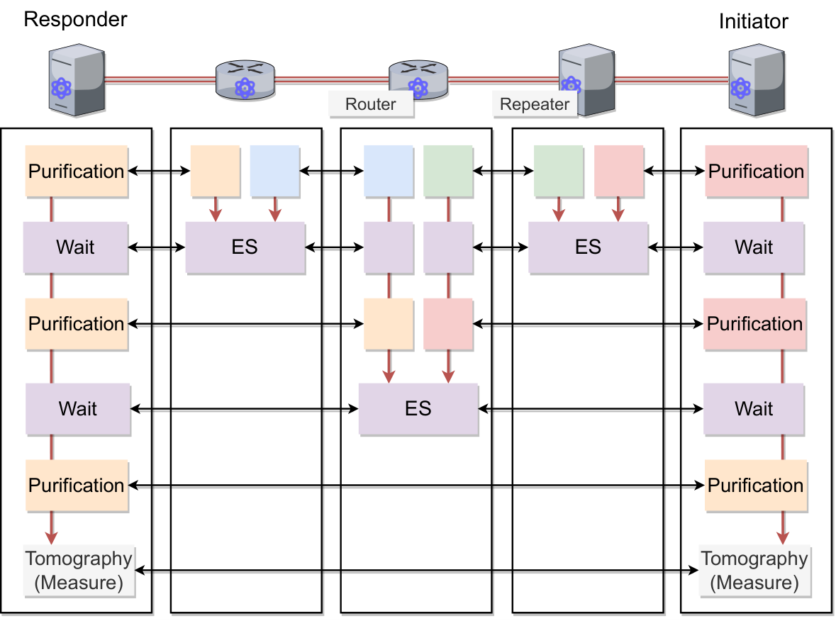
The first step in the RuleSet protocol is to distribute RuleSet to intermediate quantum repeaters.

Figure 3.3 shows how the initiator sends the request to the responder and the responder returns the RuleSets. The terms ”initiator” and ”responder” are similar to ”source” and ”destination” in classical networking. However, in the context of quantum networking, we can theoretically send quantum information in either direction once. Thus, in this paper, we distinguish these terms. In RuleSet protocols, we assume static routing that all routers have their routing table, and once the path is decided, it does not change while the repeaters are generating entanglement.
The first step in connection setup is to send the request from the initiator to the responder. In this process, the initiator describes the requirements for the entanglement in the request and sends it through the path. Second, the responder receives the request and creates RuleSets for itself and intermediate repeaters. After the RuleSets are prepared, they are sent and executed.
RuleSet is composed of a set of Rules which are instructions for quantum repeaters.
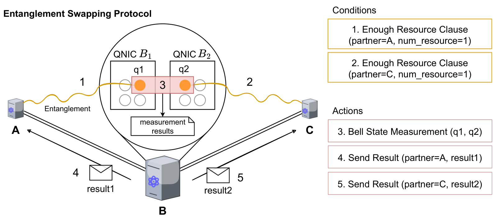
Figure 3.4 shows an example structure of a single Rule for entanglement swapping. As we showed in Section 2.7, entanglement swapping consumes two entangled states. In other words, as soon as two entangled states are ready to be used, we can move on to the measurement operation. Thus, there are two conditions called the ”Enough Resource Clause”, which is satisfied when the quantum repeater has a specified number of entangled states with a specific partner node. Once all the conditions are met, the following actions are taken. In this example, there are three actions. The first action is the ”Bell state measurement”, which takes two qubits entangled with proper partners and applies the Bell measurement to them. As a result of the measurement, repeaters can extract the results and send them to the partners.
Each rule has only pure condition clauses and action clauses so there is no way to introduce condition branching in the Rule. However, there is a concept called stage in the RuleSet. This stage allows us to divide the conditions into several different rules that can mimic the selective execution of the rules. More details on the stage system are explained in Section 4.3.2.
There are several predefined conditions and actions introduced in [13]. Table 3.1 is the list of condition clauses.
| Name | Description |
|---|---|
| Enough Resource (RES) | Check if there are enough available resources in QNIC |
| Comparison (CMP) | Compare some properties and check if that is satisfied |
| Timer (TIMER) | Check the timer is expired or not |
Enough Resource (RES) is the condition clause that checks if there are enough entangled states with sufficient fidelity. For example, if a quantum repeater A needs two entangled states with fidelity above 0.8 shared with repeater B, the condition clause is described as RES(1, 0.8, B) where the arguments correspond to
(<the number of resources>, <required fidelity>, <partner identifier>).
Comparison (CMP) checks whether a value is equal, less, or greater than some values. For instance, if we want to check the measurement result as 0 or 1, the condition clause is CMP(MeasResult, Eq, "0") where the first argument is the identifier of the classical variable. In this case, since we compare the measurement results, the variable ID is MeasResult. The second argument is the operator such as Eq(”=”), Lt(”¡”), Gt(”¿”).
Timer (TIMER) Check the timer to be expired.
Table 3.2 is the list of actions to be performed.
| Name | Description |
|---|---|
| Set Timer (SETTIMER) | Set a timer to count the time |
| Promote (PROMOTE) | Promote a resource from one rule to next |
| Free (FREE) | Free the qubit no longer used |
| Set (SET) | Set the RuleSet variable |
| Measurement (MEAS) | Measure the qubit |
| Quantum Circuit (QCIRC) | Apply quantum gates |
Set Timer starts the timer to be expired. (e.g. TIMER(10))
Promote (PROMOTE) move the ownership of the resources to the next Rule or Stage. For example, PROMOTE(qubit1, Rule2) moves a qubit which has ID (qubit1) to Rule2
(PROMOTE(<qubit id>, <Stage or Rule id>)).
Free (FREE) release the qubit ownership and reinitialize for later use. FREE(qubit123) frees the qubit with ID (qubit123) and the resource allocator starts to create link-level entanglement in the next round.
Set (SET) sets a variable to be shared in Rule, Stage, or RuleSet. For example, to count the number of measurements that occurred in a Rule, SET(MeasCount) grabs the current measurement count and updates it.
Measurement (MEAS) measures the qubit and returns the measurement result. MEAS(qubit1, X) means that measure a qubit with identifier qubit1 in X basis (MEAS(<qubit id>, <measurement basis>)).
Quantum Circuit (QCIRC) applies a series of gate operations on a qubit. QCIRC((q1, q2), (("X", q1), ("H", q2))) is an example usage of QCIRC that instructs the system to apply X gate on a qubit with ID q1 and apply H gate a qubit with ID q2. The first argument is the list of qubit identifiers and the second argument is the list of operations.
(QCIRC((<qubit id, qubit id, ..>), ((<operation>, <qubit id>), ..)))
In addition to these condition clauses and action clauses, there are also predefined protocol messages to exchange the measurement result and to notify the successful entanglement generation. Table 3.3 is the messages used in RuleSet.
| Name | Description | ||
|---|---|---|---|
| Free (FREE) | Request to free the used qubit in the partner node | ||
| Update (UPDATE) |
| ||
| Measurement (MEAS) | Tell the measurement results to the partner | ||
| Transfer (TRANSFER) |
|
3.2 Defining RuleSet
Figure 3.2 is just a very simplified visualization of the RuleSet. In reality, the RuleSet needs to be defined in some portable format. One possible way to define the RuleSet is the JSON format, which is a very common way of exchanging information between different applications.
Listing 1 shows an example definition of the RuleSet. There are several fields within the RuleSet.
- •
ruleset_id: Since RuleSet is created for the entire connection, RuleSets for one connection share the unique ids calledruleset_id. If there are multiple connections at the same time, the specific connection should be identified by thisruleset_id. - •
num_rules: This property is used to check the number of rules to be executed inside this RuleSet. - •
owner_address: The address of the owner of this RuleSet. For simplicity, this RuleSet contains integer values such asowner_address, however, this field could contain an IP address or any identifier of the specific quantum repeater or router node. - •
stages: The list of stages that contains a set of rules.
Rules also contain multiple fields.
- •
rule_id: Similarly toruleset_id, each rule also has its ownrule_id, which can be used to identify, for example, the measurement result generated by a specific rule. In the current RuleSet,rule_idis given sequentially. - •
shared_tag: This is an integer value that is shared among several rules. For example, when purification is performed on one quantum repeater, the corresponding pairs have the same shared tags. - •
next_rule_id: The identifier for the next rule. Once this rule is completed, the next rule identified by this value is to be operated. - •
condition: The list of conditions to be satisfied. - •
action: The list of actions to be operated when all conditions are satisfied.
These conditions and actions are constructed from their type and options such as the number of resources they require and the fidelity they need.
3.3 Problem Definition
As long as a large number of RuleSets are properly generated, the RuleSet protocol might be highly scalable even for quantum internetworking. However, as a user or creator of a RuleSet, it is sometimes difficult to see what is going on in a RuleSet since they are composed of a set of instructions. It is also difficult to check dependencies of Rules such as sending and waiting messages.
In this project, we propose a new domain-specific language to generate such a large number of RuleSets. In addition to that, we provide a new runtime system corresponding to that language.
Figure 3.5 gives an overview of our system. Once a network manager for this quantum network or users who want to try their protocol on the RuleSet write a .rula program and provide it to the compiler with a configuration, our system provides us a serialized RuleSet that contains a set of instructions. This system allows us to describe RuleSet in more abstract manner.
3.4 Related Works
3.4.1 Quantum Network Architectures
There are several related works on quantum networking and internet architectures. The transition from the current state of the quantum networking to scalable and a future possible quantum network stuck was introduced [40]. A similar layering model was also proposed in a different research project, however, which is more reliable by using GHZ states [88]. Higher-level routing implementation with multipartite states is also discussed.
The authors proposed entanglement generation protocols on top of the proposed layering model in [12]. They formalized entanglement tracking protocols and cutoff policies for the lifetime of entanglements.
The main target of those previous works is small to medium-scale quantum networks especially maintainable by a central node. Our scope in this protocol is further future quantum networking that is fairly less time-sensitive for the sake of longer lifetime quantum memory.
Our assumption is based on the RuleSet protocol [13] that the main proposal for quantum internet is rewriting RuleSet over the different networks. RuleSets are designed to manage quantum repeaters in an asynchronous and scalable manner.
3.4.2 Quantum Programming Language
To manipulate quantum computers through software, we need a way to describe the instructions for quantum computers. The basic compiler models for quantum computing have been introduced and surveys on programming languages for quantum computers have been conducted [89]. The various aspects such as compiler and debugger have also been discussed [90]. In the NISQ era, operation imperfection and decoherence are crucial to the computational result. NISQ quantum computer requires noise-aware circuit compilation and transpilation that produces better computational results.
In terms of the modules for existing programming languages, one of the most popular software development kits for quantum computing is Qiskit [1] from IBM. Google has also been developing its open-source quantum library called Cirq [91]. Both are modules of the Python programming language. They are modules to define quantum circuits and submit quantum circuits as jobs that can be run on real devices or simulators.
Q# [92] developed by Microsoft is a domain-specific programming language for quantum computing.
There are assembly-like languages to describe low-level gate-level instructions in quantum computing, called OpenQASM [93], which allows us to write a sequence of gate operations and measurement operations. In terms of networking, there is also a similar work that describes quantum networking operations in an assembly-like language called NetQASM [94]. The usage of NetQASM is experimentally demonstrated [95].
There is a functional programming language called Quipper that is specialized in the generation of large quantum circuits [96]. Qwire is also a programming language that defines gate-level quantum circuits [97]. Silq [98] is also a high-level programming language that can define a quantum circuit with a small number of lines. [99] introduces how the entanglement is reasoned in the computer program with a new programming language called twist.
There is also a research direction that tries to integrate classical networking technology into quantum networking. The authors are trying to use the software-defined network (SDN) technique [100]. There is also research work that is trying to integrate the manipulation of the data plane of existing p4 data into quantum networking [101].
Chapter 4 Proposal
This chapter introduces our proposal programming language that allows us to write down RuleSet in more abstract way. In Section 4.1, the required features for this language are listed. The assumptions we made are discussed in Section 4.2. The design principles of RuLa are introduced in Section 4.3 and we dived into the detailed grammar and semantics in Section 4.4. Section 4.5 covers how the RuLa program is compiled into lower-level RuleSet instructions.
4.1 Requirements
In the current RuleSet generation process, there are three possible difficulties when there are a number of Rules and RuleSet.
- 1.
Visibility: It becomes difficult to grasp what is going on in a Rule.
- 2.
Consistency: It is hard to resolve the dependencies of two dependent Rules.
- 3.
Expressibility: Multiple different Rules are needed to describe multi-condition operations.
From these possible difficulties in the current RuleSets, the requirements for RuLa are introduced as follows.
1. Visibility enhancement: The RuleSet and each Rule that is contained in a RuleSet is composed of a set of instructions shown in Table 3.1, 3.2 and 3.3. Resulting RuleSets are generally produced in a serialized format such as JSON. It is hard to see the relationship between the repeaters and the flow of the operation. RuLa must enhance the visibility of the RuleSet.
2. Automatic consistency support: When Rule A sends a message to Rule B, Rule B has to wait for the message from Rule A. In this case, Rule B has a dependency on Rule A. The RuLa compiler should support automatic consistency resolution to reduce the potential inconsistent Rule errors.
3.Support multi-conditioning: The current RuleSet does not support multi-conditioning in a Rule such as “if condition A is satisfied, do action A. If condition B is satisfied, do action B”. Instead, we need to create two different Rules with two different conditions in a single stage. RuLa should support the functionalities that translate that multi-level conditioning into a set of different Rules in a stage.
4.2 Assumptions
Since quantum computing and networking are still early-stage technologies, there is no strong consensus on the general architecture. In this section, we explain the assumptions that we made to design this language.
4.2.1 Quantum Recursive Network Architecture
One of the fundamental assumptions we made is the assumption of quantum network architecture. Our primary target architecture is the RuleSet-based Quantum Recursive Network Architecture (QRNA) [13, 102]. The network is divided into multiple layers and is recursively managed.

Figure 4.1 shows the basic idea of QRNA. The network in layer is virtualized in the higher layer . The advantage of this architecture is that higher-layer quantum repeaters are not involved in lower-layer resource management. This allows us to have independent and scalable resource management in the different layers.
4.2.2 Quantum Node Architecture
We also need some assumptions on the hardware and software architecture for quantum repeaters. A proposal of the repeater architecture is in Quantum Internet Research Group (QIRG) work in the Internet Research Task Force (IRTF) [103]. This RFC is still a draft version, but we believe that the fundamental concept of quantum networking will not change drastically in the future. In addition, we believe that the architecture based on RuleSet [14, 13] is a good candidate for future quantum networking and internetworking. Based on these architectural proposals, Figure 4.2 is the basic architecture that we assume in this project.
4.2.3 QRSA (Quantum Repeater Software Architecture)
In terms of software architecture, we assume the Quantum Repeater Software Architecture (QRSA) is the fundamental software architecture for quantum repeaters. QRSA is composed of the following components.
- •
Connection Manager: a software component that is responsible for handling requests and responses for connection setup and creating RuleSet for intermediate quantum repeaters.
- •
Hardware Monitor: a system that monitors the status of the hardware (e.g. the fidelity of the link, memory). The hardware monitor may provide that information to choose the path for routing and multiplexing.
- •
Routing Daemon: routing daemon is a daemon process that constantly updates the routing table for successful routing.
- •
Real Time Controller: a system that manipulates the hardware and receives feedback. When the Rule Engine makes a request to apply quantum gates to a qubit, Rule Engine issues a request to Real-Time Controller.
- •
Rule Engine: a critical component that handles RuleSet. Rule Engine is also responsible for managing the resources available for the Rules. Rule Engine receives RuleSet from Connection Manager and converts provided RuleSets into an executable format. The converted RuleSet instructions are executed one by one.
4.2.4 QNIC (Quantum Network Interface Card)
Classical computers and servers have one or more Network Interface Card (NIC) to communicate over the network or the Internet. In quantum networking, we assume the existence of the Quantum Network Interface Card (QNIC) which is a quantum analogue of a NIC. Inside the QNIC, there are solid quantum memories that can store quantum information. In this project, we assumed that arbitrary operations among the different QNICs in a single node can be performed without any overhead.
4.3 Design Principle
The design of syntax and grammar should describe the way to execute the execution of the RuleSet execution model. The resulting program should also be able to include device-specific configurations to support the flexibility of RuleSet definitions.
4.3.1 Target Users
The target users for this language are 1. people who want to build up quantum communication protocols in the RuleSet scheme and 2. computer systems that are responsible for RuleSet generation.
Our primary expectation is the one who wants to try a new quantum communication on a simulator or test devices that supports RuleSet processes. Thus, the grammar and syntax of RuLa should be human-readable for people to write it easily. In addition, we also expect a computer process that is responsible for RuleSet generation such as some controller devices for the quantum network could also use this language to build RuleSets for controlled devices.
4.3.2 Rule Execution Model
The rule execution process is divided into five steps.
Figure 4.3 shows how a single rule is executed.
- 1.
Check: Once at a certain time, the condition checks whether the clauses are satisfied or not. The condition checks the table of assigned Bell pairs if their status is ready to use and if the fidelity is high enough, as well as some constant variables.
- 2.
Satisfy: If all condition clauses are satisfied, the rule calls for the corresponding actions.
- 3.
Perform: The action clauses are performed one by one on the target qubit. This might include some classical operations, such as sending measurement results to the other repeaters.
- 4.
Notify: After every operation is completed, the results of the actions need to be notified to the resource manager inside the RuleEngine and the corresponding rules running on the other quantum repeaters.
- 5.
Promote: If there are resources that are moved from the previous rule to the next rule, the resource manager updates the table of the resources, and the corresponding resources are promoted.
From these items, RuLa must describe 1. What are the conditions to be satisfied, 2. How these conditions are met 3. What operations are performed, 4. How to tell the result of actions to the other rules, 5. How to transfer updated resources from one rule to another.
4.3.3 Repeater Identifications
In order to identify which repeater communicates with which other repeaters, RuLa should provide a way to specify the target repeaters. However, the RuLa program itself must be independent of the number of repeaters in the path. RuLa should offer the ways to identify the repeaters as follows.
- 1.
Identify a repeater with a specific index.
- 2.
Identify a repeater relatively with the number of hops from the target repeaters.
- 3.
Identify a repeater dynamically with the index variables.
Those three ways of identifying a repeater value allow us to specify a repeater and its partner repeaters without knowing the number of actual repeaters beforehand.
4.3.4 Compilation RuLa program
In terms of the timing that a RuLa program is compiled, the RuLa program is compiled anytime if there are RuLa programs with a user who wants to try a new protocol. In the case that a computer program generates a RuLa program for actual entanglement generation, a RuLa program is compiled when the connection setup request arrives at the responder node. The responder node compiles the RuLa program with the given repeater information and compiles a RuLa program with it.
4.4 Language
In this section, we explain the detailed language design and specifications of RuLa. The full specification is in Appendix A.
4.4.1 Grammar Definition
We chose Parsing Grammer Expression (PEG) [104] to define the grammar. PEG can define grammar rules without any ambiguity.
Let be defined expressions. Expressions follow the rules listed below in PEG.
- •
: follows immediately after .
- •
: If is not evaluated, is evaluated.
- •
?: can be omitted
- •
*: Zero or more
- •
+: One or more
It is also possible to define a new rule with .
| (4.4.1) |
where NewRule is supposed to be either Rule1 or Rule2.
To define the grammar, we used pest[105] which is a grammar rule generator based on the PEG expression.
The way to define grammar in pest is quite similar to how we define grammar in a pure PEG expression; however, there is some syntax sugar to make grammar definition easier.
As an extension of PEG, pest supports the following rules for convenience.
- •
ˆ”keyword”: Case sensitive
- •
! ”keyword”: Prohibit ”keyword”
4.4.2 Terminal Characters
The termination characters are defined as ASCII_DIGIT and ASCII_ALPHA.
There is also a rule ANY that includes symbols such as @, * as well.
4.4.3 Supported Data Types
In RuLa, there are five primitive data types that would be required for RuleSet and five composite data types to simplify data handling.
Integer: The integer value is made up of one or more than one digit of numbers.
Internally, it is converted to a 64-bit signed integer value
( to ).
In the variable definition, the integer value must be annotated with int.
Unsigned Integer: If the value is defined as an unsigned integer value, that value can be between to . ( to )
The unsigned integer variable must be annotated by u_int when it is defined.
Floating Point: The floating point value consists of an integer part, a floating point, and fraction values.
The floating-point value is converted to a 64-bit floating value internally.
( to ).
The floating-point variable must be annotated with float in the variable definition.
Boolean: The Boolean value can be true or false.
The Boolean value must be annotated with bool.
String: The string value is represented as a value quoted by double quotation (").
Some characters \ and " cannot be included in the quotation.
Vector: A vector value contains multiple data inside, but the type of data needs to be the same among all data.
Composite Data Types: For convenience, RuLa natively supports the following composite data types.
- •
Qubit (
Qubit): An alias type of the target qubit. A qubit value stores an index value that is valid in the rule definition. - •
Repeater (
Repeater): The type of quantum repeater that contains several methods to specify the partner quantum repeaters. - •
Message (
Message): The message type value stores the message contents from the other repeaters. - •
Result (
Result): The result type value stores the measurement result created by the measurement operations. - •
Time (
Time): To check if the timer has expired or not, RuLa provides Time as a primitive data structure to represent the time and check the timer expirations. In the current version, thisTimetype is not available.
4.4.4 Variable Definition
let statement allows us to define a variable as shown in Listing 2.
Variable identifiers must be properly annotated in the let statement.
4.4.5 Importing
To keep the system’s modularity, RuLa allows us to import rules and functions defined in other files. It is possible to get functions and structures from other places with import as we show in Listing 4.
Types and functions are specified using delimiters (::).
At the end of the path, it is also possible to set a list of identifiers that represent functions and structures.
4.4.6 Rule definition
Rule expression defines a rule that describes how the target repeater interacts with its qubits and other repeaters. Rule definition starts with "rule" and ident for the name of the rule. The identifier for the repeater repeater_ident follows that with angle brackets (<, >) and a set of arguments within parenthesis ((, )).
To distinguish an ordinary value and a repeater value, the repeater value has a special identifier starting with #.
The target repeater can be referred to with the given identifier within the rule.
A rule may promote a qubit value to the next rule. The ret_type_annotation is required when the rule has promote expression (see Section 4.4.16 in details).
The contents of the rule start with let statements that can define variables used within the rules.
The conditions cond_expr and actions act_expr follow them.
4.4.7 Condition Clauses
Condition expression (cond) contains multiple condition clauses to be evaluated.
4.4.8 Action Clauses
act expression describes the corresponding actions to be performed when the condition is met. Listing 8 is an example that applies Bell State Measurement to q1 and q2 which are defined in the condition clause.
4.4.9 Repeater Definition
It is possible to specify each individual repeater node in the path in the RuLa program. The very first line of the RuLa program starts with #repeaters: vec[Repeater] that contains the repeaters in the path. Figure 4.5 shows how repeaters are indexed in the #repeaters.

Each repeater can be specified by the index of #repeaters value.
For example, the first repeater can be called #repeaters(0). It is also possible to specify with some parameters (e.g. #repeaters(i+1)) for dynamic repeater selection.
4.4.10 Rule Call Expression
Calling the defined rule is done similarly to the function call, but the rule call takes an additional argument of Repeater value.
For example, the following expression prepares the swapping rule for the first repeater.
The rule is evaluated with a given repeater value.
4.4.11 RuleSet Definition
4.4.12 Conditioning
RuLa supports two types of conditioning to easily construct complex rules.
If Statement
if statement can take multiple else if statement and one else statement at the end.
if_block needs to return a Boolean value.
if statement works differently whether it is defined in the rule statement or ruleset statement.
Match Statement
Another way to define conditions is by using the expression match. In the match statement, the conditions are evaluated from top to bottom. If one of these conditions is satisfied, the corresponding actions following after => are executed. We can also define operations with otherwise in the case where all conditions are not met.
These conditioning expressions have a special ability for RuleSet generation. RuleSet originally does not allow any conditional operations in condition clauses. For example, quantum repeaters have to apply selective operations based on the Bell measurement results at other nodes. In RuleSet, those operations are achieved by preparing multiple rules in a stage.
When multiple factors are considered in the conditions, the number of rules grows. In RuLa, these conditions are automatically expanded to combinations of rules, even if there are multiple conditions. An example is shown in Figure 4.6
4.4.13 Loop
Looping is also an important functionality for most programming languages. We can define loop operations with for expression.
Listing 13 is an example for loop expression with a generated function. In this example, the numbers are substituted, and the statements inside the curly braces are evaluated.
4.4.14 Function Call Expression
To call the functions defined in the other file or another place, the following function call expression can be used.
As an argument for the function, the four types of expression can be in parentheses.
4.4.15 Send Statement
In quantum repeater networks, message exchange often appears in the process. Especially shown in Table 3.3, there are four types of defined protocol messages used to transfer a certain instruction and measurement results to the other quantum repeaters.
RuLa supports this message transfer with the -> symbol.
The function call goes to the left-hand side of the -> symbol. This function call needs to be one of four types of functions.
- •
update(<resource id>, <pauli_correction>): Apply the Pauli correction operation to the resource with<resource id>. - •
free(<resource id>): Frees the resource whose resource id is<resource id>. - •
meas(<resource id>, <measurement_result>): Send the measurement result corresponding to the<resource id>. - •
transfer(<resource id>): Notify of successful entanglement swapping and transfer a new resource id.
The right-hand side of the send expression can be any expression but needs to be a value with Repeater type.
This #repeaters vector is resolved by the configuration given in the compilation (see the details in 4.5).
4.4.16 Promoting Values
Promoting entangled resources is one important operation in the Rule definition. Right now, the only value we can promote is Qubit type values.
When a Rule contains promote statement, that rule requires type annotation.
Listing 14 shows an example type annotation when the rule contains a promote statement. In the action clauses act{...} there is a if statement that could promote a qubit value.
4.5 Compiler
The RuLa program needs to be translated into basic RuleSet instructions. Figure 4.7 is an overview of the RuLa compiler architecture.

4.5.1 Input/Output
The first input for this compiler is the source code written in RuLa. The file index of the RuLa program should be .rula, and the input program is passed to Parser. The second input is a configuration file that contains a set of properties of quantum repeaters.
Listing 15 is an example configuration of repeaters.
The configuration file is converted into a vector of Repeater values that provide some useful functions to specify the partners. As an example, it is possible to select the partner quantum repeaters with the number of hops generated by this configuration.

For example, if the repeater B in Figure 4.8 wants to specify the repeater A as a partner node, it is possible to do it with
where #rep is the variable used in the Rule to specify the target repeater (in this example, the target repeater is repeater B).
The output files are RuleSet which is serialized in JSON format. If the configuration file contains properties of five repeaters, the number of output files is also five and each RuleSet is corresponding to each repeater.
4.5.2 Parser
There are two important components in the RuLa compiler. One is a parser and the other is a code generator. The parser generates Abstract Syntax Tree (AST) from an input RuLa program. AST nodes are defined based on the grammar introduced in Section 4.4.1.
Figure 4.9 is an example of an AST structure. The definition of the rule starts from RuleExpr which consists of four different values.
- •
Name: The identifiable name of the rule.
- •
Repeater Identifier: The repeater of the identifier starts with
#. - •
Arguments: Similarly to function arguments, the rule definition can also take some arguments that are passed by when the rule is evaluated. Those arguments are also a series of identifiers.
- •
RuleContents: Finally, the actual content of the rule is expressed by
RuleContentExprwhich is made up of several important components for the definition of the rule.
The entire RuLa program is translated into a single large tree that is composed of multiple AST nodes.
4.5.3 Generator
RuLa generator translates the AST given by the parser into the Rust code [106]. Each statement and expression is corresponding to some pieces of Rust code that can generate RuleSet instructions. For example, the if statement is translated into a set of closures that describes what is the conditions to be met and the actions to be performed. Some built-in functions such as send(), free() are also converted into a set of RuleSet instructions.
This generator first generates Rust code and the generated Rust code is compiled by the Rust compiler. Some serialized RuleSets are generated as outputs of the compilation.
4.6 Examples
In this section, we introduce several examples of the RuLa programs and configurations.
4.6.1 Simple Entanglement Swapping
The first example is the simple entanglement swapping protocol shown in Listing 4.6.1.
The program starts with repeater vector definition in line 2 which stores repeater values. Line 4 imports quantum operation functions Pauli Z gate (z()), Pauli X gate (x()) and Bell State Measurement (bsm()).
A swapping rule is defined between line 6 and line 29.
swapping rule takes a repeater argument (#rep) and an integer argument distance.
Line 7 and 8 define the target partner quantum repeaters with a function called hop function which is implemented in the Repeater value.
Condition clauses are defined between line 9 and line 12. A qubit returned from res function is stored in a variable q1 that can be used in action clauses.
Action clauses are defined from line 12 to 28. Firstly, perform Bell State Measurement in line 13. According to the measurement result, send different messages to the partner repeaters (line 14 to line 24).

4.6.2 Entanglement Swapping with Purification
The following example (Listing 16) shows an example program that allows an initial purification before the entanglement swapping rule.
The second example is entanglement swapping with a single round purification. Same as the previous example, the program starts with a definition of the repeater vector in line 1.
In this example, the swapping rule defined in the different file is imported in line 4.
A local_operation rule is defined from line 6 to line 20. Same as the previous example, this rule takes a single repeater argument and an integer argument. However, since this rule contains promote statement that promotes a qubit to the next rule, the type annotation is put after the argument definition.
This example only contains one round of purification, but it is also possible to add multiple rounds of purification to the RuleSet before swapping by adding one more loop.
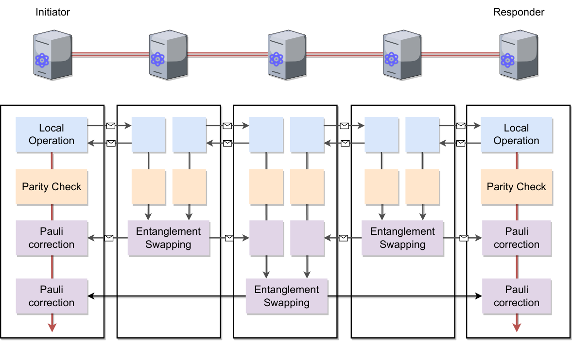
4.6.3 Entanglement Swapping with Multiple Round Purification
It is also possible to assume that all purification is done after the end-to-end entanglement is generated.
Chapter 5 Evaluation
In this chapter, we evaluate our proposal in terms of three aspects. First, we evaluate the requirements introduced 4.1 and check how RuLa satisfies those requirements in Section 5.1. Second, we explain the limitations of current RuLa in Section 5.2. Finally, we enumerate several use cases of RuLa in practical situations in Section 5.3.
5.1 Requirement Satisfaction
This section discusses whether the requirements listed in Section 4.1 are satisfied in RuLa and the coverage of the basic instructions shown in Table 3.1, 3.2 and 3.3.
5.1.1 Requirement 0: Instruction Coverage
The primitive instructions introduced in Section 3.2 must be covered by some elements in RuLa such as functions, expressions, and statements.
Condition Clauses
RES:
res(<# of resource: u_int>, <fidelity: float>,
<partner repeater: Repeater>, <index: u_int>)
res function takes four arguments. The first argument is an integer value to count the number of required resources. The second argument is a float value for threshold fidelity value. The third argument is a Repeater value that represents a partner repeater node. The final argument is an index value for the resource. This function returns a Qubit type reference to the qubit.
TIMER:
check_timer(<timer_id: str>) This function generates the condition TIMER to check if the timer has expired or not. Right now, the timer id is given by some string identifiers.
CMP:
cmp(<target: Result>, <operation: str>, <value: str>)
cmp function takes three arguments. The first argument is the Result value that can be compared to some values. operation is a set of comparison operators (e.g. ==, >).
RECV:
recv(<partner repeater: Repeater>)
recv function takes a repeater value and makes an RECV instruction based on the repeater information.
Action Clauses
SETTIMER:
set_timer(<timer_id: str>, <duration: int>)
set_timer function set a new timer with an integer duration value. A timer can be identified by a string value timer_id.
PROMOTE:
promote statement introduced in Section 4.4.16 is corresponding to the PROMOTE instruction that promotes a qubit to the next rule.
FREE:
free(<resource_id: Qubit>)
free function takes a Qubit value as an argument and issues an instruction to free that qubit.
SET:
set statement explained in
SET instruction is supported by the return expression. Once a Rule returns the value, the parent RuleSet stores the value and provides it to the other Rules. This operation corresponds to the SET operation in RuleSet.
MEAS: Measurement operations are defined in the standard library for RuLa.
measure(<qubit: Qubit>, <measurement_basis: str>) is a function to make a measurement instruction. The first argument is a Qubit value that identifies the target qubit and the second argument is the measurement basis that can be X, Y or Z
QCIRC:
A quantum gate is also defined as a function in the standard library.
For example, x(<qubit: Qubit>) make a QCIRC instruction with a qubit identifier.
Protocol messages are defined as Send expressions with the -> symbol.
- •
free(<resource_id>) -> repeaterfrees the target resource in therepeater. - •
update(<resource_id>, <pauli_correction>) -> repeaternotify the result of entanglement swapping to therepeaterwith corresponding Pauli correction operations. - •
meas(<resource_id>, <measurement_result>) -> repeatersend the raw measurement results to therepeater. - •
transfer(<resource_id>) -> repeatertell therepeaterthe successful entanglement swapping.
5.1.2 Requirement 1: Visibility Enhancement
RuLa supports the following functionalities to enhance the visibility of the entire Rule process.
Modular Rule Definition: RuLa supports import statement to get Rules defined in different files into the current RuleSet definition. This import statement improves the maintainability of the Rule definition. Users do not have to define all the required Rules in a single file that lose the visibility of the entire program.
Clear Rule definition process: The way to define the Rule is clearly divided into four steps as explained in Section 4.4.6. It is possible to see who is the owner of the Rule and who is the partner of the Rule easily and also possible to check what are the conditions and actions.
Repeater type values also provide some useful functions that contribute entire visibility, such as #rep.hop() to identify the repeater placed in a specific number of hops from the owner repeater.
RuleSet definition with Rule Call:
In the ruleset statement, the rules defined in the Rule definition process can be called in the RuleSet definition process. This allows us to see the order of the Rules and the relationship between the Rules. It is also possible to see the flow of resources from one Rule to the next Rule.
5.1.3 Requirement 2: Consistency Support
The consistency of the Rule is automatically supported in the RuLa compiler. send statement automatically resolves the two dependent Rules.
For example, a piece of code shown in Listing 5.1.3 shows a send statement that sends a free message to a repeater with a qubit identifier.
This statement is translated into the two different RuleSet instructions. The first instruction is a send instruction for the owner of this Rule. The second instruction is a wait instruction for the partner repeater.
5.1.4 Requirement 3: Expressibility Enhancement
RuLa allows us to generate RuleSets clearly and easily in terms of the following four aspects.
Condition expantion
In RuLa, match and if expressions are automatically expanded to the series of Rules within a single Stage. This allows us to set multiple complex conditions easier than defining each of them. For example, if there are two match expressions with four conditions in a Rule, the number of Rules at the end of two match expressions is .
Dynamic Repeater Selection
RuLa supports natively the Repeater type and useful methods for repeater values. This allows us to specify the partner repeater nodes dynamically and easily.
Type checks for promoted values There might be a promotion operation in a Rule. The type of promoted value and given value from the previous rule need to be consistent. RuLa supports type checks for the promoted values and if there are inconsistent promotions between the Rules, RuLa spits out compile errors.
5.2 Limitations
In this project, we made some assumptions that should be removed in the future. These assumptions result in the limitations of RuLa.
5.2.1 RuleSet Generation
We enumerate several limitations on the RuleSet generation process.
Limitation 1: RuleSet is done statically: Since all RuleSets are created in the responder node, the responder node must know the intermediate device topologies before the RuleSet creation. Thus, a specific path must be established with some policies, and that path cannot be changed until the entanglement generation is done. This assumption might lose the robustness of the entire process when an intermediate repeater had some trouble with the generation process. The biggest issue with this assumption is that we cannot flexibly change the number of rounds of purification and error correction based on the required fidelity and the state of the fiber.
In terms of the operations inside the RuleSet, it is possible to give some conditions for semi-dynamic operations (e.g. do measurements based on the result). However, the RuleSet needs to describe all possible combinations of operations to be fully functional.
Limitation 2: The primary target state is the bipartite state: Related to limitation 1, the current target quantum state is all bipartite state because the multipartite state might require a more complex routing table. It is still possible to handle the GHZ state in a straight line without any branching but it is difficult to generate a complex graph state in the current system. Especially in the network-level entangled states, this assumption is fairly acceptable in the near future. However, there will be a demand for multipartite state communication in the future.
5.2.2 Optimizations
We consider possible future optimizations.
Optimization 1: RuleSet generation for heterogeneous quantum network When it comes to heterogeneous quantum networks as shown in Figure 5.1, there might be operation time differences between the different physical systems. For example, the gate time of the linear optical quantum repeater network tends to be faster than that of any other physical system. When we think of the combination of linear optical quantum repeaters and trapped ion quantum repeaters, the linear optical quantum repeaters have to wait for trapped ion repeaters to finish entanglement generation.

The possible direction of optimization to solve this problem is to put some TIMER operations to align the operations.
Optimization 2: Link property adaptive RuleSet generation In the current RuleSet scheme, it is not possible to generate dynamically by considering the link cost between repeaters. For example, if there is a bad link whose fidelity of the link-level entanglement is 0.8 and there is another link whose fidelity of the link-level entanglement is 0.95. In this case, the number of required entanglement purification would be different (e.g. the first link requires three rounds of purification and the second link requires one round of purification). Their error characteristics are also different (e.g. the first link-level entanglement tends to have X error but the second link-level entanglement does not).
One possible solution to deal with this situation is to use some variables that represent link-specific parameters and process them in the RuLa compiler.
5.3 Use Cases
In this section, we discuss several use cases of RuLa.
Use case 1: Protocol testing: The first use case is to accelerate protocol development for quantum networking by making the RuleSet creation process easier (Figure 5.2 shows a cycle of protocol creation with RuLa). The first step of protocol testing is to create a RuLa program that describes how a new protocol works. After writing the program, users prepare a configuration and give it to the RuLa compiler with the written program. RuLa compiler gives users the ability to deserialize RuleSets that can be tested on the RuleSet-based simulator (e.g. QuISP [107]) or actual devices that support RuleSet execution. As a result of the execution, users could obtain the final fidelity of the generated quantum states or other performance indices that can be used to evaluate the performance of the protocol. Based on those performance tests, users might come up with a better structure of protocols and test again without touching the raw RuleSets.
Use case 2: Network management: The second use case is network management, shown in Figure 5.3.

Depending on the type of application, we might prepare for entanglement with different fidelities. For example, QKD might require 98% fidelity Bell pairs to increase the key generation rate, but DQC might require Bell pairs with 99.999% fidelity to ensure greater reliability. This strategy differs depending on the applications. In that case, it takes time to generate the corresponding RuleSets from scratch.
If the responder node has multiple RuLa programs according to the applications or the fidelity of the states, the RuLa program works as if the policy of the entanglement generation. Responder receives the intermediate repeater information and recompiles the prepared RuLa programs with the configuration and distributes generated RuleSets to the intermediate repeaters.
Chapter 6 Conclusion
6.1 Conclusion
In this thesis, we presented a new programming language RuLa for RuleSet-based quantum repeaters. RuLa is the first programming language for RuleSet-based quantum repeaters, which allows us to create RuleSets in a very straightforward way. We formulate the requirements for the RuLa as these three things.
The first requirement is reliable and scalable RuleSet generation. RuLa supports higher-level conditioning and looping which allow us to generate many Rules at the same time. There is also a way to specify a partner repeater dynamically. These functionalities give us the ability towards scalable RuleSet generation.
The second requirement is the coverage of the RuleSet instructions. RuLa covers all the instructions supported in the RuleSet with statements, expressions, and built-in functions.
The third requirement is that RuLa should make RuleSet definition clearer and easier. In terms of clearance, RuLa follows the order of the Rule execution. This means that it is possible to understand the programs in the way that is executed.
We also mentioned the limitation of the current RuLa. In RuLa, since all the information for the repeaters is given before the execution, no dynamic RuleSet generation can be done such as deciding operations based on the current fidelity of the link. However, it is still possible to prepare several RuLa programs in one place and choose one of them based on the requirements for the application. In addition, RuLa does not care about the lower-level physical architectures which would be another source of errors and increase the waiting time. These limitations are the tasks that should be solved in a future version.
Finally, we also enumerated two use cases of RuLa. The first use case is to accelerate the testing of a new protocol. Since writing RuleSet became easier, it is possible to test and update a RuleSet for a new protocol easier and faster. The second use case is the selective RuleSet generation based on the applications.
This thesis explained the motivations to use RuLa and how RuLa is implemented. We believe that RuLa advances quantum networking research.
6.2 Future Work
In future works of this project, this approach should be more general to support internetworking. Currently, RuleSet generation is assumed to be done in a single network. However, we should be able to handle internetworking RuleSet generation.
It is also important for RuLa to show more examples and test them in an actual simulator which would give us more confidence that the entire system works properly.
In terms of language design, we might need more theoretical discussion such as Turing completeness, livelock, and deadlock.
6.3 Availability
The source code is available on GitHub (https://github.com/Chibikuri/rula)
Bibliography
- [1] Andrew Cross. The ibm q experience and qiskit open-source quantum computing software. In APS March meeting abstracts, volume 2018, pages L58–003, 2018.
- [2] Frank Arute, Kunal Arya, Ryan Babbush, Dave Bacon, Joseph C Bardin, Rami Barends, Rupak Biswas, Sergio Boixo, Fernando GSL Brandao, David A Buell, et al. Quantum supremacy using a programmable superconducting processor. Nature, 574(7779):505–510, 2019.
- [3] Yiqing Zhou, E Miles Stoudenmire, and Xavier Waintal. What limits the simulation of quantum computers? Physical Review X, 10(4):041038, 2020.
- [4] Charles H Bennett, Gilles Brassard, Claude Crépeau, Richard Jozsa, Asher Peres, and William K Wootters. Teleporting an unknown quantum state via dual classical and einstein-podolsky-rosen channels. Physical review letters, 70(13):1895, 1993.
- [5] Anocha Yimsiriwattana and Samuel J Lomonaco Jr. Distributed quantum computing: A distributed shor algorithm. In Quantum Information and Computation II, volume 5436, pages 360–372. SPIE, 2004.
- [6] Artur K Ekert. Quantum cryptography and bell’s theorem. In Quantum Measurements in Optics, pages 413–418. Springer, 1992.
- [7] Vittorio Giovannetti, Seth Lloyd, and Lorenzo Maccone. Advances in quantum metrology. Nature photonics, 5(4):222–229, 2011.
- [8] Peter C Humphreys, Norbert Kalb, Jaco PJ Morits, Raymond N Schouten, Raymond FL Vermeulen, Daniel J Twitchen, Matthew Markham, and Ronald Hanson. Deterministic delivery of remote entanglement on a quantum network. Nature, 558(7709):268–273, 2018.
- [9] Bas Hensen, Norbert Kalb, MS Blok, AE Dréau, Andreas Reiserer, RFL Vermeulen, RN Schouten, M Markham, DJ Twitchen, Kenneth Goodenough, et al. Loophole-free bell test using electron spins in diamond: second experiment and additional analysis. Scientific reports, 6(1):1–11, 2016.
- [10] Y-W Cho, GT Campbell, JL Everett, J Bernu, DB Higginbottom, MT Cao, J Geng, NP Robins, PK Lam, and BC Buchler. Highly efficient optical quantum memory with long coherence time in cold atoms. Optica, 3(1):100–107, 2016.
- [11] Ye Wang, Mark Um, Junhua Zhang, Shuoming An, Ming Lyu, Jing-Ning Zhang, L-M Duan, Dahyun Yum, and Kihwan Kim. Single-qubit quantum memory exceeding ten-minute coherence time. Nature Photonics, 11(10):646–650, 2017.
- [12] Wojciech Kozlowski, Axel Dahlberg, and Stephanie Wehner. Designing a quantum network protocol. In Proceedings of the 16th International Conference on emerging Networking EXperiments and Technologies, pages 1–16, 2020.
- [13] Rodney Van Meter, Ryosuke Satoh, Naphan Benchasattabuse, Takaaki Matsuo, Michal Hajdušek, Takahiko Satoh, Shota Nagayama, and Shigeya Suzuki. A quantum internet architecture. arXiv preprint arXiv:2112.07092, 2021.
- [14] Takaaki Matsuo, Clément Durand, and Rodney Van Meter. Quantum link bootstrapping using a ruleset-based communication protocol. Physical Review A, 100(5):052320, 2019.
- [15] Richard P Feynman. Simulating physics with computers. International journal of theoretical physics, 21(6/7):467–488, 1982.
- [16] Katherine L Brown, William J Munro, and Vivien M Kendon. Using quantum computers for quantum simulation. Entropy, 12(11):2268–2307, 2010.
- [17] Peter JJ O’Malley, Ryan Babbush, Ian D Kivlichan, Jonathan Romero, Jarrod R McClean, Rami Barends, Julian Kelly, Pedram Roushan, Andrew Tranter, Nan Ding, et al. Scalable quantum simulation of molecular energies. Physical Review X, 6(3):031007, 2016.
- [18] Abhinav Kandala, Antonio Mezzacapo, Kristan Temme, Maika Takita, Markus Brink, Jerry M Chow, and Jay M Gambetta. Hardware-efficient variational quantum eigensolver for small molecules and quantum magnets. nature, 549(7671):242–246, 2017.
- [19] Yasunobu Nakamura, Yu A Pashkin, and JS Tsai. Coherent control of macroscopic quantum states in a single-cooper-pair box. nature, 398(6730):786–788, 1999.
- [20] Pieter Kok, WJ Munro, Kae Nemoto, TC Ralph, Jonathan P Dowling, and GJ Milburn. Linear optical quantum computing. arXiv preprint quant-ph/0512071, 57, 2006.
- [21] Pieter Kok, William J Munro, Kae Nemoto, Timothy C Ralph, Jonathan P Dowling, and Gerard J Milburn. Linear optical quantum computing with photonic qubits. Reviews of modern physics, 79(1):135, 2007.
- [22] Philipp Schindler, Daniel Nigg, Thomas Monz, Julio T Barreiro, Esteban Martinez, Shannon X Wang, Stephan Quint, Matthias F Brandl, Volckmar Nebendahl, Christian F Roos, et al. A quantum information processor with trapped ions. New Journal of Physics, 15(12):123012, 2013.
- [23] John Preskill. Quantum computing in the nisq era and beyond. Quantum, 2:79, 2018.
- [24] Han-Sen Zhong, Hui Wang, Yu-Hao Deng, Ming-Cheng Chen, Li-Chao Peng, Yi-Han Luo, Jian Qin, Dian Wu, Xing Ding, Yi Hu, et al. Quantum computational advantage using photons. Science, 370(6523):1460–1463, 2020.
- [25] Bas Hensen, Hannes Bernien, Anaïs E Dréau, Andreas Reiserer, Norbert Kalb, Machiel S Blok, Just Ruitenberg, Raymond FL Vermeulen, Raymond N Schouten, Carlos Abellán, et al. Loophole-free bell inequality violation using electron spins separated by 1.3 kilometres. Nature, 526(7575):682–686, 2015.
- [26] Sheng-Kai Liao, Wen-Qi Cai, Wei-Yue Liu, Liang Zhang, Yang Li, Ji-Gang Ren, Juan Yin, Qi Shen, Yuan Cao, Zheng-Ping Li, et al. Satellite-to-ground quantum key distribution. Nature, 549(7670):43–47, 2017.
- [27] Paul Adrien Maurice Dirac. A new notation for quantum mechanics. In Mathematical Proceedings of the Cambridge Philosophical Society, volume 35, pages 416–418. Cambridge University Press, 1939.
- [28] The Qiskit Team. Representing qubit states, Jun 2021.
- [29] Jens Koch, M Yu Terri, Jay Gambetta, Andrew A Houck, David I Schuster, Johannes Majer, Alexandre Blais, Michel H Devoret, Steven M Girvin, and Robert J Schoelkopf. Charge-insensitive qubit design derived from the cooper pair box. Physical Review A, 76(4):042319, 2007.
- [30] Nicolai Friis, Oliver Marty, Christine Maier, Cornelius Hempel, Milan Holzäpfel, Petar Jurcevic, Martin B Plenio, Marcus Huber, Christian Roos, Rainer Blatt, et al. Observation of entangled states of a fully controlled 20-qubit system. Physical Review X, 8(2):021012, 2018.
- [31] Emanuel Knill, Raymond Laflamme, and Gerald J Milburn. A scheme for efficient quantum computation with linear optics. nature, 409(6816):46–52, 2001.
- [32] David P DiVincenzo. The physical implementation of quantum computation. Fortschritte der Physik: Progress of Physics, 48(9-11):771–783, 2000.
- [33] Lilian Childress and Ronald Hanson. Diamond nv centers for quantum computing and quantum networks. MRS bulletin, 38(2):134–138, 2013.
- [34] N Leung, Y Lu, S Chakram, RK Naik, N Earnest, R Ma, K Jacobs, AN Cleland, and DI Schuster. Deterministic bidirectional communication and remote entanglement generation between superconducting qubits. npj quantum information, 5(1):1–5, 2019.
- [35] Daniel M Greenberger, Michael A Horne, and Anton Zeilinger. Going beyond bell’s theorem. In Bell’s theorem, quantum theory and conceptions of the universe, pages 69–72. Springer, 1989.
- [36] John S Bell and John Stewart Bell. Speakable and unspeakable in quantum mechanics: Collected papers on quantum philosophy. Cambridge university press, 2004.
- [37] John S Bell. On the einstein podolsky rosen paradox. Physics Physique Fizika, 1(3):195, 1964.
- [38] Craig Gidney and Martin Ekerå. How to factor 2048 bit rsa integers in 8 hours using 20 million noisy qubits. Quantum, 5:433, 2021.
- [39] Rodney Van Meter, WJ Munro, Kae Nemoto, and Kohei M Itoh. Arithmetic on a distributed-memory quantum multicomputer. ACM Journal on Emerging Technologies in Computing Systems (JETC), 3(4):1–23, 2008.
- [40] Stephanie Wehner, David Elkouss, and Ronald Hanson. Quantum internet: A vision for the road ahead. Science, 362(6412):eaam9288, 2018.
- [41] Xiaoliang Wu, Alexander Kolar, Joaquin Chung, Dong Jin, Tian Zhong, Rajkumar Kettimuthu, and Martin Suchara. Sequence: a customizable discrete-event simulator of quantum networks. Quantum Science and Technology, 6(4):045027, 2021.
- [42] Daniele Cuomo, Marcello Caleffi, and Angela Sara Cacciapuoti. Towards a distributed quantum computing ecosystem. IET Quantum Communication, 1(1):3–8, 2020.
- [43] Stephen DiAdamo, Marco Ghibaudi, and James Cruise. Distributed quantum computing and network control for accelerated vqe. arXiv preprint arXiv:2101.02504, 2021.
- [44] Charles H Bennett and Gilles Brassard. Quantum cryptography: Public key distribution and coin tossing. Proceedings of the IEEE International Conference on Computers, Systems and Signal Processing, Bangalore, India, 1985.
- [45] Ronald L Rivest, Adi Shamir, and Leonard Adleman. A method for obtaining digital signatures and public-key cryptosystems. Communications of the ACM, 21(2):120–126, 1978.
- [46] Peter W Shor. Polynomial-time algorithms for prime factorization and discrete logarithms on a quantum computer. SIAM review, 41(2):303–332, 1999.
- [47] William K Wootters and Wojciech H Zurek. A single quantum cannot be cloned. Nature, 299(5886):802–803, 1982.
- [48] Hoi-Kwong Lo and Hoi Fung Chau. Unconditional security of quantum key distribution over arbitrarily long distances. science, 283(5410):2050–2056, 1999.
- [49] Peter W Shor and John Preskill. Simple proof of security of the bb84 quantum key distribution protocol. Physical review letters, 85(2):441, 2000.
- [50] Hoi-Kwong Lo, Xiongfeng Ma, and Kai Chen. Decoy state quantum key distribution. Physical review letters, 94(23):230504, 2005.
- [51] Jesús Rubio, Paul A Knott, Timothy J Proctor, and Jacob A Dunningham. Quantum sensing networks for the estimation of linear functions. Journal of Physics A: Mathematical and Theoretical, 53(34):344001, 2020.
- [52] Roman Schnabel, Nergis Mavalvala, David E McClelland, and Ping K Lam. Quantum metrology for gravitational wave astronomy. Nature communications, 1(1):1–10, 2010.
- [53] Sreraman Muralidharan, Linshu Li, Jungsang Kim, Norbert Lütkenhaus, Mikhail D Lukin, and Liang Jiang. Optimal architectures for long distance quantum communication. Scientific reports, 6(1):1–10, 2016.
- [54] Koji Azuma, Kiyoshi Tamaki, and Hoi-Kwong Lo. All-photonic quantum repeaters. Nature communications, 6(1):1–7, 2015.
- [55] Donovan Buterakos, Edwin Barnes, and Sophia E Economou. Deterministic generation of all-photonic quantum repeaters from solid-state emitters. Physical Review X, 7(4):041023, 2017.
- [56] Antonio Russo, Edwin Barnes, and Sophia E Economou. Photonic graph state generation from quantum dots and color centers for quantum communications. Physical Review B, 98(8):085303, 2018.
- [57] Yuan Lee, Eric Bersin, Axel Dahlberg, Stephanie Wehner, and Dirk Englund. A quantum router architecture for high-fidelity entanglement flows in quantum networks. npj Quantum Information, 8(1):1–8, 2022.
- [58] Masahito Hayashi, Kazuo Iwama, Harumichi Nishimura, Rudy Raymond, and Shigeru Yamashita. Quantum network coding. In Annual Symposium on Theoretical Aspects of Computer Science, pages 610–621. Springer, 2007.
- [59] Michael Epping, Hermann Kampermann, and Dagmar Bruss. Robust entanglement distribution via quantum network coding. New Journal of Physics, 18(10):103052, 2016.
- [60] Eddie Schoute, Laura Mancinska, Tanvirul Islam, Iordanis Kerenidis, and Stephanie Wehner. Shortcuts to quantum network routing. arXiv preprint arXiv:1610.05238, 2016.
- [61] Frederik Hahn, A Pappa, and Jens Eisert. Quantum network routing and local complementation. npj Quantum Information, 5(1):1–7, 2019.
- [62] Alexander I Lvovsky, Barry C Sanders, and Wolfgang Tittel. Optical quantum memory. Nature photonics, 3(12):706–714, 2009.
- [63] Wui Seng Leong, Mingjie Xin, Chang Huang, Zilong Chen, and Shau-Yu Lan. Long light storage time in an optical fiber. Physical Review Research, 2(3):033320, 2020.
- [64] Yu Ma, You-Zhi Ma, Zong-Quan Zhou, Chuan-Feng Li, and Guang-Can Guo. One-hour coherent optical storage in an atomic frequency comb memory. Nature communications, 12(1):1–6, 2021.
- [65] Kazuya Niizeki, Daisuke Yoshida, Ko Ito, Ippei Nakamura, Nobuyuki Takei, Kotaro Okamura, Ming-Yang Zheng, Xiu-Ping Xie, and Tomoyuki Horikiri. Two-photon comb with wavelength conversion and 20-km distribution for quantum communication. Communications Physics, 3(1):1–7, 2020.
- [66] Juan Yin, Yuan Cao, Yu-Huai Li, Sheng-Kai Liao, Liang Zhang, Ji-Gang Ren, Wen-Qi Cai, Wei-Yue Liu, Bo Li, Hui Dai, et al. Satellite-based entanglement distribution over 1200 kilometers. Science, 356(6343):1140–1144, 2017.
- [67] Sheng-Kai Liao, Wen-Qi Cai, Johannes Handsteiner, Bo Liu, Juan Yin, Liang Zhang, Dominik Rauch, Matthias Fink, Ji-Gang Ren, Wei-Yue Liu, et al. Satellite-relayed intercontinental quantum network. Physical review letters, 120(3):030501, 2018.
- [68] Michael Schirber. Quantum drones take flight. Physics, 14:7, 2021.
- [69] Charles H Bennett, Gilles Brassard, Sandu Popescu, Benjamin Schumacher, John A Smolin, and William K Wootters. Purification of noisy entanglement and faithful teleportation via noisy channels. Physical review letters, 76(5):722, 1996.
- [70] Keisuke Fujii and Katsuji Yamamoto. Entanglement purification with double selection. Physical Review A, 80(4):042308, 2009.
- [71] Hans Aschauer, Wolfgang Dür, and H-J Briegel. Multiparticle entanglement purification for two-colorable graph states. Physical Review A, 71(1):012319, 2005.
- [72] Caroline Kruszynska, Akimasa Miyake, Hans J Briegel, and Wolfgang Dür. Entanglement purification protocols for all graph states. Physical Review A, 74(5):052316, 2006.
- [73] Wolfgang Dür and H-J Briegel. Entanglement purification for quantum computation. Physical review letters, 90(6):067901, 2003.
- [74] Erik Hostens, Jeroen Dehaene, and Bart De Moor. Hashing protocol for distilling multipartite calderbank-shor-steane states. Physical Review A, 73(4):042316, 2006.
- [75] Jian-Wei Pan, Sara Gasparoni, Rupert Ursin, Gregor Weihs, and Anton Zeilinger. Experimental entanglement purification of arbitrary unknown states. Nature, 423(6938):417–422, 2003.
- [76] Haoxiong Yan, Youpeng Zhong, Hung-Shen Chang, Audrey Bienfait, Ming-Han Chou, Christopher R Conner, Étienne Dumur, Joel Grebel, Rhys G Povey, and Andrew N Cleland. Entanglement purification and protection in a superconducting quantum network. arXiv preprint arXiv:2201.10679, 2022.
- [77] Youpeng Zhong, Hung-Shen Chang, Audrey Bienfait, Étienne Dumur, Ming-Han Chou, Christopher R Conner, Joel Grebel, Rhys G Povey, Haoxiong Yan, David I Schuster, et al. Deterministic multi-qubit entanglement in a quantum network. Nature, 590(7847):571–575, 2021.
- [78] Dik Bouwmeester, Jian-Wei Pan, Klaus Mattle, Manfred Eibl, Harald Weinfurter, and Anton Zeilinger. Experimental quantum teleportation. Nature, 390(6660):575–579, 1997.
- [79] Akira Furusawa, Jens Lykke Sørensen, Samuel L Braunstein, Christopher A Fuchs, H Jeff Kimble, and Eugene S Polzik. Unconditional quantum teleportation. science, 282(5389):706–709, 1998.
- [80] Hiroki Takesue, Shellee D Dyer, Martin J Stevens, Varun Verma, Richard P Mirin, and Sae Woo Nam. Quantum teleportation over 100 km of fiber using highly efficient superconducting nanowire single-photon detectors. Optica, 2(10):832–835, 2015.
- [81] Ji-Gang Ren, Ping Xu, Hai-Lin Yong, Liang Zhang, Sheng-Kai Liao, Juan Yin, Wei-Yue Liu, Wen-Qi Cai, Meng Yang, Li Li, et al. Ground-to-satellite quantum teleportation. Nature, 549(7670):70–73, 2017.
- [82] Jian-Wei Pan, Dik Bouwmeester, Harald Weinfurter, and Anton Zeilinger. Experimental entanglement swapping: entangling photons that never interacted. Physical review letters, 80(18):3891, 1998.
- [83] Xiao-song Ma, Stefan Zotter, Johannes Kofler, Rupert Ursin, Thomas Jennewein, Časlav Brukner, and Anton Zeilinger. Experimental delayed-choice entanglement swapping. Nature Physics, 8(6):479–484, 2012.
- [84] Rui-Bo Jin, Masahiro Takeoka, Utako Takagi, Ryosuke Shimizu, and Masahide Sasaki. Highly efficient entanglement swapping and teleportation at telecom wavelength. Scientific reports, 5(1):1–7, 2015.
- [85] Andrew Steane. Multiple-particle interference and quantum error correction. Proceedings of the Royal Society of London. Series A: Mathematical, Physical and Engineering Sciences, 452(1954):2551–2577, 1996.
- [86] Pat Bosshart, Dan Daly, Glen Gibb, Martin Izzard, Nick McKeown, Jennifer Rexford, Cole Schlesinger, Dan Talayco, Amin Vahdat, George Varghese, et al. P4: Programming protocol-independent packet processors. ACM SIGCOMM Computer Communication Review, 44(3):87–95, 2014.
- [87] Mihir Pant, Hari Krovi, Don Towsley, Leandros Tassiulas, Liang Jiang, Prithwish Basu, Dirk Englund, and Saikat Guha. Routing entanglement in the quantum internet. npj Quantum Information, 5(1):1–9, 2019.
- [88] Alexander Pirker and Wolfgang Dür. A quantum network stack and protocols for reliable entanglement-based networks. New Journal of Physics, 21(3):033003, 2019.
- [89] Frederic T Chong, Diana Franklin, and Margaret Martonosi. Programming languages and compiler design for realistic quantum hardware. Nature, 549(7671):180–187, 2017.
- [90] Michele Mosca, Martin Roetteler, and Peter Selinger. Quantum Programming Languages (Dagstuhl Seminar 18381). Dagstuhl Reports, 8(9):112–132, 2019.
- [91] Cirq Developers. Cirq, apr 2022. See full list of authors on Github: https://github.com/quantumlib/Cirq/graphs/contributors.
- [92] Krysta Svore, Alan Geller, Matthias Troyer, John Azariah, Christopher Granade, Bettina Heim, Vadym Kliuchnikov, Mariia Mykhailova, Andres Paz, and Martin Roetteler. Q# enabling scalable quantum computing and development with a high-level dsl. In Proceedings of the real world domain specific languages workshop 2018, pages 1–10, 2018.
- [93] Andrew W Cross, Lev S Bishop, John A Smolin, and Jay M Gambetta. Open quantum assembly language. arXiv preprint arXiv:1707.03429, 2017.
- [94] Axel Dahlberg, Bart van der Vecht, Carlo Delle Donne, Matthew Skrzypczyk, Ingmar te Raa, Wojciech Kozlowski, and Stephanie Wehner. Netqasm-a low-level instruction set architecture for hybrid quantum-classical programs in a quantum internet. Quantum Science and Technology, 2022.
- [95] Matteo Pompili, Carlo Delle Donne, Ingmar te Raa, Bart van der Vecht, Matthew Skrzypczyk, Guilherme Ferreira, Lisa de Kluijver, Arian J Stolk, Sophie LN Hermans, Przemysław Pawełczak, et al. Experimental demonstration of entanglement delivery using a quantum network stack. arXiv preprint arXiv:2111.11332, 2021.
- [96] Alexander S Green, Peter LeFanu Lumsdaine, Neil J Ross, Peter Selinger, and Benoît Valiron. Quipper: a scalable quantum programming language. In Proceedings of the 34th ACM SIGPLAN conference on Programming language design and implementation, pages 333–342, 2013.
- [97] Jennifer Paykin, Robert Rand, and Steve Zdancewic. Qwire: a core language for quantum circuits. ACM SIGPLAN Notices, 52(1):846–858, 2017.
- [98] Benjamin Bichsel, Maximilian Baader, Timon Gehr, and Martin Vechev. Silq: A high-level quantum language with safe uncomputation and intuitive semantics. In Proceedings of the 41st ACM SIGPLAN Conference on Programming Language Design and Implementation, pages 286–300, 2020.
- [99] Charles Yuan, Christopher McNally, and Michael Carbin. Twist: sound reasoning for purity and entanglement in quantum programs. Proceedings of the ACM on Programming Languages, 6(POPL):1–32, 2022.
- [100] Travis S Humble, Ronald J Sadlier, Brian P Williams, and Ryan C Prout. Software-defined quantum network switching. In Disruptive Technologies in Information Sciences, volume 10652, pages 72–79. SPIE, 2018.
- [101] Wojciech Kozlowski, Fernando Kuipers, and Stephanie Wehner. A p4 data plane for the quantum internet. In Proceedings of the 3rd P4 Workshop in Europe, pages 49–51, 2020.
- [102] Rodney Van Meter, Joe Touch, and Clare Horsman. Recursive quantum repeater networks. arXiv preprint arXiv:1105.1238, 2011.
- [103] Wojciech Kozlowski, Stephanie Wehner, Rodney Van Meter, Bruno Rijsman, Angela Sara Cacciapuoti, Marcello Caleffi, and Shota Nagayama. Architectural Principles for a Quantum Internet. Internet-Draft draft-irtf-qirg-principles-11, Internet Engineering Task Force, August 2022. Work in Progress.
- [104] Bryan Ford. Parsing expression grammars: a recognition-based syntactic foundation. In Proceedings of the 31st ACM SIGPLAN-SIGACT symposium on Principles of programming languages, pages 111–122, 2004.
- [105] pest: The elegant parser. https://github.com/pest-parser/pest.
- [106] Nicholas D Matsakis and Felix S Klock II. The rust language. In ACM SIGAda Ada Letters, volume 34, pages 103–104. ACM, 2014.
- [107] Ryosuke Satoh, Michal Hajdušek, Naphan Benchasattabuse, Shota Nagayama, Kentaro Teramoto, Takaaki Matsuo, Sara Ayman Metwalli, Poramet Pathumsoot, Takahiko Satoh, Shigeya Suzuki, and Rodney Van Meter. Quisp: a quantum internet simulation package. In 2022 IEEE International Conference on Quantum Computing and Engineering (QCE), pages 353–364, 2022.
Appendix A Full Specification of RuLa
The following Listing shows the whole PEG expressions of RuLa.
A.1 Notation
The syntax is defined by Parsing Expression Grammar (PEG). Listing 17 is an example expression with PEG.
To define a new set of non-terminated rules, <- is the operator that defines a new rule with a name.
The rules to generate PEG expressions are following.
- •
: follows immediately after .
- •
: If is not evaluated, is evaluated.
- •
?: can be omitted
- •
*: Zero or more
- •
+: One or more
The tool we used to define the PEG parser is pest [105]which provides the following extended syntax.
- •
: is not allowed here.
- •
: Explicit definition that removes all white spaces inside
- •
: Inplicit definition that is ignored from the upper rules
- •
: Case-sensitive character.
A.2 Termination
Two types of values can be terminated values.
Letters: The lower-case ASCII letters (’a’.. ’z’) and upper-case ASCII letters (’A’..’Z’) are the terminated values in letters.
Digits ASCII digits can also be terminated values.
EOI
The end of the input is defined as the EOI symbol.
ANY
There is a useful rule called ANY that contains ASCII_ALPHA, ASCII_DIGIS and also special characters such as @, _, etc.
A.3 Lexical Elements
A.3.1 Comments
Comments allow us to provide some instructions or leave notes in the program. There are two types of comments.
- •
Line comments: The notes follow two slash lines
//. - •
Cross-line comments: Comments quoted by
/*and*/.
A.3.2 Identifier
A.3.3 Keywords
The keywords which are used in other expressions are as follows.
There are also type values and literals that cannot be an identifier.
A.3.4 Operators
In order to compare the values, and do some mathematical operations, the following operators can be used.
A.3.5 Punctuation
The following braces are used as punctuations in some expressions
A.3.6 Integer Literals
In RuLa, integer values are expressed by a set of digits. There are several types of integer value definitions.
Internally, any integer values are converted to 64-bit integer values.
A.3.7 Floating Literals
Floating point values are composed of an integer part, decimal point, and fraction values.
The floating point value is also converted to a 64-bit floating point value.
A.3.8 String Literals
Define the string values, it can be done with some values quoted by double quotations ".
Since the PEG expression uses double quotations, double quotation
A.4 Variables
A variable stores a value that can be used in later expressions. A variable can be defined in the following way.
where the ident_typed is an identifier with type annotations shown in A.5.
Putting the identifier refers to the predefined identifier.
A.5 Types
In RuLa, there are five primitive data types and five composite data types.
A.5.1 Boolean Type
A.5.2 Numeric Type
There are two kinds of integer types int and u_int and one type for floating value float.
A.5.3 String Type
A string type is a set of string values that are surrounded by double quotations ".
String type value is annotated by str.
A.5.4 Vector Type
A vector type contains a set of values that is annotated by vec[<inner_type>] where <inner_type> can be types values such as int, bool.
A.5.5 Repeater Type
In RuLa, the repeater can be represented as a Repeater type value.
Repeaters are special values in RuLa. All RuLa programs start with #repeaters: vec[Repeater] which stores the target repeater values generated from the configuration.
The repeater value contains the name and index of the repeaters. Figure 4.5 shows how repeater indices are assigned.
The target repeater can be called from the repeater vector #repeater(<index>) where the <index> is the index of the repeater in the path.
A.5.6 Qubit Type
Qubit type is just an alias of the target qubit. Since the actual qubit value can only be resolved when the RuleSet is executed, the qubit data type can only hold the index or identifier of the qubit within a single Rule.
For example, if one Rule consumes two qubits, these qubits are necessary to be distinguishable. When a qubit value is initialized, an index value can be assigned.
A.5.7 Result Type
Result type is a composite data type that is used to store measurement results and to make comparisons with specific values with the target measurement result. Since many measurement operations happen in quantum computing, values with result type can be used in match or if as a condition.
A.6 Expressions and Statements
RuLa supports the following expressions.
A.6.1 Function Call Expression
Functions can be called by their names.
The arguments are surrounded by the ( and ) with commas ,.
A.6.2 Rule Call Expression
Defined rules can be called by a rule-call expression.
The rule can be identified by an ident and a repeater argument repeater_call and a set of arguments fn_call_args.
A.6.3 Get Expression
get expression is to get the value registered by the set statement.
The identifier must be set properly before the get expression is called. Otherwise, the
A.6.4 Comp Expression
The value can be compared with comparison operators, and the comparison value returns a Boolean value.
A.6.5 Term expression
The numbers can be added, subtracted, multiplied, or divided from the other numbers.
A.6.6 Variable Call Expression
When the functions or variables in a composite-type variable are called, those variables and functions can be referred to with ..
A.6.7 Vector
A vector can be defined as the following expressions.
A vector can store a set of literal expressions. However, the type of literal value must be a single literal type.
A.6.8 Tuple
A tuple works similarly to the vector value. However, a tuple value can contain arbitrary expressions.
A.6.9 Literal Expression
The literal expressions can be defined as follows.
A.6.10 Statement
A.6.11 Import Statement
To keep the modularity of the rules and functions, RuLa supports importing other rules and functions.
A set of identifiers and delimiter :: represent the position of the file, function, and rules.
A.6.12 Rule Statement
Rule statement allows us to define independent rules.
The rule statement is composed of five different components. The first ident is the name of the target rule and the repeater_ident is an identifier for the target rule.
In the rule definition, the repeaters can be referred to with a special identifier starting with #.
Then the argument definition and type annotations are following after that.
In the rule contents, there are four different components.
The first series of let statements are used to define values that live till the end of the rule.
cond_expr defines a set of conditions to be satisfied.
There are three possible candidates for the condition clauses. The first res_assign assigns a generated value by a function and passes it to the action clauses. The other two are fn_call_expr and variable_call_expr.
action+expr defines a set of actions to be performed when the conditions are met.
A.6.13 RuleSet Statement
At the end of the program, the ruleset can be defined with ruleset statement.
When the defined rule is called in this statement, a created rule is stored in the ruleset.
The ident follows "ruleset" is the name of the ruleset.
A.6.14 Let Statement
A let statement is a statement that defines a new variable.
Let statement requires a typed identifier as a left-hand side value. It is also possible to put multiple typed identifiers surrounded by ( and ).
A.6.15 Match Statement
The match statement supports higher-level conditioning for generating complex rules.
match statement expands multiple conditions to multiple different rules in a single stage. Figure 4.6 shows how the match is expanded to the different rules in a single stage. The top expression for matching needs to be comparable with literal values.
A.6.16 If Statement
If the statement works similarly to the match statement but it can explain more complex conditioning.
In the rule statement, this if statement is also expanded to the multiple different rules in a stage.
A.6.17 For Statement
for statement takes one by one from the given expression.
One or multiple temporary variables follow after "for". After these identifiers, "in" and the corresponding expression follow.
In the statements in for, it is possible to use defined identifiers as ordinary identifiers.
A.6.18 Promote Statement
In order to promote a resource from one rule to the next rule, promote statement returns a value to a parent ruleset and makes it available for later rules.
Currently, the promotable value must be a Qubit type value.
A.6.19 Set Statement
In order to share the values other than the Qubit type value, set statement allows us to share the value among the rules in the same ruleset.
The first identifier is the identifier defined in the rule and the second identifier is an alias to that value.
A.6.20 Send Statement
send expression is used to create Send operation to send the measurement result, promote notification, etc.
At the syntax level, any function call can be in the send expression. However, there are four valid functions to be in the send statement.
A.7 Built-in Functions
RuLa supports several built-in functions that are operations frequently used in the Rule definition.
A.7.1 Free
Free the qubit that is no longer used.
A.7.2 Res
Check the available resource. This returns a set of qubit resources.
A.7.3 Recv
Check if there is a message from the target repeater or end node.