A Note on Dimensionality Reduction in Deep Neural Networks using Empirical Interpolation Method Thanks: This work is partially supported by NSF grants DMS-2110263, DMS-1913004, the Air Force Office of Scientific Research under Award NO: FA9550-19-1-0036 and FA9550-22-1-0248.
Abstract
Empirical interpolation method (EIM) is a well-known technique to efficiently approximate parameterized functions. This paper proposes to use EIM algorithm to efficiently reduce the dimension of the training data within supervised machine learning. This is termed as DNN-EIM. Applications in data science (e.g., MNIST) and parameterized (and time-dependent) partial differential equations (PDEs) are considered. The proposed DNNs in case of classification are trained in parallel for each class. This approach is sequential, i.e., new classes can be added without having to retrain the network. In case of PDEs, a DNN is designed corresponding to each EIM point. Again, these networks can be trained in parallel, for each EIM point. In all cases, the parallel networks require fewer than ten times the number of training weights. Significant gains are observed in terms of training times, without sacrificing accuracy.
keywords
Empirical interpolation method, EIM, Deep neural networks, Parallel ResNets, MNIST, PDEs.AMS
68T07, 76B75, 93C20, 93C15.1 Introduction
Since its inception in [6], see also [16, 9], the Empirical Interpolation Method (EIM) has been widely used as an interpolation technique to efficiently approximate parameterized functions. It has led to the design of new quadrature rules [4] and applications in gravitational waves [2]. Building on the success story of EIM, the goal of this paper is to use the EIM interpolation properties to reduce the dimension of the training datasets in supervised machine learning. In particular, the focus will be on Deep Neural Networks (DNNs).
Other reduced order modeling techniques, such as principal component analysis (PCA) or proper orthogonal decomposition (POD) and autoencoders, have been used to reduce the DNN training costs [17, 19, 15, 11, 20]. However, the projection based techniques such as POD or reduced basis method (RBM) require function evaluations in full space. In case of image classification problem, one needs to store the entire image to arrive at the input training data. Consider for instance, a vector valued parameterized function where is the parameter. Let the columns of contain the bases. Then the projection of onto the reduced space means computing . This computation still requires you to evaluate for all -components of . This can be expensive for a certain class of applications of parameterized functions [4] and, also for image classification problems where one cannot store the entire image dataset.
The proposed EIM based interpolation approach can be thought as an alternative to the projection based techniques, to reduce the dimensionality of data in DNN training, with comparable accuracy. Similarly to the existing approaches, it leads to reduced training times and prediction costs. Additional savings are observed because of the parallel nature of the proposed networks. Indeed, in case of classification problems, we consider one network per class. In case of PDEs, we consider one network per EIM point. The proposed networks need much smaller number of training weights. In combination with the parallel nature of the networks, significant time and memory savings are observed, without sacrificing accuracy. Furthermore, the approach for classification problems is sequential in nature, i.e., more classes can be added without having to retrain the network.
The efficacy of the proposed approach is illustrated by multiple examples, including standard MNIST dataset, 1D (space-time) Kuramoto-Sivashinksky PDE and 2D parameterized advection dominated diffusion equation.
Outline: Section 2 contains the definitions which are necessary to introduce our algorithm. This include, basic workings of EIM and DNNs. Section 3 details our main DNN-EIM algorithm and all of its components. Section 4 discusses the implementation details, followed by multiple examples including MNIST dataset, the 1D (space-time) Kuramoto–Sivashinsky equation, and 2D parameterized advection diffusion equation.
2 Preliminaries
The purpose of this section is to describe the empirical interpolation method (EIM) in section 2.1 and Residual Neural Networks (ResNets) in section 2.2. The material in this section is well known.
2.1 Empirical Interpolation Method
We begin by describing the empirical interpolation method (EIM) for vector valued parameterized functions , with being a compact set [6, 9]. The goal is to approximate in a lower dimensional subspace spanned by a linearly independent set with . In other words, for
where and is the corresponding coefficient vector. The linear system is overdetermined unless we select rows designated by the indices . Let be the standard basis vector with a 1 in the -th component. Let be the matrix with columns . If is nonsingular then
will have a unique solution . Then is approximated as
For approximation error estimates between and , we refer to [9]. Notice that, this approximation requires a projection basis and interpolation indices . The projection basis is determined by applying a reduced order modeling technique such as proper orthogonal decomposition (POD) or reduced basis method (RBM) [14], or matrix sketching [21]. The interpolation indices are determined from the EIM algorithm and we will refer to them as the EIM points. To summarize and for completeness, we restate Definition 3.1 from [9].
Definition 1 (EIM Approximation).
Let be a nonlinear vector-valued function with for some positive integer . Let be a linearly independent set for For , the EIM approximation of order m for in the space spanned by is given by
| (1) |
where and , with being the output from the EIM algorithm with the input basis .
2.2 Residual Neural Networks
The neural networks of choice in this work are ResNets [13, 18]. The components involved are the input vector , inner layer vectors , and the output vector . Here, , and are positive, independent integers. Additional components include the weight matrices and the bias vectors where the -th layer has neurons. A typical ResNet has the following structure:
| (2) |
The scalar and the activation function are user defined. For the purpose of this work, we have chosen a smooth quadratic approximation of the ReLU function,
First considered in [1], we introduce the following optimization problem which represents the ResNet (2) training optimization problem. The additional components of the optimization problem are the loss function and the training (input-output) data . The ResNet output is calculated via a map . The learning problem is given by
| (3a) | |||
| (3b) | |||
| (3c) | |||
In our numerical experiments the loss function in (3a) will be quadratic
| (4) |
where is the regularization parameter. Note that there is no term here due to the absence of the bias at final layer in the ResNet (2). The second summation regularizes the weights and biases using and norms. Following [1], and motivated by Moreau-Yosida regularization, the bias ordering (3c) is implemented as an additional penalty term in
| (5) |
Here is a penalization parameter and for convergence results as , see [1].
3 Method
This section introduces the DNN-EIM algorithm. In section 3.1 we discuss the DNN-EIM algorithm which includes generating the EIM interpolation indices to reduce the dimension of the training data and subsequently training the neural network surrogate. This is an offline step.
3.1 DNN-EIM Algorithm
The Algorithm 1 consists of five steps.
A visualization of the algorithm is depicted in Figure 1 for three generic scenarios which will be described next.
Step 1: Generate data. This algorithm is applicable to a variety of training datasets. Our focus is on three generic scenarios. Let and denote the input-output data . In the first case, we consider a generic dataset from the supervised machine learning. For instance, classification problems where and , respectively represents the input images and output classes. In the the second case, we consider a -parameterized PDE, where the DNN aims to learn parameter to PDE solution map [3]. Finally, we consider a time-dependent PDE/ODE with solution . Here we aim to learn one time step solution. Let the solution at the previous time-step be , then we aim to learn [8]. Notice that in the third case the algorithm can be directly extended to incorporate additional parameters.
Step 2: Determine whether the input , output or both will be reduced. This step is problem dependent and here we describe it for the three specific cases shown in Figure 1.
-
Classification: In a classification problem, we reduce the dimension of input .
-
Learning parameter to PDE solution map: In this case, we reduce the output as it corresponds to a PDE solution.
-
Learning one timestep PDE/ODE solution: In this case, we reduce the input and the output as both corresponds to a PDE solution at time and respectively.
Step 3: Generate projection basis either using POD, RBM or matrix sketching. Let the resulting bases be given by .
Step 4: Apply EIM algorithm to determine the interpolation indices [9, Algorithm 1], namely
The output of the EIM algorithm are the interpolation indices or EIM points. We set and next describe the DNN training datasets for all these cases:
-
Classification: The training data is . Note that the output variable represents the category/class in classification datasets.
-
Learning parameter to PDE solution map: We set the training data to be . Recall that the action of on will pick the rows of corresponding to the EIM points.
-
Learning one timestep PDE/ODE solution: Recall that in this setting and , where solves the PDE/ODE. The training data here is given by .
The neural network operates on these EIM points as shown in Figure 1.
Step 5: Train neural network. Next, we parallelize our neural network by training multiple smaller ResNets. For classification, we will setup one network per class. For the PDE examples, the ‘localness’ of the PDE and the EIM interpolation is leveraged to reduce the training time and the number of parameters to learn. We describe our approach in three cases next.
-
Classification: We train one DNN per class. This allows the flexibility to add additional classes without relearning the previous classes.
-
Learning parameter to PDE solution map: We train one DNN per EIM point, namely, the training data corresponding to the -th EIM point is . This leads to a highly efficient and embarrassingly parallel training algorithm.
-
Learning one timestep PDE/ODE solution: Let be a subset of EIM points that contains and the closest EIM points to in terms of Euclidean distance as shown in Figure 2 and set . Then the training data for the -th EIM point with input size is
![[Uncaptioned image]](2305.09842v1/2D_EIM_nbd1.png)
Figure 2: Neighbourhood of EIM points
. Next, we demonstrate the application of the above algorithm to the MNIST data set. This will serve as a guide to help in understanding the more demanding PDE examples.
3.2 MNIST Dataset
We explain our approach with the help of a specific MNIST dataset. However, this generic approach is applicable to any of the existing training datasets. The MNIST database consists of pairs of handwritten digit images and labels. The digits range from 0 to 9 and the dataset is comprised of 70,000 images. The algorithmic steps are:
- 1.
Generate data: The MNIST dataset is available at
http://yann.lecun.com/exdb/mnist/. - 2.
Determine whether the input, output or both will be reduced: This is a classification problem which implies the input to the neural network is the image and the output is the corresponding digit . Therefore we will reduce the dimension of the input.
- 3.
Generate projection basis: Next, we transform the dimension images into dimension vectors. Then we gather them into a dimension matrix. POD is applied to the matrix to generate a basis. Other approaches are equally applicable.
- 4.
Apply EIM algorithm to determine interpolation indices: After the EIM algorithm is applied to the basis from step 3, the interpolation indices dictate which pixels are most important for classification purposes.
- 5.
Train neural network: Finally, we train one ResNet per class or digit. The input to the ResNet is the image at the interpolation indices and the output of the ResNet is either 0 or 1 corresponding to a particular class. We refer to this system of ResNets as DNN-EIM in Table 1.
We train a ResNet system as described above using Steps 1-5. We denote the system by 10 ResNets (corresponding to each class), to be trained in parallel, as DNN-EIM and it uses 50 EIM points for the input. We compare DNN-EIM against POD and DNN-EIM (s). In POD, we are projecting the images onto a POD basis of dimension 50, and training a single ResNet on the projected data. By DNN-EIM (s), we are training a single ResNet on the EIM reduced dataset. For the POD and DNN-EIM (s) cases, we are using 50,000 samples for training, 10,000 for validation, and 10,000 for testing.
For the DNN-EIM case, each individual ResNet is responsible for one digit. Then each of these ResNets are trained on 10,000 of the training samples and 2000 of the validation samples. These ResNets have 5000 training samples which correspond to their assigned digit and 5000 training samples which correspond to other digits (chosen randomly from 50,000) to make up the total 10,000 training samples. The same split is applied to the 2000 validation samples (1000 corresponds to the assigned digit and the remaining 1000 chosen randomly from 10,000). The testing is still done on the entire test dataset.
| Methods | No. of ResNets | Layers | Width | No. of param. | Accuracy |
|---|---|---|---|---|---|
| POD | 1 | 3 | 50 | 8,150 | |
| DNN-EIM (s) | 1 | 3 | 50 | 8,150 | |
| DNN-EIM | 10 | 3 | 10 | 740 (per ResNet) |
We notice several benefits of using DNN-EIM over POD and DNN-EIM (s). Firstly, in case of POD, we need the entire image to be able to arrive at the input data via projection onto the POD basis. On the other hand, DNN-EIM only requires you to ‘evaluate’ the image at the EIM points. For the MNIST dataset, we consider 50 EIM points (image pixels). Secondly, DNN-EIM is more accurate than DNN-EIM (s). Finally, DNN-EIM requires only 740 parameters per network which can be trained in parallel. This is more than 10 times smaller than the other two networks. The remaining sections of the paper, focus on the parameterized and time-dependent PDEs.
4 Numerical Results
Before discussing the actual examples, we provide some implementation details.
We first focus on the implementation of Step 5 in Algorithm 1. We train ResNet (2) with the loss function and activation function specified in section 2.2. The scalar from the ResNet formulation (2) is set to where is the number of layers. The regularization parameter from the loss function (4) is set to . The bias ordering parameter from the penalty term (5) is set to . For the semilinear advection-diffusion-reaction equation we used training samples with used for training and used for validation. For the 1D Kuramoto-Sivashinsky equations, we used training samples with used for training and used for validation. The training samples for the 1D Kuramoto-Sivashinsky example are scaled such that the input and output components take values between and . The patience is set at 400 which means training will continue for 400 additional iterations if the validation error increases. The full training optimization problem (3a)-(3c) is solved using BFGS and initialized with box initialization [10].
The time averaged absolute error is computed as the approximation of the integral
| (6) |
where corresponds to the underlying algorithm (DNN-EIM, for instance).
Next, we will apply the proposed algorithm to two examples: first to the semilinear advection-diffusion reaction equation in section 4.1, and second to the 1D Kuramoto-Sivashinsky equation in section 4.2.
4.1 Semilinear Advection-Diffusion-Reaction PDE
The 2D semilinear advection diffusion reaction equation with mixed boundary conditions is given by:
| (7a) | ||||
| (7b) | ||||
| (7c) | ||||
This problem arises in a combustion process. Following [5, 12], we consider the following non-linearity
| (8) |
where are scalar parameters. The domain is taken from [5, 7] and is shown in Figure 3

On and , respectively we specify Dirichlet and Neumann boundary conditions. The diffusion coefficient is and the advection vector is constant with value in each direction. The nonlinear term parameters and are fixed. The remaining nonlinear parameters are grouped into and vary within . The Dirichlet boundary is given by on which we set respectively. We discretize the weak form of (7a) using piecewise linear finite elements with SUPG stabilization.
The training samples for Step 1 of Algorithm 1 are generated by selecting 50 equidistant parameters from both parameters and solving the corresponding parameterized PDE. This results in 2500 solution snapshots. We compute a reference finite element solution by considering a parameter which is not part of training parameters.

4.1.1 Neural Network Architecture
In this section, we will cover the structure of our ResNet system. For each EIM interpolation index generated by Step 3 of Algorithm 1 we train one ResNet. The input to the ResNets are the values of the two parameters . The output is the value of the solution at , the -th interpolation index generated by EIM in Step 4 of Algorithm 1.
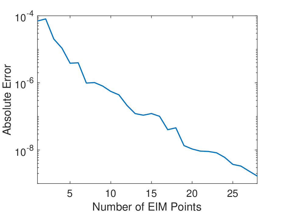
The error plot pictured in Figure 4 shows the error between the EIM approximated solution and the reference solution both evaluated at . This informs our choice of 28 EIM points as we see approximately absolute interpolation error. The location of the 28 EIM points corresponding to the output data, to be matched with the DNN output, is pictured in Figure 5.
4.1.2 Surrogate Quality
In this section we test the quality of the DNN-EIM surrogate. We compare the DNN-EIM solution against the POD and DNN-EIM (s) solutions on the reference solution corresponding to the parameter choice which is not part of the training dataset. Table 2 displays the results. First, we note that DNN-EIM achieves the lowest absolute error and requires the least number of neural network parameters. Second, we can see visually in Figure 6 that the solutions agree to a high accuracy in -norm.
| Methods | No. ResNets | Layers | Width | No. of param. | -error |
|---|---|---|---|---|---|
| POD | 1 | 3 | 28 | 2,492 | |
| DNN-EIM (s) | 1 | 3 | 28 | 2,492 | |
| DNN-EIM | 28 | 3 | 5 | 224 (per ResNet) |


4.2 Kuramoto-Sivashinsky Equation
The Kuramoto-Sivashinsky model is given below with periodic boundary conditions:
| (9a) | ||||
| (9b) | ||||
| (9c) | ||||
We set and use a spectral solver with Crank-Nicolson and Adams-Bashforth (CNAB2) time stepping. The time-step is . The domain is discretized uniformly with meshsize resulting in 1600 spatial degrees of freedom. The reference solution is calculated by setting and .
To generate the training samples for Step 1 of Algorithm 1, we randomly generate 1000 initial conditions of the form with and is sampled from a standard normal distribution with mean zero and standard deviation 1. This will ensure sufficient diversity in the data. We solve (9a) forward in time using these initial conditions and we wait until time units. We collect samples from the solutions every time step at the EIM points 38 times. Since we are learning a one time step solution, therefore we will have 37,000 input-output pairs. The training data will be input output pairs of the form,
| (10) |
Here, (waiting period), is the number of snapshots per solution and is the number of solutions. Next, we proceed with Steps 2-4 of Algorithm 1 and compute the difference between EIM approximation and the reference solution. This is shown in Figure 7. The time integration in (6) is done using 10 time units. We observe the error to be approximately when using 300 EIM interpolation indices or EIM points. This informed our choice to use 300 EIM points for this particular problem.

The ResNets in the neural network surrogate have 8 layers each with a width of 3 neurons.
4.2.1 Neural Network Architecture
In this section, we will cover the structure of our ResNet system. For each EIM interpolation index generated by Step 3 of Algorithm 1, we train one ResNet. The input to the ResNet is the value of our proposed algorithm (solution at the previous time-step) at in addition to the value at neighboring interpolation indices. In one dimension, assume the EIM interpolation indices are ordered according to their position on the real line. Then the input for the ResNet corresponding to the EIM interpolation index is , see Figure 2. The output is the value at advanced in time with time step .
4.2.2 Surrogate Quality
In this section we test the quality of the DNN-EIM surrogate. We propagated forward the initial condition of the reference solution for one time unit or 10 time steps. This is equivalent to 10 neural network evaluations. We then computed the time average relative error between DNN-EIM and the exact solutions over one time unit and obtained a good approximation with absolute error as shown in Figure 8. We repeated the same procedure with a single ResNet with input and output in . This single ResNet has 4 layers with width 300. We observed a time averaged absolute error of .
![[Uncaptioned image]](2305.09842v1/ks_surrogate_err2.png)
This ResNet took approximately 4 days to train while DNN-EIM took one hour using 34 cores. Finally, the DNN-EIM surrogate requires training significantly less parameters as shown in Figure 9.
5 Conclusions
We introduced an empirical interpolation method (EIM) based approach to training DNNs called DNN-EIM. We demonstrated our approach with examples in classification, parameterized and time dependent PDEs. DNN-EIM can be trained in parallel leading to significantly smaller number of parameters to learn, reduced training times, without sacrificing the accuracy. The approach has been applied to standard MNIST dataset, parameterized advection diffusion equation, and space-time Kuramoto-Sivashinsky equation. Future work on this topic includes how to handle more complex cases such as the unsteady Navier–Stokes equations. It will also be interesting to develop a convergence analysis of the proposed algorithm.
References
- [1] H. Antil, T. S. Brown, R. Löhner, F. Togashi, and D. Verma, Deep neural nets with fixed bias configuration, arXiv preprint arXiv:2107.01308, (2021).
- [2] H. Antil, D. Chen, and S. Field, A note on qr-based model reduction: Algorithm, software, and gravitational wave applications, Computing in Science & Engineering, 20 (2018).
- [3] H. Antil, H. C. Elman, A. Onwunta, and D. Verma, Novel deep neural networks for solving bayesian statistical inverse problems, arXiv preprint arXiv:2102.03974, (2021).
- [4] H. Antil, S. Field, F. Herrmann, R. Nochetto, and M. Tiglio, Two-step greedy algorithm for reduced order quadratures, Journal of Scientific Computing, 57 (2013), pp. 604–637, https://doi.org/10.1007/s10915-013-9722-z, http://dx.doi.org/10.1007/s10915-013-9722-z.
- [5] H. Antil, M. Heinkenschloss, and D. C. Sorensen, Application of the discrete empirical interpolation method to reduced order modeling of nonlinear and parametric systems, Reduced order methods for modeling and computational reduction, (2014), pp. 101–136.
- [6] M. Barrault, Y. Maday, N. C. Nguyen, and A. T. Patera, An ‘empirical interpolation’ method: application to efficient reduced-basis discretization of partial differential equations, C. R. Math. Acad. Sci. Paris, 339 (2004), pp. 667–672, https://doi.org/10.1016/j.crma.2004.08.006, http://dx.doi.org.ezproxy.rice.edu/10.1016/j.crma.2004.08.006.
- [7] R. Becker, M. Braack, and B. Vexler, Numerical parameter estimation for chemical models in multidimensional reactive flows, Combustion Theory and Modelling, 8 (2004), p. 661.
- [8] T. S. Brown, H. Antil, R. Löhner, F. Togashi, and D. Verma, Novel dnns for stiff odes with applications to chemically reacting flows, in International Conference on High Performance Computing, Springer, 2021, pp. 23–39.
- [9] S. Chaturantabut and D. C. Sorensen, Nonlinear model reduction via discrete empirical interpolation, SIAM Journal on Scientific Computing, 32 (2010), pp. 2737–2764.
- [10] E. C. Cyr, M. A. Gulian, R. G. Patel, M. Perego, and N. A. Trask, Robust training and initialization of deep neural networks: An adaptive basis viewpoint, in Mathematical and Scientific Machine Learning, PMLR, 2020, pp. 512–536.
- [11] N. Franco, A. Manzoni, and P. Zunino, A deep learning approach to reduced order modelling of parameter dependent partial differential equations, Mathematics of Computation, 92 (2023), pp. 483–524.
- [12] D. Galbally, K. Fidkowski, K. Willcox, and O. Ghattas, Non-linear model reduction for uncertainty quantification in large-scale inverse problems, International journal for numerical methods in engineering, 81 (2010), pp. 1581–1608.
- [13] K. He, X. Zhang, S. Ren, and J. Sun, Deep residual learning for image recognition, in Proceedings of the IEEE conference on computer vision and pattern recognition, 2016, pp. 770–778.
- [14] J. S. Hesthaven, G. Rozza, and B. Stamm, Certified reduced basis methods for parametrized partial differential equations, SpringerBriefs in Mathematics, Springer, Cham; BCAM Basque Center for Applied Mathematics, Bilbao, 2016, https://doi.org/10.1007/978-3-319-22470-1, https://doi.org/10.1007/978-3-319-22470-1. BCAM SpringerBriefs.
- [15] J. S. Hesthaven and S. Ubbiali, Non-intrusive reduced order modeling of nonlinear problems using neural networks, Journal of Computational Physics, 363 (2018), pp. 55–78.
- [16] Y. Maday, N. C. Nguyen, A. T. Patera, and G. S. H. Pau, A general multipurpose interpolation procedure: the magic points, Commun. Pure Appl. Anal., 8 (2009), pp. 383–404, https://doi.org/10.3934/cpaa.2009.8.383, http://dx.doi.org/10.3934/cpaa.2009.8.383.
- [17] R. Maulik, B. Lusch, and P. Balaprakash, Reduced-order modeling of advection-dominated systems with recurrent neural networks and convolutional autoencoders, Physics of Fluids, 33 (2021), p. 037106.
- [18] L. Ruthotto and E. Haber, Deep neural networks motivated by partial differential equations, J. Math. Imaging Vision, (2019), https://doi.org/10.1007/s10851-019-00903-1.
- [19] M. Salvador, L. Dede, and A. Manzoni, Non intrusive reduced order modeling of parametrized pdes by kernel pod and neural networks, Computers & Mathematics with Applications, 104 (2021), pp. 1–13.
- [20] O. San, R. Maulik, and M. Ahmed, An artificial neural network framework for reduced order modeling of transient flows, Communications in Nonlinear Science and Numerical Simulation, 77 (2019), pp. 271–287.
- [21] J. A. Tropp, A. Yurtsever, M. Udell, and V. Cevher, Practical sketching algorithms for low-rank matrix approximation, SIAM J. Matrix Anal. Appl., 38 (2017), pp. 1454–1485, https://doi.org/10.1137/17M1111590, https://doi.org/10.1137/17M1111590.