Symmetry-enriched topological order from partially gauging symmetry-protected topologically ordered states assisted by measurements
Abstract
Symmetry protected topological (SPT) phases exhibit nontrivial short-ranged entanglement protected by symmetry and cannot be adiabatically connected to trivial product states while preserving the symmetry. In contrast, intrinsic topological phases do not need ordinary symmetry to stabilize them and their ground states exhibit long-range entanglement. It is known that for a given symmetry group , the 2D SPT phase protected by is dual to the 2D topological phase exemplified by the twisted quantum double model via gauging the global symmetry . Recently it was realized that such a general gauging map can be implemented by some local unitaries and local measurements when is a finite, solvable group. Here, we review the general approach to gauging a -SPT starting from a fixed-point ground-state wave function and applying a -step gauging procedure. We provide an in-depth analysis of the intermediate states emerging during the N-step gauging and provide tools to measure and identify the emerging symmetry-enriched topological order (SET) of these states. We construct the generic lattice parent Hamiltonians for these intermediate states, and show that they form an entangled superposition of a twisted quantum double (TQD) with an SPT ordered state. Notably, we show that they can be connected to the TQD through a finite-depth, local quantum circuit which does not respect the global symmetry of the SET order. We introduce the so-called symmetry branch line operators and show that they can be used to extract the symmetry fractionalization classes (SFC) and symmetry defectification classes (SDC) of the SET phases with the input data and of the pre-gauged SPT ordered state. We illustrate the procedure of preparing and characterizing the emerging SET ordered states for some Abelian and non-Abelian examples such as dihedral groups and the quaternion group .
I Introduction
Topological order first originated from the study of the fractional quantum Hall effect Tsui et al. 1982; Laughlin 1983. It cannot be described by local order parameters and is beyond Landau’s classification of matter. It exhibits ground-state degeneracy dependent on the topology of the underlying manifold and the excitations, displaying anyonic statistics Wen 1990; Wen and Niu 1990. More recently, it was recognized as possessing some kind of long-range quantum entanglement Chen et al. 2013 and having nonzero topological entanglement Hamma et al. 2005; Kitaev and Preskill 2006; Levin and Wen 2006. In addition to fractional quantum Hall systems and certain spin liquids Balents 2010, there are models that manifest topological order, such as Kitaev’s toric code and quantum double (QD) models Kitaev 2003, their twisted versions Hu et al. 2013, Levin-Wen string-nets Levin and Wen 2005 and more recently fractons Nandkishore and Hermele 2019; Pretko et al. 2020. Topological features that characterize such a phase of matter are robust to local perturbations, which is a property highly desirable in quantum memories Terhal 2015. Some of the topological models also offer the capability of topological quantum computation (TQC) by exploiting the braiding of anyons Kitaev 2003; Nayak et al. 2008; Cui et al. 2015; Mochon 2003, which has emerged as one of the schemes for fault-tolerant quantum computation due to its inherent robustness.
Interestingly, from the perspective of adiabatic connection and quantum circuits, ground states of different phases at zero temperature cannot be connected by either adiabatic evolution or a finite-depth quantum circuits Chen et al. 2010. Intrinsic topologically ordered states therefore cannot be created from a trivial ground state, such as product states, with a quantum circuit of finite depth. When the circuits are required to respect a certain global symmetry, trivial gapped phases can be further fine-grained into distinct classes: those that can be created from product states with symmetric, finite-depth circuits and those that cannot. The latter classes are referred to as nontrivial symmetry-protected topological (SPT) phases Gu and Wen 2009; Pollmann et al. 2010; Chen et al. 2012, and most of them can be classified by cohomology Chen et al. 2013; Else and Nayak 2014.
Quantum technology has been constantly improving and evolving. Several medium-scale quantum computers are available. Recently, certain topologically ordered states, such as those of the toric model, were created by quantum circuits Satzinger et al. 2021, and furthermore, some braiding statistics has also been observed in experiments Banerjee et al. 2018; Kasahara et al. 2018; Andersen et al. 2022; Xu et al. 2022; Iqbal et al. 2023a. Yet, preparation of high-fidelity ground states and precise manipulation of excitations in topological systems still remain challenging in the current era of noisy intermediate-scale quantum (NISQ) devices Preskill 2018.
For the family of the QD models and their twisted versions, i.e., twisted quantum double (TQD) models Hu et al. 2013, there is a well-known correspondence to models of SPT phases Chen et al. 2013; Pérez-García et al. 2008; Jiang and Ran 2017; Williamson et al. 2016a via a procedure called gauging Levin and Gu 2012; Haegeman et al. 2015; Shirley et al. 2019; Kogut 1979. When two quantum states are topologically distinct with respect to a symmetry , then they cannot be transformed to each other with a finite-depth, piecewise local unitary transformation that preserves the symmetry. The classification and characterization of SPT phases with global symmetry in two dimensions is facilitated by a function of , namely a 3-cocycle , which is a representative element of the 3rd cohomology group of , denoted by Chen et al. 2013. At the same time, the TQD model is also characterized by the 3-cocycle: inequivalent choices of the 3-cocycle give rise to distinct intrinsic topological phases Hu et al. 2013. Indeed, the wave function of the TQD model with the gauge group is obtained by gauging the global symmetry in the corresponding SPT wave function. We note that gauging by itself is not a unitary operation; an interesting question is, therefore, whether such a map is physically possible.
It has been known that the ground state of the toric code can be efficiently prepared by measuring half of qubits in a 2D cluster state Raussendorf et al. 2005. The use of measurements thus can provide a route to creating long-range entangled states with finite-depth operations Tantivasadakarn et al. 2021; Piroli et al. 2021; Ashkenazi and Zohar 2022. Ref. Verresen et al. 2021 demonstrated that ground states of QD models with and groups can be prepared through finite-depth local unitary operations supplemented with on-site measurements. It was also argued in Ref. Tantivasadakarn et al. 2021 that a similar procedure should work for QD models with any solvable group , which was later elaborated in Ref. Bravyi et al. 2022 through repeated rounds of finite-depth operations, where each round incorporates unitaries, measurements, feedforward, and corrections. This scheme was further generalized to the general TQD models with solvable groups in Tantivasadakarn et al. 2022a, where the number of measurement rounds was classified for various topological orders, leading to a conjecture of a new hierarchy of topological orders when one includes measurements as an ingredient. It is worth mentioning that further improvement is possible for the QD models with and groups, which can be prepared with a single round of measurements, feedforward, and corrections Tantivasadakarn et al. 2022b. Experimentally, measurement-based gauging is a promising method for realizing nontrivial topological orders in small-scale systems requiring only local unitary operations, mid-circuit measurements, and feedforward corrections Iqbal et al. 2023b; Foss-Feig et al. 2023; Iqbal et al. 2023a.
The present work re-examines the measurement-based gauging from the perspective of group representation theory and provides a characterization of the transformation and emergence of SPT, SET, and intrinsic topological order during gauging. In general, for a solvable group , the corresponding TQD model can be prepared from a -SPT through a multi-step gauging procedure. In this work, we provide two approaches that realize such an -step gauging which reduces to a one-step gauging when is abelian or to a two-step gauging when is dihedral. For non-solvable groups, it is argued that the measurement-assisted gauging procedure cannot be implemented by a finite-depth circuit Tantivasadakarn et al. 2022a.
Interestingly, we find that the intermediate states, that emerge during the multi-step gauging, can be naturally described as symmetry-enriched topological (SET) orders Essin and Hermele 2013; Mesaros and Ran 2013; Lu and Vishwanath 2013; Barkeshli et al. 2019. We also show that, without respecting global symmetry, there is a finite-depth quantum circuit that takes the SET ground state to a ground state of a corresponding twisted quantum double model (TQD).
The essential data of an SET order, besides the intrinsic anyon theory , include the symmetry action as an automorphism on , the symmetry fractionalization class, and the defectification class Barkeshli et al. 2019. A key result of our work is to characterize the resulting SET order given the 3-cocycle that describes the initial SPT wave function. If the emergent SET order has a global symmetry that does not change the anyon type, we develop a general formalism based on symmetry branch line operators for the braiding phases between any abelian anyon in the theory and the anyons obtained from fusing point defects, exactly characterizing the symmetry fractionalization patterns. If the SET order we enter has a global symmetry that does change anyon types, we conjecture the form and algebra of non-abelian symmetry branch line operators that can create the corresponding symmetry defects. Then, by calculating the tensor product of such operators, one can derive the fusion rules of these symmetry defects, which we believe is sufficient to characterize the symmetry fractionalization patterns. We consider the dihedral SPT states as an example to illustrate this case.
The remainder of this paper is organized as follows. In Sec. II, we review the duality between SPT states with global symmetry group and ground states of a twisted quantum double model with a gauge group in two dimensions. This duality is given by a formal gauging map, which turns the global symmetry into a gauge symmetry. In Sec. III, we describe the general procedure of -step gauging -SPT ordered states when is a solvable group in terms of an algorithm (see Algorithm 1 below). In Sec. IV and Sec. V, we discuss 1-step and 2-step gauging respectively, and consider Abelian and dihedral groups as illustrative examples. For the latter, we find that after the first gauging step, the system remains in a SET state where the remaining quotient group describes the global symmetry. Sec. VI contains the discussion on symmetry properties of the emergent SET phases from the perspective of symmetry defects. Using the framework of symmetry branch lines, we relate the transformation of symmetry defects under gauging to properties of the SET phase. We give several examples to illustrate our formalism. In Sec. VII. we make some concluding remarks. The Appendix provides materials that support the results in the main text. For example, we provide a constant-depth unitary circuit to map an SET state to a TQD state in Appendix E. In Appendix J, We also give an alternative gauging prescription based on a different presentation of solvable groups which is alternative but equivalent to the standard one, as proven in Appendix K.
II Fixed-point SPTs, twisted quantum doubles and gauging
On an oriented triangulated lattice , given a finite group , we assign a Hilbert space to each vertex . Then we can write a fixed-point -SPT wave function. To do this, we first assign a group cocycle to each simplex, where is a representative in respecting the cocycle condition,
| (1) |
for any .
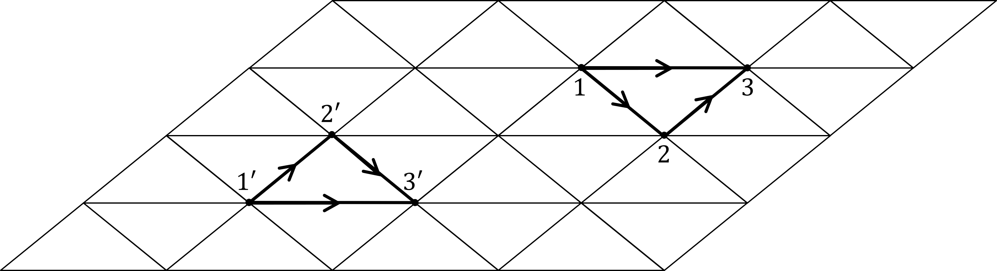
The fixed-point SPT wave function is given by taking a product over all such cocycles,
| (2) |
where indicates the orientation of a simplex (with a given branching structure, and labels the vertices on the simplex), the tensor product runs over all vertices on the lattice, and all the configurations are summed over. Note that we use a convention from Ref. Williamson et al. 2016b, which is slightly different from Ref. Chen et al. 2013, for the sake of convenience in later discussions. This state can be obtained by the action of a unitary operator on the product state ,
| (3) |
We define the left/right action of on as
| (4) |
Then the global symmetry action (in our convention) on SPT state yields
| (5) | ||||
where in the second line we used a change of variables and we have defined a phase factor in the fourth line.
Suppose is the two-dimensional spatial manifold on which the Hilbert space is defined, and is an interval in the (Euclidean) time direction. The manifold is now three-dimensional. We triangulate the by 3-simplexes (tetrahedrons) with the constraint that each time slice at and matches the original two-dimensional lattice; see Fig. 2. The amplitude Amp is computed once the triangulation of is specified. We now give more details.

We assign a 3-cocycle to each tetrahedron as in Fig. 3. The phase factor can be seen to be Chen et al. 2013
| (6) |

When the spatial manifold is closed, using cocycle conditions, one can show that . Therefore, the SPT state is invariant under the global symmetry transformation,
| (7) |
Due to this symmetry, this state can be written schematically as (where we have suppressed the indices in for simplicity),
| (8) |
where denotes the product of cocycles, and and are vertices connected by an edge, .
II.1 Gauging global symmetry

Under a gauging map as shown in Fig. 4, the vertex degrees of freedom (DOFs) are mapped to the edge DOFs,
| (9) |
This in turn maps the SPT state to an intrinsic topologically ordered state Yoshida 2017
| (10) |
which is a ground state of the twisted quantum double (i.e., described by the Dijkgraaf-Witten theory) Dijkgraaf and Witten 1990. The twisted quantum double can be formulated on a triangulated lattice with a Kitaev’s Quantum Double-like Hamiltonian Hu et al. 2013,
| (11) |
where and stand for the vertices and plaquettes, respectively, on the lattice. The vertex operator
| (12) |
is hermitian and is a projector (see appendix A), where and are left and right action of the group element on the edge . When emanates from the vertex to another vertex, we apply in Eq. (12), When flows to the vertex , we apply .


The phase is a product of the cocycles corresponding to the tetrahedrons with appropriate orientations in the prism in Fig. 5, where the correspondence between a tetrahedron and a 3-cocycle is established in Fig. 6. Furthermore, this phase factor is the commutator between the right action of on vertex and the unitary operator introduced in Eq. (3),
| (13) |
where we use () when the edge ends at (emanates from) vertex .
The plaquette operator is
| (14) |
where is the Kronecker delta function. The resultant state from the gauging map is the ground state of this Hamiltonian,
| (15) |
The local excitations of TQD model are fractional charges called anyons, which can be classified by a unitary modular tensor category (UMTC); see, e.g., Lin et al. 2021. One thing to remark is that the convention here is slightly different from the one used in Yoshida 2017 and Hu et al. 2013 for the sake of convenience in later discussions.
II.2 Gauging a subgroup of
One can introduce a gauging map that corresponds to gauging only a normal subgroup of . We have the quotient group with an embedding
| (16) |
Any element has a unique decomposition , where and . Under the map, the normal part of vertex DOFs are mapped to edge DOFs, as illustrated in Fig. 7,
| (17) |

This maps the SPT state to
| (18) |
One point to notice is that the above state has a global symmetry under action , where is the right action of on all vertices (e.g., ) and is the conjugation by on all edges defined as
| (19) |
The second point is that the state is a ground state of a Kitaev’s Quantum Double-like Hamiltonian,
| (20) |
where and stand for the vertices and plaquettes on the lattice.
The vertex operator is
| (21) |
The phase is the product of the cocycles corresponding to the tetrahedrons with appropriate orientations of the prism in Fig. 8, where the correspondence between tetrahedron and 3-cocycle is established in Fig. 9.

The plaquette operator is simply the following,
| (22) |
Suppose , we label the embedding of in as , where . The additional vertex operator is
| (23) |
We can always apply a finite-depth local unitary to bring all the vertex DOFs to the identity element (see appendix E) such that the state becomes
| (24) |
This is a TQD state with the 3-cocycle being the restriction of on subgroup . Thus we obtain the anyons and their braiding, which is the same as in . Furthermore, the state is essentially a ground state in an SET phase with the global -symmetry.
II.3 Classification of SETs
Here we briefly review some terminology relevant to SET phases for the convenience of later discussions. This section will be based on Refs. Barkeshli et al. 2019; Chen 2017. In general, assuming the symmetry preserves locality, an SET phase is determined by its anyon set (UMTC) , its -symmetry action as an automorphism on , symmetry fractionalization class (SFC) and symmetry defectification class (SDC) Barkeshli et al. 2019. We first assume the symmetry actions are unitary and always give the trivial automorphism on , i.e., the symmetry does not change anyon types. Consider a state with anyons present sufficiently far away from each other on a sphere. Therefore, the anyons should be able to fuse into the vacuum charge. The symmetry operators respect the multiplication rules . Under our assumptions, the symmetry operator can be decomposed as some local unitaries , near the anyons,
| (25) |
Each local symmetry action can be projective,
| (26) |
where the phase only depends on anyon type and satisfy
| (27) |
whenever the multiplicity is . It is proved in Ref. Barkeshli et al. 2019 that a phase with the above properties is related to the braiding phase between anyon and some other abelian anyon in the theory,
| (28) |
We note that one can redefine the local unitary by an arbitrary phase factor ,
| (29) |
where satisfies
| (30) |
whenever the multiplicity is . Again, the phase factor can be written as a braiding phase between anyon and an abelian anyon , i.e., . The abelian anyon after the redefinition will be
| (31) |
Further, according to the associativity condition , we have
| (32) |
To conclude, the distinctive patterns of symmetry fractionalization are characterized by the class in cohomology group , where is the group formed by abelian anyons via fusion algebra Chen 2017.
Another way to see the symmetry fractionalization classes is to construct a -graded category from the anyon theory including the point defects
| (33) |
where and denotes the identity element in . A distinctive -graded category is a candidate for an SET order. According to Ref. Barkeshli et al. 2019, when the symmetry does not change anyon types, one can always choose an abelian defect from each sector and label it as . The fusion of defects respects the group multiplication structure,
| (34) |
for some abelian anyon . Furthermore,
| (35) |
This abelian anyon is exactly what we have defined above for projective phase . The class is in the cohomology group , which classifies the SFC.
In generic cases, when the symmetry does change anyon types as an automorphism of ,
| (36) |
it turns out that not every sector has an abelian object. Therefore, we cannot write the fusion rule as in Eq. (35).
The fusion rule of a -graded category can be written as
| (37) |
Consequently, each element specifies a potential way of modifying (the SET order) via
| (38) |
Therefore, in generic cases, the potential symmetry fractionalization classes are elements of an torsor. In this work, we will not analyze the SDC in detail, and we simply note that one can enter a different SDC by stacking a -SPT state onto the SET state. In our framework, after gauging the normal subgroup, a global -transformation will locally serve as an automorphism of , mapping an anyon with flux to an anyon with flux . Later in this work, we will analyze the phases of some SETs in which the automorphism on is either trivial or nontrivial.
III -step gauging of 2D SPT via measurement
(b) -SPT fixed point state (defined in Eq. 8) on a lattice with vertices and edges .
(c) as defined in Eq. 41
(d) Generalized Pauli operators as defined in Eqs. 42 and 43 acting on the abelian subspace defined by an embedding of in .
In this section, we present the procedure to gauge a -SPT state of a group that can be factorized into abelian groups with steps. (We note in this section, refers to the number of steps rather than a normal subgroup. But it should be clear from the context.) A similar method was proposed by Tantivasadakarn et al. 2022a and Bravyi et al. 2022. In Tantivasadakarn et al. 2022a, the authors considered the solvable group and its derived series which consists of normal subgroups which are commutator subgroups of the previous group in the series. They proposed a gauging procedure for a particular sequence of normal subgroups. In Bravyi et al. 2022, on the other hand, they proposed to implement the gauging procedure for a solvable group inductively, i.e., implement the gauging of a cyclic group, assuming the remaining quotient group is already gauged. In our procedure, we do not restrict ourselves to a particular derived series for the solvable group. This in turn helps us to prepare different types of SETs. We give the steps for gauging a -SPT state explicitly.
Before presenting the gauging procedure in Algorithm 1, let us go through the most relevant definitions first. A group is a solvable group if there are subgroups such that is normal in , and is abelian for . Given the embedding map from each into , every element can be written as
| (39) |
where . Similarly, for another group element , we have the decomposition . Under this convention, we write down the multiplication between and as
| (40) |
Now, let us define the relevant unitaries and measured observables that will be used in the gauging procedure. We typically consider a state defined on a lattice with vertices and edges where the local Hilbert space depends on the group and is labeled by its group elements . Given an embedding of into as described above, we can define for all the following unitary controlled on vertices and targeting the shared edge:
| (41) | ||||
where . This unitary will be used to entangle vertex DOFs with edge DOFs
Measurements of abelian subgroups will play an important role in the gauging procedure which is why we will now introduce the generalized Pauli-observables for an abelian group . (We note that it should be clear from context whether the symbol represents a group or a Pauli operator.) Any element can be written as where . Given this representation, we write the local Hilbert space basis as . This allows us to define the following generalized local Pauli operators by their action on this basis:
| (42) | ||||
| (43) |
where indicates addition modulo and is the -th root of unity . Importantly, this allows us to define a Fourier-transformed basis as follows,
| (44) |
where .
Note that in Algorithm 1, the local Hilbert space dimension is given by the non-abelian group , so we understand all the above unitaries and bases as defined on an embedded subspace given by . See the discussion above Eq. (39).
We will now use the above equations to implement an -step gauging procedure. We will gauge the -symmetry of the state defined on the vertices of a lattice sequentially in steps. We present the procedure in Algorithm 1 and consider the details below:
- (1)
Include ancillas. Add ancillas in the state , where is the identity element, on the edges between the vertices.
- (2)
Entangle gauge and matter DOFs. Apply the following 2-controlled-shift operators with controls on neighboring vertices (oriented as ) and the target on the in-between ancilla:
(45) Here we have used to denote the part of the decomposition which lies in ; that is, for with , .
- (3)
Measure on matter DOFs. After measurement of the quotient part on each vertex (i.e., in the bases defined in ), with the outcome being on a vertex ( being -th root of unity), there is a corresponding phase factor from the wave function overlap in step (3) of Algorithm 1. These phase factors can be seen as some abelian chargeons on vertices. See an example in Eq. (IV).
- (4)
Correct phase factors. The phase factors arising from step (3) can be corrected as they can be expressed as a product of phase operators acting on the edge DOFs (see e.g., Fig. 10). Therefore, we can apply counter -operators on a set of edges , i.e., , where the exact form of can be deduced from the measurement outcomes. For example, we can move the phase factors on a vertex by performing operators on its neighboring edge and by doing this repeatedly we can move all the phase factors to one single vertex (via the transmutation rule, see, e.g. Fig. 10), therefore annihilating them altogether, due to the symmetry constraint (see Eq. IV and the discussion below it). The set of such edges is an example of , but it is not necessarily optimized. (See also the following two sections for concrete examples.) After measurement and correction, the vertex DOF is mapped from to , where and . The resultant state is a -SET ground state.
- (5)
Repeat the procedure of entangling gauge DOFs on edges and matter DOFs on vertices. Apply the following unitary similar to before:
(46) - (6)
Measure on the matter DOFs and correct the corresponding phase factors from the measurement. This results in a -SET ground state.
- (7)
Repeat this process for all except the last quotient group .
- (8)
At the last step, apply the gauging and measurement procedure for . Specifically, first apply
(47) measure , and then correct the corresponding phase factors. This gives us a -TQD state.
It is worth remarking that in the expressions above, we always use the multiplication rules of the entire group . For instance, if we take , their product is not necessarily in (it is in only when the extension is central). This seemingly makes the remaining global symmetry algebra non-closed, i.e., would produce components in the subgroup (recall that for some ). Nonetheless, instead of in the above step (4), we have , which can absorb the potential components, making the multiplication closed. We can therefore define the global symmetry group of SET as such. Moreover, the state after applying is symmetric with . It also follows that the phase operators resulting from the measurement of can be corrected as the global symmetry gives a constraint on measurement outcomes, which will be discussed later.
In the following, we will consider the 1-step gauging for abelian groups in Sec. IV to illustrate correction processes. Then we will consider the 2-step gauging for dihedral groups in Sec. V. The two-step and multi-step gauging can be also applied to abelian groups as well, and in the intermediate steps, SET states can emerge. We will discuss the phase of such SET states in Sec. V. Then in Sec. VI, we introduce the framework of the symmetry defect branch line and discuss the SET phases for several more examples.
We give an alternative procedure for the -step gauging in Appendix J. This gauging procedure is implemented for a group which admits sequential normal subgroups (see Appendix J for definition). This criterion is in fact equivalent to the group being solvable (see Appendix K for a proof). The two procedures differ in the way in which the product of group elements are written down (compare Eq. (40) and Eq. (282)). Apart from that, in the procedure given in this section, we gauge the quotient groups in every step, while in the procedure given in Appendix J we gauge normal subgroups in each step. As mentioned earlier, in Ref. Tantivasadakarn et al. 2022a, the commutator subgroups of the previous group in the series of a solvable group are gauged successively.
IV 1-step gauging: Abelian groups
In this section, we review the gauging procedure for abelian groups Tantivasadakarn et al. 2021; Tantivasadakarn et al. 2022a. We start with the SPT state given in Eq. (8). The gauging map can be implemented by first transferring the corresponding group elements to edges and then by measuring the vertices, where our state is projected to a quantum double state with (unwanted) charges whose configuration is given by the measurement outcomes. The excitation due to the randomness of measurement is then corrected by a certain finite-depth procedure. The steps are described in more detail as follows:
- (0)
Prepare the SPT state on vertices. We use local control-phase gates to prepare the SPT state from a direct product state.
- (1)
Include ancillas. Add ancillas in the state , where is the identity element, on edges between adjacent vertices. The ancillas become the gauge DOFs
- (2)
Entangle gauge and matter DOFs Apply the following controlled-controlled-shift operators with controls on the neighboring vertices of an edge (oriented as ) and the target being the ancilla on the edge between the two controls:
(48) At this point, the (pre-measurement) state is
(49) - (3)
Choose a measurement basis in the algebra, then project the matter DOFs onto the basis via measurement. A natural basis can be chosen if we order elements in as an ordered list , where , . (Note that the subscript in here denotes the labeling of the group elements of , not the vertex.) Then we simply use the Fourier basis to perform measurements on vertex DOFs, where we have defined . When , we project the matter DOFs onto this basis via measuring the generalized (qudit) operator.
- (4)
Correct excitations in the twisted quantum double. The correction can be done with a finite-depth circuit.
We give more explanation on the procedure for the case with below. For the group, the wave function can be written using the qudit system. The basis vector () and the generalized Pauli operators satisfy
| (50) |
with , which is much simpler than the general abelianized basis in Eqs. (42) and (43). Starting from a SPT on a triangulated lattice, we first add ancillas to all the edges in a product state with . Then we apply the controlled gate in Eq. (48), which is a set of controlled- gates. Then the gauge DOFs are as given by the gauging map in Fig. 4. The next step is to disentangle matter DOFs by measuring the operator on all vertices. After measurements, the matter DOF at a vertex is projected onto , where , and . Suppose the measurement outcome on the vertex is . We write the basis associated with measurement outcomes as
| (51) |
Then the total wave function after measurements (with the gauge part being projected to ) is written as
| (52) |
where and is the phase factor inherited from the SPT state (i.e., a product of 3-cocycles). Note that is the edge ; many edges can share a vertex but the factor only appears once. Due to measurement, the vertex DOFs have been disentangled from the edge DOFs, and the edge DOFs form a state that is a ground state of the twisted quantum double in the flux-free sector up to a factor , which can be interpreted as an chargeon on the vertex .
In what follows, we describe how to remove the excitations in . First, the set of measurement outcomes is restricted to , with being mod , due to the global symmetry of the SPT state. The global symmetry implies
| (53) |
so it should be satisfied that
| (54) |
which gives the constraint , meaning .
Next, the measurement with gives us a phase when contracted with the basis . Due to the constraint , one can always find a set of paths such that we can rewrite the phase factor as , or equivalently , in terms of the phase operator supported on the paths. Concretely, we use a type of relations, which we call the transmutation rules, illustrated in Fig. 10. For , the relation is
| (55) |
We apply the phase operator on the paths to remove the chargeons. Given that these operators commute, they can be applied all at once. Hence, our gauging procedure assisted by measurement requires only finite time steps or a finite-depth quantum circuit (with intermediate measurements).

Let us give two remarks here. The reason that we can correct the state by moving all factors to one vertex is because of the fact that all chargeons in are abelian anyons. This procedure can be straightforwardly generalized to group, where we measure , , …, etc. on all vertices after we entangle gauge and matter DOFs. This occurred previously in the general -step gauging in Sec. III. However, to explain the detailed correction there would incur cumbersome notations. The example of in this section should now make the procedure clearer. Different measurement outcomes will give rise to different chargeons in the flux-free sector, which are all abelian anyons. (Note that we do not have fluxons, as we began with a flat-flux configuration followed by the controlled-controlled operation that does not create fluxons.) Therefore, the state after measurement is still correctable within finite steps.
V 2-step gauging: Dihedral group and intermediate SET states
When we attempt to gauge nonabelian SPT states using measurement, although one can always choose a suitable basis such that the factors are correctable, one crucial problem is that the phase factors that arise from measurement do not necessarily correspond to abelian anyons as in the case above; this makes correction with a finite depth circuit a nontrivial problem. In Ref. Verresen et al. 2021; Bravyi et al. 2022, there were two different ways proposed to prepare the ground state of the quantum double model. In Ref. Bravyi et al. 2022, a toric code ground state is prepared first, and it is coupled to the product state using controlled gates. Then the part is gauged via the measurement-assisted one-step gauging in Ref. Tantivasadakarn et al. 2021.
We will show in this section that, for the symmetry group being the extension of two abelian groups, by choosing some abelianized basis, we can still perform a 2-step gauging procedure on -SPT states via measurement. In the case with , our procedure would be equivalent to first preparing the -TQD ground state, and then coupling to the -SPT state using entangling gates and controlled gates. The correction process for the 2-step gauging is still fairly simple, i.e., via finite-depth quantum circuits. The complete procedure to gauge the abelian -symmetry (i.e., the normal subgroup) of a -SPT state and then to gauge the quotient -symmetry of an SET is as follows:
- (1)
Include ancillas. Add ancillas in the state , where is the identity element, on edges between adjacent vertices. The ancillas will become the gauge DOFs
- (2)
Entangle gauge and matter DOFs. Apply the following controlled-controlled-shift operators with controls on neighboring vertices (oriented as ) and the target on the ancilla on the in-between edge :
(56) The purpose of this step is to mimic the gauging map in Eq. (17).
- (3 & 4)
Measure on matter DOFs and correct the factors. After measurement, with the outcome being , there is a corresponding phase factor . Using the transmutation rule for , one can correct all those factors by moving them to one single vertex, resulting in an SET ground state.
- (5)
Further entangling the quotient part of the gauge and matter DOFs. We apply a controlled-conjugate operator with the target being the ancilla (oriented as ), and the control being :
(57) where denotes the quotient part of via an embedding in Eq. (16). Notice that the normal part of the matter DOF has been wiped out by measuring , while the quotient part still remains, which makes the above controlled-gates possible to implement. The edge DOFs are now .
- (6 & 7)
Measure on matter DOFs, and correct factors. Their correction is straightforward; we apply operators on edges to move all ’s to one vertex.
In the following, we will apply the above procedure to several cases.
V.1 Gauging SPT
The group is . Any element can be written as , where , . We define the decomposition of a group element respectively as
| (58) | ||||
| (59) |
with the former being the normal part (), and the latter being the quotient part () of . We then define the shift operator in each part as
| (60) | ||||
The phase operators, which are known as the clock operators, in each respective part, are
| (61) | ||||
where . The gauging step (2) transforms the ancilla DOF on edge from identity to .
Then in step (3) we measure on all the vertex DOFs. Suppose the measurement outcome is on vertex (where ). The state after the measurement is projected into
| (62) | ||||
The phase factor depends on the measurement outcomes . In order to correct them, we employ the transmutation rules for factors
| (63) |
As in the case with in the previous section, we have due to the -symmetry. By inserting corresponding numbers of operators on the edges, we can move the factors on vertices around and cancel them altogether. Equivalently, one can simultaneously apply operators supported on strings whose endpoints correspond to nontrivial measurement outcomes. This gives us the state
| (64) | ||||

After the gauging step (5), the edge DOFs are conjugated and shifted by , giving rise to
| (65) | ||||
Step (6) is similar to step (3). By measurements, the state is projected to
| (66) | ||||
where we have assumed that from the measurement on vertex (where ). In order to correct the phase factor , we employ the transmutation rules for factors:
| (67) |
which is illustrated in Fig. 12. This rule, just as the rule for in step (4), allows us to move all the factors to a single vertex and annihilate them. This is guaranteed by the -global symmetry in (see Appendix C),
| (68) |
which implies that the measurement outcomes satisfy in this case, as the global symmetry is . After we apply the corresponding correcting phase factors to edges, we thus obtain a -TQD ground state.

V.2 SET with Symmetry
Let us begin by recalling that the gauging map in Eq. (17) gauges the normal subgroup of . In our procedure, after we correct the factors in step (3), the state is essentially a ground state of the SET phase. In what follows, we first look into the entanglement structure of the wave function after gauging the normal subgroup . Then we identify the class of this SET phase, namely, the unitary modular tensor category (UMTC) that contains all anyonic excitations, the symmetry action as an automorphism of , the symmetry fractionalization class and defectification class Barkeshli et al. 2019.
We write the element in as with some slight abuse of the notation, where and . It should be clear from the context when is a number or a group. A representative of the cocycle in is
| (69) | ||||
where , and . As pointed out in Sec. II, the anyon set (UMTC) is determined by the restriction of on subgroup (i.e., setting ),
| (70) |
Different values of are in one-to-one correspondence with different twisted quantum double phases . An anyon in these phases is characterized by its flux , and a projective representation of , satisfying
| (71) |
which means , where is an ordinary representation of .
Using Lyndon–Hochschild–Serre spectral sequence Lyndon 1948; Hochschild and Serre 1953; Chen et al. 2012, we can decompose the cohomology class of the group as
| (72) |
This suggests that this SET state is composed of a TQD and a -SPT state. A natural question is whether the wave function of the whole system is decomposed into a product of the two corresponding parts.
It turns out that we can write the 3-cocycle in Eq. (69) as
| (73) |

where the phase is defined from the 3-cocycle of ,
| (74) | ||||
and is a representative in . Every plaquette on the spatial manifold is associated with such a phase. The product of them over all plaquettes gives
| (75) |
The sum of the above phase over all possible configurations gives the wave function of a ground state of .
The phase is defined from the 3-cocycle of , ,
| (76) |
The product of this type of phases gives
| (77) |
The sum of the above phases over all possible configurations results in the wave function of a -SPT state. The part in Eq. (73) is
| (78) |
which is nontrivial when . Similarly, we define the product of this type of phases over the spatial manifold as ,
| (79) |
Thus the resulting state after gauging from an -SPT state is
| (80) | ||||
which is an entangled state between a -TQD ground state and a -SPT state. When , we have , hence the wave function of the system becomes
| (81) | ||||
which is a product state of a Toric code ground state and a -SPT state.
Having obtained the SET wave functions, we now discuss the effect of the global symmetry action. The symmetry action in the -SPT state is mapped to , under which an anyon with flux will be mapped to one with flux . And a chargeon will be mapped to its antiparticle under the symmetry. According to Sec. II.3, the possible SFC will be given by elements in a torsor. With different values of , the abelian group could be either or . In either cases, the cohomology group turns out to be trivial, and so is its torsor. Therefore, the TQD has only one possible symmetry fractionalization pattern. Moreover, different values of in the 3-cocycle of result in different symmetry defectification classes (SDC) in the SETs, which are obtained by gauging the normal group. This is expected because as seen from Eq. (80), different values represent different -SPT states entangled with some -TQD state.
Let us remark that this construction for has a natural generalization on groups, where one first gauge , resulting in an SET on which the symmetry acts to conjugate the gauge DOFs. Different parent SPT phases will result in different anyon theories and different SDCs, but always some unique symmetry fractionalization pattern. One can further gauge the quotient symmetry to obtain TQD.
V.3 Gauging SPT
Now we discuss the process of 2-step gauging a generic SPT state via measurement under a similar type of abelianized basis. As in , an element in group can be written as
| (82) |
We will thus use a generalized definition of operators as for in Eqs. (58), (59), (60), and (61).
After applying the control gate to set the DOFs on edges, e.g., , to , measuring on vertices, and correcting all chargeon excitations, the resultant state is a ground state in a -SET phase with a global symmetry at this intermediate stage. According to the multiplication rule of , just as in , the symmetry transformation conjugates all the gauge DOFs.
As an illustration, we will consider the group. Using the Lyndon-Hochschild-Serre sequence, the cohomology group can be decomposed as
| (83) | ||||
Again, the cocycle factorizes as
| (84) |
where and are defined similarly as for the group in the last section, while and depend on both quotient and normal parts of the vertex DOFs. From this decomposition, it is clear that after gauging the normal , we have an entangled state between the -TQD state and the -SPT state. Because of the additional entanglement via , we expect to have a nontrivial SFC from gauging the symmetry of a -SPT state.
Indeed, in the next section, we will show that the current 2-step gauging setup could result in different SFCs. To do so, we first introduce symmetry branch line operators and other necessary tools to determine the SFC. We will also discuss several examples, including the above -SET phase.
VI Symmetry Defect in SPT and SET
In this section, we will apply the notion of symmetry branch lines introduced in Ref. Barkeshli et al. 2019 and formulate corresponding symmetry branch line operators in SPT phases, as well as their relation to ribbon operators in TQD. We then show the gauging procedure transforms such operators in SPT phases into symmetry branch lines in SET phases and discuss how their fusions relate to the symmetry fractionalization classes (SFC) in a few examples.
VI.1 Symmetry Branch Lines
To introduce symmetry branch lines, we start with the symmetry action in an SPT wave function. We recall in Eq. (2) the SPT wave function on a triangulated spatial manifold,
| (85) |
When the manifold is closed, the global symmetry action leaves the entire SPT state invariant. We can also consider the symmetry action on a sub-manifold Else and Nayak 2014, such as the one shown in Fig. 15(a),
| (86) |
Triangulating the frustum created by lifting vertices in , we have multiple tetrahedrons. We associate each tetrahedron in the frustum as in Fig. 15(a) to a 3-cocycle, such as the one in Fig 3, to which we assign a phase factor . The product of all such cocycles composes the factor , namely,
| (87) |
Using the cocycle conditions, it turns out that only depends the DOFs around and does not depend on those DOFs deep inside , see Fig. 15(b), and its expression is
| (88) |
where the extra factor to the product on the r.h.s. is
| (89) |
when contains vertices equipped with the branching structure, , see Appendix D. In fact, one can introduce an operator that is supported only on such that Else and Nayak 2014
| (90) |

To do this carefully, we need to first introduce a pre-gauge structure Dolev et al. 2022. Namely, we introduce a -DOF on every edge (which we will be set to the identity group element to begin with). One can think of the edge DOFs as the discrete gauge field. After introducing such a gauge field, one may write the local symmetry action on both vertex and the surrounding edges . This is also called the “gauge transformation” operator on a vertex as
| (91) |
where denotes those edges with one end being and where is the left (right) actions of on , when the edge flows to (emanates from) . Furthermore, the “interactions” should also be written in a gauge invariant way. Namely, instead of the original SPT Hamiltonian, one can write the gauge invariant version as follows,
| (92) |
where the phase was previously introduced in Sec. II.
Taking any ground state of this Hamiltonian, we can impose the gauging map in the presence of the pre-gauge structure,
| (93) |
under which, the state would be mapped to a ground state of the TQD model. One special ground state of this Hamiltonian would be
| (94) |
where we have taken the original SPT state, which has on all edges. One can easily verify that is still a ground state, for any vertex on lattice and . We define the gauge transformation over a region as . If the spatial lattice is closed, we write and one can check that
| (95) |
Therefore, the operator mimics the behavior of global symmetry operator after introducing the pre-gauge structure.
Now we introduce the definition of symmetry branch line operators on states with trivial edges ,
| (96) |
but unlike , the operator only takes effect on . We find that the following expression of ,
| (97) |
where is a reference vertex on as shown in Fig. 15(b). The phase is the product of cocycles associated to the tetrahedrons in Fig. 15(b), with ,
| (98) |
The operator is a product of shift operators on the edges crossed by . In general, with on a ribbon is defined as follows,
| (99) |
This operation can be regarded as the non-onsite symmetry action on the boundary , and its definition can be extended to the case whenever there is no flux in the state (i.e., for every plaquette, .). From direct calculation using Eq.(96) and the fact that , one can easily show that the multiplication rule of ,
| (100) |
is exactly the multiplication rule of the group , as expected for the symmetry branch lines. One can also show the multiplication rule of directly using the form in Eq. (97), see Appendix D. Indeed, if we use the operator
| (101) |
to project any ground state onto the gauge invariant sector, we would also have a TQD ground state. The operator above in Eq. (101) can be seen as a superposition of different meshes of symmetry branch lines.


There are two important remarks here. The first is that inserting a symmetry branch line on an SPT state is to create a point symmetry defect , move it along and annihilate it with . The multiplication rule above indicates that the fusion between point defects is . Second, we can consider the global symmetry action on the state with a branch line on , i.e., . It turns out that
| (102) | ||||
where . In other words, the global symmetry transformation on is .
VI.2 More on Symmetry Branch Lines
To discuss further the symmetry branch lines, we first remind the readers of some definitions in group cohomology. Given a 3-cocycle as a representative of element in , the slant product is defined as Propitius 1995
| (103) |
which is naturally a conjugated 2-cocycle, i.e., a representative in . Namely, it satisfies the following condition,
| (104) |
When is a representative of the trivial element in , there exists a conjugated 1-cochain , such that
| (105) |
There is another product that will also become useful later:
| (106) |
which, however, is not a 2-cocycle nor a conjugated one.
For a general state with a nontrivial pre-gauge structure, we give a conjecture for the expression of symmetry branch lines. We can follow the similar idea as in the previous section to introduce the branch line operator from the symmetry action in the region , when all the plaquettes on are fluxless (i.e. ), and the flux on each plaquette () is in the centralizer group , see Appendix D for details. If we start from vertex and go along , the holonomy, i.e., the product of group elements on all the edges along the path, is , and the resulting symmetry branch line is
| (107) |
with the operator on the r.h.s. being
| (108) |
where is a 1-cochain defined in Eq. (105), and is a reference vertex. The phase is the product of cocycles associated to the tetrahedrons in Fig. 15(b), with and , namely,
| (109) |
The operator is defined in Eq. (229), and is defined as follows.
| (110) |
In order to make well-defined, we require that and commute. For an SPT state, we have that , and this is trivially satisfied. With the above discussions, we can derive the multiplication of branch line operators (see Appendix D for the proof),
| (111) |
We also note that given a 3-cocycle , the phase factor is not unique. One can always replace by , where satisfies . This corresponds to a different choice of in , and we will illustrate this with concrete examples below.
We recall the gauging map in the presence of the pre-gauge structure,
| (112) |
Under this, the operator is mapped to
| (113) |
Notice that after gauging, the dependence of the operator is summed over as in the sum of above. Therefore, the resultant operator under the gauging map does not depend on any reference vertex.
In the case when , we can choose , then the operator is reduced to the trace of the ribbon operator that creates an -fluxed anyon in the quantum double (see, e.g., Ref. Bombin and Martin-Delgado 2008),
| (114) |
where on the left-hand side, is the conjugacy class of , is the trivial representation of the centralizer group . In order to construct the operators , one enumerates the elements of the conjugacy class as , together with a suitable subset such that . The operator on the left-hand side is a ribbon operator labeled by topological charges, and on the right-hand side is a ribbon operator in a basis labeled by group elements.
For a generic 3-cocycle , when is in the center of , the -fluxed anyon is abelian. Then we have the following relation via the map ,
| (115) |
where is a ribbon operator defined in TQD for abelian groups in Ref. Mesaros and Ran 2013.
The algebra of ribbon operators can be inferred from the quasi-Hopf algebra Propitius 1995; Dijkgraaf et al. 1991. To be more concrete, suppose we insert an -flux on ribbon . Operator thus satisfies the multiplication rule
| (116) |
which is consistent with our result of the branch line multiplication in Eq. (111), since we expect the gauging map to preserve the operator algebra, which is quasi-Hopf in this case.
One thing to notice is that, in order to write down , we have assumed the existence of . This is not always possible. When such does not exist, even when is in the center of , the -fluxed anyon can still be nonabelian Propitius 1995. For example, if is a type-3 cocycle of , the anyons in the TQD are generally nonabelian. Therefore, one could not expect to write down ribbon operators as we have defined above. However, when we gauge one of the groups from the SPT, we would enter an SET order with global symmetry . It turns out that we can try to write the branch line operators in the SET order, and from the algebra of which, one can infer the symmetry fractionalization patterns. We will leave this for further discussion later in this paper.
Throughout this paper, we have mostly used branch lines on closed curves. As we have seen earlier, for closed branch line operators, we need to specify a reference vertex . Imagine if we could define branch line operators on an open ribbon that starts from vertex and ends at vertex , we have two natural reference vertices. In the case when is abelian, the gauging map will take such operators to ribbon operators defined in Cheng et al. 2017. If we assume that the multiplication rule stays the same, then we have
| (117) |
where the factor
| (118) |
is the only object that is ‘pumped’ out when we apply the anomalous non-onsite transformation and its inverse accordingly. One can check from the cocycle condition (see also Ref. Dijkgraaf et al. 1991) that
| (119) |
showing that satisfies the ‘twisted’ cocycle condition. One can thus use this to write
| (120) |
If is one of the endpoints of the defect operators, then we essentially pump a factor to the state. The phase factor is a conjugated 1-cocycle, i.e., , where labels conjugacy classes of , and is the corresponding centralizer group. We will call this factor the SPT pumping factor, since, by fusing defect operators, we pump a lower dimensional SPT state (in this case a d SPT state) on the boundary of the line after the application of . This is a generalization of a previous abelian case analyzed in Ref. Wen and Potter 2022. If is abelian, for every element , the factor is a 1d representation of group , i.e., one pumps a 0d -SPT state on the endpoints of an open ribbon.

VI.3 Symmetry Branch Lines in SET Phase
As discussed in previous sections, we can gauge a normal subgroup of . Then we enter an SET phase with global symmetry . Any group element in can be decomposed as . The SET wave function is
| (121) |
When the group element commutes with all the elements in the normal subgroup, a branch line operator we introduced for the -SPT state will be mapped to another operator under the gauging map . Further, the operators defined as such respect the same multiplication rules as do. Denoting , the operator is written as
| (122) | ||||
| (123) |
When , the operator is a ribbon operator creating a gauge flux in the SET. When , i.e., for some element , the operator creates a flux that corresponds to an element in the global symmetry group and thus is a branch line operator. The multiplication rule of such operators is
| (124) |
which, in turn, leads to
| (125) |
where the phase factor on the r.h.s. is
| (126) |
When we take two branch line operators and , i.e., both , and multiply them together, then the resulting is not necessarily a branch line operator, because is not always trivial. As we will see in more details later, this indicates a nontrivial symmetry fractionalization class (SFC) of the SET order.
We can always apply a finite-depth local unitary to take all the vertex DOFs to the identity element (see appendix E), such that the state becomes
| (127) |
This is a TQD with the 3-cocycle being the restriction of on subgroup . An abelian anyon in this model is determined by its flux (i.e., conjugacy class ) and charge (i.e., a conjugated 1-cochain such that , i.e., ). The symmetry action on the anyons are given by
| (128) | ||||
| (129) |
From our previous analysis, we know that the automorphism maps -fluxed anyon to -fluxed anyon, thus we have Eq. (128). Furthermore, the automorphism will map a chargeon (i.e., a representation ) to , where . Therefore, we can infer the general map of the anyon charge as
| (130) |
However, the symmetry branch line operators we introduced above for the SET states assumed that commutes with all the elements in normal subgroup . Therefore, the results obtained from analyzing such operators are limited to the case when the symmetry does not change the anyon type. To determine the SFC in this case, without loss of generality, we will suppose that the global symmetry is in most of the cases from now on. (Examples beyond will be discussed later.) We first pick one abelian anyon in , i.e., we pick one cochain such that the corresponding branch line operator creates . Then the SFC should be determined by the fusion rule .
As shown in Fig. 17, the operator , when applied on the DOFs on curve , is to create two point defects , move them along , and finally make them cancel with each other. This process will introduce a phase factor that corresponds exactly to the braiding phase between the -flux of an anyon ( is the holonomy along ), and the charge of the anyon . According to Eq. (125), this phase factor is . Notice that, when the symmetry group is , the dependence in Eq. (125) disappears. In general, such as in more than 2-step gauging, this factor still depends on . Since the flux of is (which is not necessarily the identity element, as is an embedding of the generator of into ), suppose the charge of anyon is given by a 1-conjugated-cochain (such that ), then the braiding phase between the -flux and charge is . To determine , we write down the braiding phase between anyon and , which is the product of the above two factors,
| (131) |
and we illustrate this relation in Fig. 18.

From this result, one can determine the SFC of the SET state after gauging some normal subgroup. Since we can always attach a 1-conjugated-cocycle to such that , the phase we derived above also has this ambiguity. But it just corresponds to the freedom to choose any abelian anyon in that is labeled as . Furthermore, we can always attach a coboundary to the 3-cocycle such that , where is a 2-cochain. One can check that the phase is always the same as long as we choose in the same cohomology class.
In the next few subsections, we will use the above result to determine the SFC in different SET phases, resulting from gauging a normal subgroup of an SPT phase. In the later subsections, we will deal with the case when symmetry does change the anyon type and conjecture the form of branch line operators so as to use them to discuss the SFC of the SET orders that we obtain from gauging Dihedral SPT states.
VI.4 SETs from partially gauging SPT
The third cohomology of has three generators, two of which are of type-1, and the other one is of type-2 Propitius 1995. Assume the two generators of the group are and , then we can denote any group elements as , where . The representative of the 3-cocycle is then
| (132) |
where .
In the SET phase obtained from gauging the first group, the anyon set is the same as that of a TQD , where
| (133) |
is a representative in obtained by the restriction of in the first group (namely, one restricts the cocycles to those with ) and is used as the ‘twisting’ of Kitaev’s QD model.
Therefore, when it is a toric code model, and when it is a double-semion model. Since is the trivial central extension of by , the symmetry action on anyons is trivial.
The second group represents the global symmetry and therefore we can consider the multiplication of two branch line operators , which according to Eq. (125), gives
| (134) |
From Eq. (126) and Eq.(131), we find the braiding phase between and a -fluxed anyon ,
| (135) |
For the conjugated 1-cochain we have used . Notice that since for , we have by definition but so the second equality above follows. Therefore, different choices of -fluxed anyon and different choices of cochain (i.e., different choices of ) give rise to the same braiding phase.
Now we discuss the consequence of the resultant braiding in different cases. As mentioned above, when , we have a toric code model. From our previous general analysis in Sec. VI.3, we can infer that the anyon braiding with ( or ) gives rise to a phase . Therefore,
| (136) |
As mentioned earlier, when , we have a double-semion model. The fluxless anyon braiding with ( or ) results in a phase . Therefore,
| (137) |
The discussion of and above completely specifies the SFC of the SET in this case. We have not discussed the consequence of , but if we further gauge the second , different values of will give rise to different topological orders, due to the 1-to-1 correspondence between the SPT and TQD phases Levin and Gu 2012; Yoshida 2017. Therefore, we know that the intermediate SETs with different values of must belong to different phases. Since all the topological order parameters of SET, except the SDC, are already fixed by and , we can safely conclude that corresponds to two defectification classes, respectively. Different defectifications intuitively can be regarded as stacking or gluing different SPT phases Barkeshli et al. 2019 to the SET. This particular case of SET phase was previously discussed in Ref. Mesaros and Ran 2013.
If we further gauge the global symmetry in the SET, then it becomes a twisted quantum double . As we discussed earlier in Sec. VI.2, for abelian groups, the symmetry branch line operators will be mapped to ribbon operators creating certain abelian anyons after gauging. Indeed, from the Slant product, the 1-conjugated cochain could be chosen as . The operator is mapped to a ribbon operator creating a -flux anyon ,
| (138) |
Since the gauge group is , the fusing of two such ribbon operators becomes a ribbon operator exciting a flux-less anyon (chargeon) , , similar to Eq. (134),
| (139) |
For example, when , the anyon is just a boson in toric-code model, and the anyon is the vacuum anyon. For any values of the parameters, we will see that the multiplication rules of branch line operators become the fusion rules of anyons under the gauging map.
VI.5 SETs from partially gauging SPT
We will use both multiplicative and additive representations of abelian groups interchangeably, e.g., means in multiplicative representation (for being the generator of ). We take representative cocycles in as
| (140) |
where . The slant product corresponds to a projective representation given by , where .
An SET phase can be obtained by gauging the normal group, where . By restricting in , we have , where now are -valued. Therefore, when or 2, it is a toric code, and when or 3, it is a double-semion model. Since is a central extension of by , the symmetry action on anyons is trivial.
Let us recall that the branch line operators in the SET ground state are
| (141) |
The product of two such branch line operators gives rise to a factor (see Eq. (126))
| (142) |
for . The charge of -fluxed anyon is given by
| (143) |
for . Furthermore, corresponds to different choices of charges of anyon . Thus, the braiding phase between anyon and should be given as
| (144) |
When , we have a toric code model. When , where charge of anyon is given by . There are two chargeons and , corresponding to or , respectively. Therefore, the braiding phase between and () is (), according to Eq. (144). Moreover, when , the braiding where the charge of is given by according to Eq. (143). Therefore we could say that the braiding phase between and () is (), which corresponds to respectively. Therefore, we have a toric code with the following SFC:
| (145) |
When , this is a double-semion model. The braiding phase is where the charge of the -fluxed anyon is given by according to Eq. (143). When , two chargeons and correspond to and respectively. Anyon braiding with gives . When , the braiding phase between and () is (), which corresponds to respectively. Therefore we have a double-semion model with SFC:
| (146) |
When , this is a toric code model. The braiding phase is where the charge of the -fluxed anyon is given by according to Eq. (143). When , two chargeons and correspond to and respectively. Anyon braiding with () gives (). When , the braiding phase between and () is (), which corresponds to respectively. Therefore, we have a toric code with SFC:
| (147) |
When , this is a double-semion model. The braiding phase is , where the charge of the -fluxed anyon is given by according to Eq. (143). When , two chargeons and correspond to and , respectively. Anyon braiding with gives . When , the braiding phase between and () is (), which corresponds to respectively. Therefore, we have a double-semion code with SFC:
| (148) |
One could check that, if we choose other instead of what we used above, we would derive exactly the same fusion rule as above.
VI.6 SETs from partially gauging SPT
The third cohomology group of has seven generators, three of which are of type-1, three of which are of type-2, and one of type-3 Propitius 1995. Assume the three generators of the group are , and , then we can denote any group elements as , where . For simplicity, in this section, we will demonstrate the analysis for representatives of some of the 3-cocycles, and then derive the general result without further explanation. The representatives that we take are
| (149) |
where .
In the SET phase obtained from gauging the group , the anyon set is the same as that of a TQD , where
| (150) |
is a representative in obtained by the restriction of in the first group. Therefore, when it is a toric code model, and when it is a double-semion model. Since is the trivial central extension of by , the symmetry actions on anyons are trivial.
Since the slant product of the cocycle given above belongs to a class that is not the trivial element in , it is impossible to find , such that
| (151) |
for any . However, in defining the symmetry branch line operators, we only need phase factors where the group element and . Indeed in this case, there exists such a phase factor that satisfies Eq.(151) when restricting the group elements in their corresponding subgroups.
The slant product of the cocycle is trivial,
| (152) |
when and . Therefore, we can choose .
In general, when the symmetry group is , we take two elements that are the embedding of elements . The consistency condition of embedding is
| (153) |
The fusion rule of is of the form,
| (154) |
From our previous analysis, the braiding phase between and anyon is . According to Eq. (153), the braiding phase between and anyon is . As a result, the braiding phase between abelian anyon and should be the ratio
| (155) |
Later on for simplicity, we will use to denote . Since we choose in this case and , we have
| (156) |
for . Since the group extension of by corresponds to the trivial element in , we know that the abelian anyon is always a chargeon for any . When , we have a toric code model. From the above braiding phase we can conclude that when ,
| (157) |
when ,
| (158) |
On the other hand, when , we have a double-semion model. From the above braiding phase we can conclude that when ,
| (159) |
when ,
| (160) |
One can check that all the abelian anyons ’s above satisfy the cocycle condition,
| (161) |
If one chooses different other than what we used above, the derived anyon will be differed by a coboundary. Therefore we conclude, different values of will give different symmetry fractionalization patterns that correspond to different elements in , where is the group of abelian anyons.
One can generalize the above result to an arbitrary 3-cocycle. The cohomology group of can be decomposed as such:
| (162) |
In this example, we have illustrated 2 out of the 7 generators in as in Eq. (149) and showed that gives the anyon theory and (which is associated with the type-3 cocycle) gives a symmetry fractionalization pattern named SFC2 in the above diagram. To understand the rest of SET properties, we note that the two SFC1’s are the symmetry fractionalization pattern associated with type-2 cocycles of and , respectively, which were already discussed in Sec. VI.4. The SDC part is the symmetry defectification class associated with cocycles of , both of type-1 and type-2. In the cases when the -SPT phase corresponds to the cohomology class which is trivial in the first subgroup in Eq. (162), one can choose a representative that is of some specific form. Then after gauging subgroup, according to Ref. Cheng et al. 2017, one can determine the symmetry fractionalization patterns of the SET order, which agrees with our general results above.
VI.7 SETs from partially gauging SPT
Now we consider the non-central extension of by . We write the element in as . We construct a representative of 3-cocycle in as follows:
| (163) | ||||
where , and or . There are four nontrivial abelian normal subgroups in , which leads to four options in the first step when gauging this group. We will consider three of them here.
Gauging . The first option is to gauge the normal subgroup , resulting in a state in an SET that has the same anyon set as , where
| (164) |
is the restriction of on , i.e. . When it is a toric code model, and when it is a double-semion model. Since the group extension of by is central, the symmetry actions on the anyons are trivial. Therefore, according to Eq. (155), the braiding phase is given by
| (165) |
We write the embedding of quotient group elements
| (166) |
in as
| (167) |
From the group multiplication rule, one can infer that the abelian anyons , , and have nontrivial flux, while for other are chargeons. We list the detailed symmetry fractionalization patterns below.
When , we have a toric code model. From the above braiding phase we can conclude that the SFC is characterized by , where
| (168) |
When , we have a double-semion model. From the above braiding phase we can conclude that, the SFC is characterized by , where
| (169) |
Other parameters of the cohomology group , including and , will give rise to different SDCs that form an torsor.
Gauging . The second option is to gauge the normal subgroup , resulting in a state in an SET that has the same anyon set as , where
| (170) |
is the restriction of on . Different values of exactly correspond to different TQD models. The symmetry action takes to , and takes to according to Eq. (130), which is not a trivial automorphism on . One can still manage to write a phase factor for . However, two obvious problems will emerge from this factor. The first one is that unlike in the case when symmetry does not change the anyon type, when we change the representative 3-cocycle for the -SPT state by a coboundary, , the “braiding phase” is not invariant anymore, . The second problem seems to be even worse. In a generic case, it could be impossible to find an abelian object in sector as the we take before. Therefore, it is suspicious to talk about abelian anyon as the fusion between and itself. Indeed, in sector , there are 4 objects of quantum dimension . If we nonetheless pick one of them and name it as , by counting the dimension, we can write a fusion rule of the form,
| (171) |
where are abelian anyons.
Motivated by the ribbon operator in the quantum double model as in Eq. (114), we choose and and we write a matrix-valued operator on an open ribbon as
| (172) |
where the matrix indices , and the operator satisfies the same multiplication rule as in Eq. (124),
| (173) |
We conjecture that the operator as in Eq. (172) creates an object in sector on the endpoint of . We call this object even though it is of dimension 2. Then the object should be created on the endpoint of by operator . It can be shown that, when we change the representative 3-cocycle for the -SPT state by a coboundary, , the matrix differs by a similar transformation. Therefore, the fusion rule remains invariant under different representative choices. According to the detailed analysis in Appendix F, we see that different values of give different SFCs where the fusion rules are shifted by anyon .
Gauging . One could also gauge the in , resulting a state in the phase of . We write and . The 3-cocycle restricted in this group is obtained from Eq. (163) and is given as
| (174) | ||||
Notice that there is no contribution from the third part in Eq. (163) as . In Appendix H, we analyze the fluxes and charges of all the anyons in the theory from 3-cocycle . Let and , one can write the matrix-valued operator on an open ribbon as
| (175) |
where the matrix indices have the range . As we conjectured, the object should be created on the endpoint of by operator . According to the detailed analysis in Appendix G, we see that different values of give different SFCs where the fusion rules are shifted by anyon .
VI.8 SETs from partially gauging SPT
Now with the conjecture made in Sec. VI.7, we can revisit our first example in Sec. V.2. Recall that we write the element in as . We construct a representative of 3-cocycle in as in Eq. (69). Gauging the normal subgroup of a -SPT state, results in a state in an SET phase that has the same anyon set as , where
| (176) |
is the restriction of on . Different values of exactly correspond to different TQD models. The symmetry action takes to , and takes to according to Eq. (130), which is also not a trivial automorphism on , as we have seen something similar in the previous case.
In sector , there is only one object of quantum dimension . We name it . By the dimension counting, we can write a fusion rule of the form,
| (177) |
where are abelian anyons. Let , and , one can write a matrix-valued operator on an open ribbon as
| (178) |
where the matrix indices are in the range . As we conjectured in the last example, the object should be created on the endpoint of by operator . According to the detailed analysis in Appendix I, we can obtain the fusion rule of the SET from the conjectured branch line operator,
| (179) |
From the analysis in Sec. VI.7, we know that there is only one symmetry fractionalization pattern for every value of . This unique SFC result is consistent with the fact that the fusion in the above equation is the same for all values of (with a fixed , i.e., fixing a distinct anyon theory), and thus gives different SDCs, unrelated to the SFC.
VI.9 SETs from SPT
Here we comment on the SET phase obtained from gauging the subgroup in the SPT state. When is odd, from the similar argument we used for the -SPT state, there is only one symmetry fractionalization pattern of such SET. The cohomology group can be decomposed as
| (180) | ||||
Therefore just as in case, a representative 3-cocycle will have two parameters and . Different values of give different anyon theory of the SET order, while different values of give different SDCs. Furthermore, there is only one object in sector of dimension , and from a similar calculation, one expects the fusion rule to be
| (181) |
When is even, the cohomology group can be decomposed as
| (182) | ||||
Therefore just as in case, a representative 3-cocycle will have three parameters , and . Different values of give different anyon theory of the SET order and different values of give different SDCs. Furthermore, different values of will differ in the fusion of by anyon , and, therefore, correspond to different symmetry fractionalization patterns.
VI.10 SETs from partially gauging SPT
Another group extension of by is the group. We write the element in as just as for . The only difference is that instead of identity now. A representative of 3-cocycle in is Propitius 1995
| (183) | ||||
where . We note that despite the fact that , we only present half of the cocycles here, as we are not aware of the other half. After gauging the normal subgroup , we obtain an SET states in which the anyon set is the same as in where , with representing elements from the set . Therefore, all correspond to the toric code model after gauging. The symmetry action on anyons are trivial since the group extension is central. According to Eq. (155), the braiding phase is given by
| (184) |
Let us write the quotient group elements as , where the embedding of is . After carrying out the detailed calculations from the cocycles above, the SFC corresponds to , where
| (185) |
Therefore, the parameter characterizes different SDCs of the SET order. One expects that for the other 4 classes of cocycles in , the anyon theory after gauging the normal subgroup would be double-semion model, and from similar calculations, one can determine the SFC accordingly.
VII Conclusion
Recently, it has been realized that a wide class of topologically ordered states described by the (twisted) quantum double models with solvable gauge groups can be prepared with finite depth local operations as long as local measurements are included Verresen et al. 2021; Bravyi et al. 2022; Tantivasadakarn et al. 2022a; Tantivasadakarn et al. 2022b; Iqbal et al. 2023b; Foss-Feig et al. 2023. We have re-examined such a measurement-based gauging approach which transforms a non-trivial SPT state into a corresponding TQD state. We provided two alternative gauging procedures: one using a particular decomposition in terms of successive quotient groups and another one exploiting a new and equivalent definition of solvable groups. This flexibility in our method may allow us different options in preparing mid-gauging SET states.
In the case of non-abelian groups, the gauging procedure involves multiple steps where intermediate steps only partially gauge the system so that some symmetry remains. Starting from an initial -SPT state, we have presented an in-depth analysis of the intermediate states and have found them to be topologically ordered states enriched by the remaining ungauged symmetry. We have constructed the generic lattice (parent) Hamiltonian for these states, and showed that they are connected to twisted quantum double (TQD) ground states via a finite-depth local unitary circuit (without measurements) which does not respect the global symmetry.
Furthermore, we have shown that the algebra of the symmetry branch line operators can be used to extract the symmetry fractionalization classes and infer symmetry defectification classes of the SET phases given the input data and . When the SET order in the intermediate step of the -step gauging has a global symmetry that does not change the anyon type, using the algebra of symmetry branch line operators, we have developed a general formula for the braiding phases between any abelian anyon in the theory and the anyons obtained from fusing point defects, which exactly characterize the symmetry fractionalization patterns. We have given various examples for this case. When the SET order we enter has a global symmetry that does change anyon types, we conjectured the form and algebra of non-abelian symmetry branch line operators that can create the corresponding symmetry defects. Then by calculating the tensor product of such operators, we showed that fusion rules of these symmetry defects can be derived, which is sufficient to characterize the symmetry fractionalization patterns. We have used the dihedral SPT states and the associated SET states as examples to illustrate this latter case.
In this work, we mainly focused on the SFC, and a framework to characterize the SDC is left for future study. We note that, according to Ref. Barkeshli et al. 2019, the SDC forms a torsor, and two defectification classes are differed by an element in . One can always enter another SDC by applying a unitary to vertex DOFs (where ). This is equivalent to stacking a -SPT state onto the current SET state.
Our method to probe SET phases using fusion was inspired by Ref. Tantivasadakarn et al. 2022a and it turns out to be specifically useful when the gauge group (or the normal subgroup in the case of multi-step gauging) is abelian. We expect our formalism holds for non-abelian TQD models with some global symmetry. We leave as open questions how to consistently define ribbon operators for probing more complex SET phases with non-abelian gauge groups. For this purpose, it may be useful to re-examine some literature regarding the quasi-Hopf algebra Propitius 1995; Dijkgraaf et al. 1991; Majid 1998.
As a technical issue, in writing down the branch line operators, we have assumed the existence of (see Eq. (105)) for the 3-cocycle . However, this factor may not exist in general. We did encounter this situation in the example of gauging the symmetry in the -SPT phase when the cocycle is of type-3. Nonetheless, when restricting and to some specific subgroups, we can still define , and we used them for the branch line operators to characterize the symmetry fractionalization patterns. It is not clear how to overcome the non-existence of in general, and this is also left for future exploration.
As conjectured by the hierarchy of topological orders conceptualized in Ref. Tantivasadakarn et al. 2022a, topologically ordered states with non-solvable groups or even more general anyon models without any group structure cannot be prepared using finite-depth measurement-assisted circuits. Nonetheless, it was recently shown in Ref. Lu et al. 2022 that the Fibonacci anyon state can be prepared using -depth circuits with mid-circuit measurements (where is the linear size of the system). It would be worth exploring mid-gauging topological phases beyond solvable groups and group-based anyon theories.
Acknowledgements.
The authors would like to thank Norbert Schuch, David T. Stephen, Nat Tantivasadakarn, and Ruben Verresen for useful discussions. This work was supported by the U.S. Department of Energy, Office of Science, National Quantum Information Science Research Centers, Co-design Center for Quantum Advantage (C2QA) under Contract No. DE-SC0012704, in particular, regarding the algorithmic procedure of the gauging, and by the National Science Foundation under Grant No. PHY 1915165, in particular, regarding the physical properties related to symmetry-enriched topological phases. HPN acknowledges support by the Austrian Science Fund (FWF) through the SFB BeyondC F7102, and the European Union (ERC Advanced Grant, QuantAI, No. 101055129). Views and opinions expressed are however those of the author(s) only and do not necessarily reflect those of the European Union or the European Research Council. Neither the European Union nor the granting authority can be held responsible for them.References
- Tsui et al. (1982) D. C. Tsui, H. L. Stormer, and A. C. Gossard, Two-dimensional magnetotransport in the extreme quantum limit, Physical Review Letters 48, 1559 (1982).
- Laughlin (1983) R. B. Laughlin, Anomalous quantum hall effect: An incompressible quantum fluid with fractionally charged excitations, Phys. Rev. Lett. 50, 1395 (1983).
- Wen (1990) X.-G. Wen, Topological orders in rigid states, International Journal of Modern Physics B 04, 239 (1990).
- Wen and Niu (1990) X.-G. Wen and Q. Niu, Ground-state degeneracy of the fractional quantum hall states in the presence of a random potential and on high-genus riemann surfaces, Physical Review B 41, 9377 (1990).
- Chen et al. (2013) X. Chen, Z.-C. Gu, Z.-X. Liu, and X.-G. Wen, Symmetry protected topological orders and the group cohomology of their symmetry group, Phys. Rev. B 87, 155114 (2013).
- Hamma et al. (2005) A. Hamma, R. Ionicioiu, and P. Zanardi, Bipartite entanglement and entropic boundary law in lattice spin systems, Phys. Rev. A 71, 022315 (2005).
- Kitaev and Preskill (2006) A. Kitaev and J. Preskill, Topological entanglement entropy, Phys. Rev. Lett. 96, 110404 (2006).
- Levin and Wen (2006) M. Levin and X.-G. Wen, Detecting topological order in a ground state wave function, Phys. Rev. Lett. 96, 110405 (2006).
- Balents (2010) L. Balents, Spin liquids in frustrated magnets, Nature 464, 199 (2010).
- Kitaev (2003) A. Kitaev, Fault-tolerant quantum computation by anyons, Annals of Physics 303, 2 (2003).
- Hu et al. (2013) Y. Hu, Y. Wan, and Y.-S. Wu, Twisted quantum double model of topological phases in two dimensions, Phys. Rev. B 87, 125114 (2013).
- Levin and Wen (2005) M. A. Levin and X.-G. Wen, String-net condensation: A physical mechanism for topological phases, Phys. Rev. B 71, 045110 (2005).
- Nandkishore and Hermele (2019) R. M. Nandkishore and M. Hermele, Fractons, Annual Review of Condensed Matter Physics 10, 295 (2019), https://doi.org/10.1146/annurev-conmatphys-031218-013604 .
- Pretko et al. (2020) M. Pretko, X. Chen, and Y. You, Fracton phases of matter, International Journal of Modern Physics A 35, 2030003 (2020).
- Terhal (2015) B. M. Terhal, Quantum error correction for quantum memories, Rev. Mod. Phys. 87, 307 (2015).
- Nayak et al. (2008) C. Nayak, S. H. Simon, A. Stern, M. Freedman, and S. Das Sarma, Non-abelian anyons and topological quantum computation, Rev. Mod. Phys. 80, 1083 (2008).
- Cui et al. (2015) S. X. Cui, S.-M. Hong, and Z. Wang, Universal quantum computation with weakly integral anyons, Quantum Information Processing 14, 2687 (2015).
- Mochon (2003) C. Mochon, Anyons from nonsolvable finite groups are sufficient for universal quantum computation, Phys. Rev. A 67, 022315 (2003).
- Chen et al. (2010) X. Chen, Z.-C. Gu, and X.-G. Wen, Local unitary transformation, long-range quantum entanglement, wave function renormalization, and topological order, Phys. Rev. B 82, 155138 (2010).
- Gu and Wen (2009) Z.-C. Gu and X.-G. Wen, Tensor-entanglement-filtering renormalization approach and symmetry-protected topological order, Phys. Rev. B 80, 155131 (2009).
- Pollmann et al. (2010) F. Pollmann, A. M. Turner, E. Berg, and M. Oshikawa, Entanglement spectrum of a topological phase in one dimension, Phys. Rev. B 81, 064439 (2010).
- Chen et al. (2012) X. Chen, Z.-C. Gu, Z.-X. Liu, and X.-G. Wen, Symmetry-protected topological orders in interacting bosonic systems, Science 338, 1604 (2012).
- Else and Nayak (2014) D. V. Else and C. Nayak, Classifying symmetry-protected topological phases through the anomalous action of the symmetry on the edge, Phys. Rev. B 90, 235137 (2014).
- Satzinger et al. (2021) K. Satzinger, Y.-J. Liu, A. Smith, C. Knapp, M. Newman, C. Jones, Z. Chen, C. Quintana, X. Mi, A. Dunsworth, et al., Realizing topologically ordered states on a quantum processor, Science 374, 1237 (2021).
- Banerjee et al. (2018) M. Banerjee, M. Heiblum, V. Umansky, D. E. Feldman, Y. Oreg, and A. Stern, Observation of half-integer thermal Hall conductance, Nature (London) 559, 205 (2018), arXiv:1710.00492 [cond-mat.mes-hall] .
- Kasahara et al. (2018) Y. Kasahara, T. Ohnishi, Y. Mizukami, O. Tanaka, S. Ma, K. Sugii, N. Kurita, H. Tanaka, J. Nasu, Y. Motome, T. Shibauchi, and Y. Matsuda, Majorana quantization and half-integer thermal quantum Hall effect in a Kitaev spin liquid, Nature (London) 559, 227 (2018), arXiv:1805.05022 [cond-mat.str-el] .
- Andersen et al. (2022) T. I. Andersen, Y. D. Lensky, K. Kechedzhi, I. Drozdov, A. Bengtsson, et al., Observation of non-abelian exchange statistics on a superconducting processor, arXiv e-prints 2210.10255 10.48550/ARXIV.2210.10255 (2022).
- Xu et al. (2022) S. Xu, Z.-Z. Sun, K. Wang, L. Xiang, Z. Bao, Z. Zhu, F. Shen, Z. Song, P. Zhang, W. Ren, et al., Digital simulation of non-abelian anyons with 68 programmable superconducting qubits, arXiv preprint arXiv:2211.09802 (2022).
- Iqbal et al. (2023a) M. Iqbal, N. Tantivasadakarn, R. Verresen, S. L. Campbell, J. M. Dreiling, C. Figgatt, J. P. Gaebler, J. Johansen, M. Mills, S. A. Moses, J. M. Pino, A. Ransford, M. Rowe, P. Siegfried, R. P. Stutz, M. Foss-Feig, A. Vishwanath, and H. Dreyer, Creation of non-abelian topological order and anyons on a trapped-ion processor, arXiv (2023a), arXiv:2305.03766 [quant-ph] .
- Preskill (2018) J. Preskill, Quantum computing in the NISQ era and beyond, Quantum 2, 79 (2018).
- Pérez-García et al. (2008) D. Pérez-García, M. M. Wolf, M. Sanz, F. Verstraete, and J. I. Cirac, String order and symmetries in quantum spin lattices, Phys. Rev. Lett. 100, 167202 (2008).
- Jiang and Ran (2017) S. Jiang and Y. Ran, Anyon condensation and a generic tensor-network construction for symmetry-protected topological phases, Phys. Rev. B 95, 125107 (2017).
- Williamson et al. (2016a) D. J. Williamson, N. Bultinck, M. Mariën, M. B. Şahinoğlu, J. Haegeman, and F. Verstraete, Matrix product operators for symmetry-protected topological phases: Gauging and edge theories, Phys. Rev. B 94, 205150 (2016a).
- Levin and Gu (2012) M. Levin and Z.-C. Gu, Braiding statistics approach to symmetry-protected topological phases, Phys. Rev. B 86, 115109 (2012).
- Haegeman et al. (2015) J. Haegeman, K. Van Acoleyen, N. Schuch, J. I. Cirac, and F. Verstraete, Gauging quantum states: From global to local symmetries in many-body systems, Phys. Rev. X 5, 011024 (2015).
- Shirley et al. (2019) W. Shirley, K. Slagle, and X. Chen, Foliated fracton order from gauging subsystem symmetries, SciPost Phys. 6, 41 (2019).
- Kogut (1979) J. B. Kogut, An introduction to lattice gauge theory and spin systems, Rev. Mod. Phys. 51, 659 (1979).
- Raussendorf et al. (2005) R. Raussendorf, S. Bravyi, and J. Harrington, Long-range quantum entanglement in noisy cluster states, Phys. Rev. A 71, 062313 (2005).
- Tantivasadakarn et al. (2021) N. Tantivasadakarn, R. Thorngren, A. Vishwanath, and R. Verresen, Long-range entanglement from measuring symmetry-protected topological phases, arxiv:2112.01519 10.48550/ARXIV.2112.01519 (2021).
- Piroli et al. (2021) L. Piroli, G. Styliaris, and J. I. Cirac, Quantum circuits assisted by local operations and classical communication: Transformations and phases of matter, Phys. Rev. Lett. 127, 220503 (2021).
- Ashkenazi and Zohar (2022) S. Ashkenazi and E. Zohar, Duality as a feasible physical transformation for quantum simulation, Physical Review A 105, 022431 (2022).
- Verresen et al. (2021) R. Verresen, N. Tantivasadakarn, and A. Vishwanath, Efficiently preparing schrödinger’s cat, fractons and non-abelian topological order in quantum devices, arxiv:2112.03061 10.48550/ARXIV.2112.03061 (2021).
- Bravyi et al. (2022) S. Bravyi, I. Kim, A. Kliesch, and R. Koenig, Adaptive constant-depth circuits for manipulating non-abelian anyons, arXiv:205.01933 10.48550/ARXIV.2205.01933 (2022).
- Tantivasadakarn et al. (2022a) N. Tantivasadakarn, A. Vishwanath, and R. Verresen, A hierarchy of topological order from finite-depth unitaries, measurement and feedforward, arXiv:2209.06202 10.48550/ARXIV.2209.06202 (2022a).
- Tantivasadakarn et al. (2022b) N. Tantivasadakarn, R. Verresen, and A. Vishwanath, The shortest route to non-abelian topological order on a quantum processor, arxiv:2209.03964 10.48550/ARXIV.2209.03964 (2022b).
- Iqbal et al. (2023b) M. Iqbal, N. Tantivasadakarn, T. M. Gatterman, J. A. Gerber, K. Gilmore, D. Gresh, A. Hankin, N. Hewitt, C. V. Horst, M. Matheny, T. Mengle, B. Neyenhuis, A. Vishwanath, M. Foss-Feig, R. Verresen, and H. Dreyer, Topological order from measurements and feed-forward on a trapped ion quantum computer, arXiv:2302.01917 10.48550/ARXIV.2302.01917 (2023b).
- Foss-Feig et al. (2023) M. Foss-Feig, A. Tikku, T.-C. Lu, K. Mayer, M. Iqbal, T. M. Gatterman, J. A. Gerber, K. Gilmore, D. Gresh, A. Hankin, N. Hewitt, C. V. Horst, M. Matheny, T. Mengle, B. Neyenhuis, H. Dreyer, D. Hayes, T. H. Hsieh, and I. H. Kim, Experimental demonstration of the advantage of adaptive quantum circuits, arXiv:2302.03029 10.48550/ARXIV.2302.03029 (2023).
- Essin and Hermele (2013) A. M. Essin and M. Hermele, Classifying fractionalization: Symmetry classification of gapped Z2 spin liquids in two dimensions, Phys. Rev. B 87, 104406 (2013), arXiv:1212.0593 [cond-mat.str-el] .
- Mesaros and Ran (2013) A. Mesaros and Y. Ran, Classification of symmetry enriched topological phases with exactly solvable models, Phys. Rev. B 87, 155115 (2013).
- Lu and Vishwanath (2013) Y.-M. Lu and A. Vishwanath, Classification and Properties of Symmetry Enriched Topological Phases: A Chern-Simons approach with applications to Z2 spin liquids, arXiv e-prints , arXiv:1302.2634 (2013), arXiv:1302.2634 [cond-mat.str-el] .
- Barkeshli et al. (2019) M. Barkeshli, P. Bonderson, M. Cheng, and Z. Wang, Symmetry fractionalization, defects, and gauging of topological phases, Physical Review B 100, 10.1103/physrevb.100.115147 (2019), arXiv:1410.4540 [cond-mat.str-el] .
- Williamson et al. (2016b) D. J. Williamson, N. Bultinck, M. Mariën, M. B. Şahinoğlu, J. Haegeman, and F. Verstraete, Matrix product operators for symmetry-protected topological phases: Gauging and edge theories, Phys. Rev. B 94, 205150 (2016b).
- Yoshida (2017) B. Yoshida, Gapped boundaries, group cohomology and fault-tolerant logical gates, Annals of Physics 377, 387 (2017).
- Dijkgraaf and Witten (1990) R. Dijkgraaf and E. Witten, Topological gauge theories and group cohomology, Communications in Mathematical Physics 129, 393 (1990).
- Lin et al. (2021) C.-H. Lin, M. Levin, and F. J. Burnell, Generalized string-net models: A thorough exposition, Phys. Rev. B 103, 195155 (2021).
- Chen (2017) X. Chen, Symmetry fractionalization in two dimensional topological phases, Reviews in Physics 2, 3 (2017).
- Lyndon (1948) R. C. Lyndon, The cohomology theory of group extensions, Duke Mathematical Journal 15, 271 (1948).
- Hochschild and Serre (1953) G. Hochschild and J.-P. Serre, Cohomology of group extensions, Transactions of the American Mathematical Society 74, 110 (1953).
- Dolev et al. (2022) K. Dolev, V. Calvera, S. S. Cree, and D. J. Williamson, Gauging the bulk: generalized gauging maps and holographic codes, Journal of High Energy Physics 2022, 1 (2022).
- Propitius (1995) M. d. W. Propitius, Topological interactions in broken gauge theories, arXiv preprint hep-th/9511195 (1995).
- Bombin and Martin-Delgado (2008) H. Bombin and M. A. Martin-Delgado, Family of non-abelian kitaev models on a lattice: Topological condensation and confinement, Phys. Rev. B 78, 115421 (2008).
- Dijkgraaf et al. (1991) R. Dijkgraaf, V. Pasquier, and P. Roche, Quasi hope algebras, group cohomology and orbifold models, Nuclear Physics B-Proceedings Supplements 18, 60 (1991).
- Cheng et al. (2017) M. Cheng, Z.-C. Gu, S. Jiang, and Y. Qi, Exactly solvable models for symmetry-enriched topological phases, Physical Review B 96, 115107 (2017).
- Wen and Potter (2022) R. Wen and A. C. Potter, Bulk-boundary correspondence for intrinsically-gapless spts from group cohomology, arXiv preprint arXiv:2208.09001 (2022).
- Majid (1998) S. Majid, Quantum double for quasi-hopf algebras, Letters in Mathematical Physics 45, 1 (1998).
- Lu et al. (2022) T.-C. Lu, L. A. Lessa, I. H. Kim, and T. H. Hsieh, Measurement as a shortcut to long-range entangled quantum matter, PRX Quantum 3, 10.1103/prxquantum.3.040337 (2022).
Appendix A Some properties of twisted quantum double (TQD) Hamiltonian
In this section, we check some properties of twisted quantum double (TQD) Hamiltonian. Although some proofs of the claims here are given in the original paper Hu et al. 2013, we demonstrate those in our notation. The TQD Hamiltonian is given by
| (186) |
where is the vertex operator and is the plaquette operator explicitly given by
| (187a) | ||||
| (187b) | ||||
The operator denote the operator which implement left action () or right action() on the edges adjacent to the vertex when the edge flows to vertex or emanates from vertex respectively. is the phase operator defined as follows
| (188) |
where is the phase operator which assigns a phase to a given configuration of edges in the TQD ground state(see Eq. (10)). The purpose of is to change the phase factor in TQD wave-function after the operation is applied on the vertex .
Claim A.1.
The action of on vertex can be interpreted geometrically as a product of cocylces of tetrahedrons in Fig. 5 with appropriate signs in the exponent.
Proof.
To prove this equivalence, we mention the following fact: given a tetrahedron with a branching structure, equating one with the product of (a) cocycles (with appropriate signs in the exponent) on the faces and (b) the cocylce on the tetrahedron (also with appropriate sign in the exponent) gives the cocycle condition. The signs in the exponent can be found using the following rule:
- •
First we define the orientation of a face of a tetrahedron. Consider the branching structure of a face. Curl your fingers on the right hand along the direction of two arrows which point one after the other. The direction your thumb points at gives you the orientation of the face.
- •
For the tetrahedron, consider the vertex where all the arrows end and the face opposite to it. If the orientation of the face points inward to the tetrahedron, the sign is +1, otherwise it is -1.
- •
For a face, simply consider its orientation. If the orientation points inward to the tetrahedron, assign the sign to be +1, otherwise assign -1.
As an example, consider the following tetrahedron given in Fig. 19.
The product of cocycles with appropriate signs in the exponent gives the cocycle condition,
| (189) |
Now, multiplying all the cocycle conditions coming from all the tetrahedron adjacent to vertex as in Fig. 5, one can clearly see that the cocycles coming from the faces shared by two tetrahedron cancel in pairs since the signs in the exponent coming from the two adjacent tetrahedrons of a face are opposite. Finally, the remaining product of cocycles can be rewritten as
| (190) |
where and denote the triangles in the original and the lifted plane (after action by ), and denote the signs in the exponent for the cocycle coming from and . The last equality in Eq. (190) follows from the fact that . The expression which follows the last equality is exactly what Eq. (188) achieves. ∎
Claim A.2.
is hermitian, i.e, .
Proof.
By definition, we have
| (191) |
where denote the complex conjugate of . We note that . From the definition Eq. (188), we have
| (192) |
Now we compute :
| (193a) | ||||
| (193b) | ||||
| (193c) | ||||
| (193d) | ||||
Hence it holds that
| (194) |
∎
Claim A.3.
is a projector. .
Proof.
Note the following observation.
| (195a) | ||||
| (195b) | ||||
Hence, we can square and arrive at
| (196) |
∎
Claim A.4.
is hermitian as well as a projector.
Proof.
This follows trivially from the definition Eq. (14). ∎
Claim A.5.
for any vertices and .
Proof.
First we prove when .
| (197) | ||||
The last line is trivial when and are not adjacent. When they are adjacent, the two vertices have opposite (right/left) action on the edge DOF. So their commutator is again zero. Hence when . This imply when . When , the commutator is trivially zero. So , and . ∎
Claim A.6.
and .
Proof.
When the vertex is not on the boundary of the plaquette , the two terms commute trivially. When the vertex is on the boundary of , we consider the two edges which are adjacent to the vertex as well as lie on the boundary of . Now consider three cases.
- •
Case 1: Both edges point toward the vertex . Action of on this configuration is given by left multiplying on the corresponding edges. This preserves the fluxless condition imposed by the operator.
- •
Case 2: Both edges point away from the vertex . Action of on this configuration is given by right multiplying on the corresponding edges. This preserves the fluxless condition imposed by the operator.
- •
Case 3: One edge point toward the vertex and the other edges point away from it. Action of on this configuration is given by left multiplying by and right multiplying by respectively. This also preserves the fluxless condition.
From this observation it follows that and . ∎
Claim A.7.
plaquettes and .
Proof.
The proof follows straightforwardly from the fact on the configurations for which there is no flux around plaquette , and zero otherwise. ∎
Now we consider the quantum double like Hamiltonian in the presence of a global symmetry given in Eq. (20)
| (198) |
where , and are defined in Eq. (21), Eq. (22) and Eq. (23) respectively. Again is hermitian as well as a projector. Similarly is also hermitian as well as a projector. and commute among themselves and with each other. The proofs follow by repeating the steps in the twisted quantum-double case. Now we consider the last term .
Claim A.8.
is hermitian as well as a projector.
Proof.
Let us write
| (199) |
where . We can write the phase operator as
| (200) |
Using the Hermitian conjugation of the above equation, we have
| (201a) | ||||
Hence, we have . Next, we prove using the following steps,
| (202a) | ||||
| (202b) | ||||
| (202c) | ||||
∎
Claim A.9.
commute with , and and .
Proof.
First we prove . For this, we show when , as shown below,
| (203a) | ||||
| (203b) | ||||
Hence and . Note that operator only changes the vertex DOF on the lattice, so does not change the fluxless condition around any of the plaquettes. Hence, .
Now let us prove by the following steps,
| (204a) | ||||
| (204b) | ||||
| (204c) | ||||
From the above equations, we thus conclude that commutes with , and . ∎
Appendix B Group Extension
Suppose we are given two groups and , then one can construct an extension of by which we denote by if one has the following short exact sequence
| (205) |
where denote the inclusion map and denote the projection map. Given this short exact sequence, one can define a choice of embedding of in
| (206) |
such that . Although the inclusion and projection are homomorphisms, the section is not a homomorphism (however, we have ). The failure to become a homomorphism is captured by a cocycle in the group cohomology . The failure of the section to be a homomorphism is given by
| (207) |
where . We consider conjugation operation which satisfies
| (208) |
Note that the conjugation operation is dependent on the choice of . We denote an element as , where and . With the given choice of section , one can equivalently write
| (209) |
Suppose and then
| (210) |
The associativity condition on the group multiplication gives the cocycle condition for ,
| (211) |
when is abelian. Note that this cocycle condition is different from the one where the conjugation acts on considered in Tantivasadakarn et al. 2022a.
As an example, consider the central extension of by . Since , there are two possible extensions.
- •
Case 1: is trivial. In this case, we have since consists only of the identity map.
- •
Case 2: is the nontrivial class. Then the group is . Suppose we denote and , then is generated by .
Appendix C -global symmetry in two-step gauging
Here we show the -global symmetry of in (65):
| (212) |
with
| (213) | ||||
We have that , where the first equality is by definition (see (60)), the second equality is by the definitions of and in Eq. (58), and in the last equality we have relabeled the group element by and used . (Note that in the second equality, for the element is trivial, but for , for example, it is nontrivial, and thus we kept it present in the equation.) We find that the change of variable gives us
| (214) |
and thus the state is invariant.
Appendix D Branch line operator
With a pre-gauge structure we have introduced the gauge transformation as
| (215) |
To write down the branch line operator on , we impose some gauge transformation in region , the effect of which can be contained only on its boundary. In Sec. VI.1, we claim that when the edge configuration is trivial (i.e., for all edges), the operator has this property. Now we make some more detailed analysis. Recall that
| (216) |
Now we insert a on the state, we have the following,
| (217) | ||||
As shown above in Fig. 20(a), given the configuration , the product of cocycles corresponds to the upper surface, while corresponds to the lower surface. According to the cocycle conditions, their ratio corresponds to the tetrahedrons that they enclose,
| (218) |
In Sec. VI.1, we claim that according to cocycle conditions, this phase factor only depends on the configurations on . Now we take the simplest case when only encloses one plaquette to illustrate.

As shown in Fig. 21, when the plaquette is lifted, there are three tetrahedrons, where the vertices on the upper surface are associated with . According to the rule introduced in Sec. II, the three tetrahedrons correspond to the expression,
| (219) |
where is the slant product introduced in Eq. (103). Therefore, in this simplest case, we have
| (220) |
For simplicity and without loss of generality, we assume with branching structure , then by using cocycle conditions, we can show that the tetrahedrons inside a union of prisms (see Fig. 20(b)), which is formed by lifted plaquettes, will give rise to
| (221) |
Therefore,
| (222) |
The shift operator in Eq. (217) is exactly the operator defined in Eq. (99). Therefore we arrive at
| (223) |
when
| (224) |
For a state with nontrivial configuration , there could be fluxes on some plaquette, i.e., for some plaquette , . For the purpose of illustration, we now focus on states that have fluxes only on 1 plaquette, and only violates terms that are on this plaquette in in Eq. (92). To write down the branch line operators for these states, we repeat a similar procedure: we impose some gauge transformation on region , the effect of which would be only on its boundary. It turns out that when all the plaquettes on are fluxless (i.e., ), and the flux on each plaquette () is in the centralizer group (since the flux on a plaquette is ambiguous up to a conjugation when choosing a different starting point, we assume that the whole conjugacy class of flux ), we can indeed find such a gauge transformation as we now explain. We first choose a reference vertex in , then for any vertex , we can find a path that flows from to and define . Given that all the fluxes are assumed to be in , i.e., they commute with , therefore, different choices of path will give rise to the same gauge transformation (taking ),
| (225) |
which will leave all edge DOFs invariant except for the ones on , and the shift on those edges is exactly the operator defined in Eq. (110). Now since there are plaquettes in that have nontrivial fluxes, we cannot write the phase part of the gauge transformation as
| (226) |
However, since we assume the plaquettes on are all fluxless, we still have a well defined factor , the holonomy along is . We conjecture the branch line operator to be
| (227) |
with
| (228) |
Again we suppose that has the branching structure . Then, we have
| (229) |
where is the holonomy along . We can calculate the multiplication rule for . First off, notice that operator and commute for any . Using the cocycle condition, one can show that
| (230) |
where the ‘phase’ in the above equation corresponds to Fig. 22. Using the correspondence between tetrahedrons and cocycles, one can write
| (231) | ||||

By using the definition, we can compute the following product of the two phases,
| (232) | ||||
Using the identity,
| (233) |
one can derive that
| (234) |
When the pre-gauge structure is trivial (i.e. ), the phases and are reduced to and , resepctively, and also the holonomy is trivial, . Therefore, we arrive at the multiplication rule,
| (235) |
For a more general pre-gauge structure, where the fluxes are in , one has
| (236) |
Appendix E Finite-depth local unitary to map an SET state to a TQD state
For an SPT state, we define an operator
| (237) |
where is the operator that brings a direct product state to a -SPT state,
| (238) |
and is the Fourier transform of the quotient part. Namely, suppose , we label the embedding of in as , where . Then we write
| (239) |
whose hermitian conjugate is calculated to be
| (240) |
We note that this Fourier transform is indeed unitary: . Applying on the -SPT state brings a -SPT state to an -SPT state:
| (241) | ||||
where is the restriction of on and naturally a cocycle in . The operator on different vertices commute,
| (242) |
Therefore we can write an operator on vertex
| (243) |
such that on different vertices commute, and their product over all the vertices is exactly ,
| (244) |
After gauging the normal subgroup , the operator is mapped to
| (245) |
where
| (246) |
The operators on different vertices commute. Also note that since is supported on , adjacent vertices, and edges, and thus it can be implemented locally in the state after gauging.
Note that although all commute, the operators generally depends on and configuration on adjacent vertices and edges. To implement the transformation, we specify an ordering of in which can be implemented in finite depth as follows. We divide the spatial lattice into sublattices such that, the vertices in each sublattice are not adjacent in the spatial lattice. Then the operators and always commute when and are different vertices in one sublattice. As a result, we can implement within one sublattice simultaneously, and implement one sublattice in each step. As long as there is only a finite number of such sublattices in the spatial lattice, the circuit we described above is a finite-depth local unitary,
| (247) |
Applying on an SET ground state will take all the vertex DOFs to , i.e. disentangle all the vertex DOFs. Therefore, under the action of this operator, we get a TQD ground state with gauge group . We emphasize that here we aim to probe the underlying anyons, and the circuit does not respect the global -symmetry, which is why we can take an SET state to a pure TQD state.
Appendix F Fusion rule in SET via gauging group from SPT
We write the element in as . We construct a representative of 3-cocycle in as follows,
| (248) |
where , and or . Gauging the normal subgroup of a -SPT results in a state in an SET that has the same anyon set as , where
| (249) |
is the restriction of on . Different values of correspond to different -TQD models. The symmetry action is nontrivial, and it takes an anyon to its inverse. In the sector , there are 4 objects of quantum dimension . If we pick one of them and name it as , by dimension counting, we can write a fusion rule of the form,
| (250) |
where are abelian anyons. Let and . Then one can write a matrix-valued operator on an open ribbon as
| (251) |
where the matrix indices , and the operator satisfies the same multiplication rule as in Eq. (124),
| (252) |
We conjecture that the operator creates an object in the sector on the end point of , and we name it . Then the object should be created on the endpoint of by operator . Let . We calculate the tensor product of the two open ribbon operators, and by diagonalizing it, we find an expression as follows:
| (253) | ||||
In the third equality, we used the multiplication rule Eq. (252), and the dependence arose from .
Let us first consider the case with . When , the four parts in the last line — each part is a sum of four operators — are exactly the four ribbon operators in the TQD that create anyons, and , respectively. Therefore, we obtain the fusion rule,
| (254) |
When , the four parts in the last line after the decomposition are four ribbon operators in the TQD that create anyons, , and . Therefore, we obtain the fusion rule,
| (255) |
According to Eq. (253), when takes value instead of , the ribbon operators creating anyon after the decomposition become ribbon operators creating respectively instead. According to Eq. (38), we conclude that different values of indeed give rise to different SFCs such that the fusion rules are shifted by the anyon . We note that after the shift by , the fusion rules in Eq. (254) and Eq. (255) are actually invariant. However, it does not mean that we are in the same SET order: further analysis, such as the -symbol, the -matrix of the category Barkeshli et al. 2019, is necessary. Indeed in this case, it is ensured that SET orders corresponding to different values are distinct, since further gauging the symmetry it should result in different TQD orders .
Appendix G Fusion rule in SET via gauging group from SPT
Again, we start from the representative 3-cocycle in as follows:
| (256) |
where , and or . Gauging the subgroup in results in a state within . Let us write and . The 3-cocycle for this group is
| (257) | ||||
We conjecture that the operator creates an object in sector on the end point of and we name it . Then the object should be created on the endpoint of by operator . Let , then a calculation similar to that in Sec. F gives us
| (258) | ||||
For different values of and , the anyon theory would be different after gauging. In Appendix H, we give a complete classification of the anyons in all cases. When here, one can then find the fusion rule from the above calculation as
| (259) |
When takes value instead of , the ribbon operators that create anyon after the decomposition become ribbon operators that create , respectively. According to Eq. (38), we can conclude that different values of indeed give rise to different SFCs such that the fusion rules are shifted by the anyon .
Appendix H Computation of braiding phases of anyons in TQD
In this appendix, we compute the braiding phases of anyons in TQD obtained from gauging . First we define the slant product
| (260) |
as follows:
| (261) |
Now let us consider the cocycle given in Eq. (174):
| (262) |
One can calculate the slant product with and :
| (263) | ||||
| (264) | ||||
| (265) |
These slant products give the projective phases in the projective representations , , and , respectively, as follows:
| (266a) | ||||
| (266b) | ||||
| (266c) | ||||
From Eq. (265), we see that the projective representations are given respectively by
| (267a) | |||
In addition to these projective representations of , we have the respective ordinary representations
| (268) |
If we label the anyons in TQD by , , , and , where denote the elementary charges (chargeons) and denote the elementary fluxes, charges are given by the ordinary representation of and the fluxes are given by the projective representations of .
Then the general formula for calculating the braiding phase between anyons and is
| (269) |
We list the braiding phases between the various elementary charges and fluxes as follows,
| (270) | ||||
Appendix I Fusion rule in SET from gauging SPT
We write the element in as . We construct a representative of 3-cocycle in as follows:
| (271) |
where , and . Gauging the normal subgroup of a -SPT state results in a state in an SET state that has the same anyon set as , where
| (272) |
is the restriction of on . Different values of correspond to different -TQD models. The symmetry action takes an anyon to its inverse, which is nontrivial. In sector , there is only one object of quantum dimension . We name it . By dimension counting, we can write a fusion rule of the form,
| (273) |
where are abelian anyons. Let , , and . One can write a matrix-valued operator on an open ribbon as
| (274) |
where the matrix indices are . As we conjectured, the object should be created by the operator on the endpoint of . Let , then a calculation similar to that in Sec. F gives us
| (275) | ||||
The nine parts in the last line after the decomposition are the nine ribbon operators in that create the anyons and . Therefore, one can conclude the fusion rule from the above calculation:
| (276) |
Appendix J An alternative -step gauging via measurement
In this section, we give an alternative N-step gauging procedure. Following the 2-step gauging, we generalize the procedure to -step gauging (a similar method was proposed by Tantivasadakarn et al. 2022a and Bravyi et al. 2022 for solvable groups) for a group G that satisfies a criterion. The -steps correspond to the factors of abelian groups of .
Let us consider a group with the following property: there exist a sequence of groups ,, … abelian and another sequence ,, … such that
| (277) | ||||
If the group satisfies this property we say it admits a sequential normal subgroups. We will prove in appendix K that admitting sequential normal subgroups is equivalent to the group being solvable. Given admits a sequential normal subgroup, we get a sequence of short exact sequences
| (278a) | ||||
| (278b) | ||||
| (278d) | ||||
| (278e) | ||||
where is an inclusion map and is a projection map. Now we choose a sequence of lifts
| (279a) | ||||
| (279b) | ||||
| (279c) | ||||
| (279d) | ||||
which will be fixed throughout this section. With these lifts we can embed each of the normal groups as a set in . If , is an embedding of in . To simplify notation, we denote by . Then . Using this notation, a general can be written as
| (280) |
where is a generator for each abelian normal subgroup. The notation is a shorthand for the product of generators for each cyclic subgroup of the abelian group, i.e, where for are the generators for the cyclic factors.
Claim J.1.
The representation of given in Eq. 280 is unique. If , then ,…, .
Proof.
The proof follows by applying the projections for . First apply to . This gives . Then apply which gives . Proceeding similarly, at step apply to get . At step we get . This automatically fixes proving the unique representation of . ∎
To simplify the notation in the remaining part of this section, we omit writing the lifts explicitly and write . Hence
| (281) |
Let . Similarly, we can write . Using this notation, we can write down the group multiplication as
| (282) |
We will use Eq. (282) to implement the -step gauging procedure. We will gauge the DOFs on the vertices of the lattice sequentially in -steps. The complete procedure for -step gauging is as follows
- (1)
Include ancillas. Add ancillas in the state , where is the identity element, on the edges between the vertices.
- (2)
Entangle gauge and matter DOFs. Apply the following 2 controlled-shift operators with controls on neighboring vertices (oriented as ) and target on the in-between ancilla,
(283) Here is the part of the decomposition which lies in ; when with , then .
- (3)
Measure on matter DOFs and correct the factors. Define: for where denote Pauli matrix. Following the same define: where is the phase factor coming from measuring on the vertex. The value of is same as acting Pauli operator on the vertex before measurement. After measurement, with the outcome being ( being th root of unity), there is a corresponding phase factor . Using the transmutation rule for each of the phase terms in the product ,
(284) one can correct all those factors by moving them to a single vertex, resulting in an SET ground state.
- (4)
Repeat the procedure of entangling gauge and matter DOFs for DOFs on the vertices. Apply the following unitary as before,
(285) - (5)
Measure on matter DOFs and correct the factors. Define: for where denote Pauli matrix. Following the same define: where is the phase factor coming from measuring on the vertex. The value of is same as acting Pauli operator on the vertex before measurement. After measurement, with the outcome being ( being th root of unity), there is a corresponding phase factor . Using the transmutation rule for each of the phase terms in the product ,
(286) one can correct all those factors by moving them to a single vertex, resulting in an SET ground state. (Note that . This is because for and hence has no component in .)
- (6)
At step of gauging process, again repeat the procedure of entangling gauge and matter DOFs for DOFs on the vertices.Apply the following unitary
(287) - (7)
Measure on matter DOFs and correct the factors. Define: for where denote Pauli matrix. Following the same define: where is the phase factor coming from measuring on the vertex. The value of is same as acting Pauli operator on the vertex before measurement. After measurement, with the outcome being ( being th root of unity), there is a corresponding phase factor . Using the transmutation rule for each of the phase terms in the product ,
(288) one can correct all those factors by moving them to a single vertex, resulting in an SET ground state. (Note that . This is because for and hence has no component in . The notation is a short hand for group extension of by .)
- (8)
Repeat this process for all till the last normal subgroup .
The groups formed from extensions are
| (289) |
Claim J.2.
is a subgroup of .
Proof.
We prove this by induction. First we prove is subgroup of . . Suppose and , then . Hence . Assume is a subgroup of . We prove is a subgroup of . Suppose , . Let us define
| (290) | ||||
Then
| (291) |
Only the first two terms in the above equation lies in . The remaining terms lie in . Hence they can be expressed as
| (292) |
Now we prove that where . Then by induction hypothesis,
| (293) |
which shows that . First note that applying the relation , we get
| (294) | ||||
One can write this equation in short hand as
| (295) | ||||
where denote the terms coming from factors in Eq. 294 and denote , denote . Now applying the relation , we get
| (296) |
By induction hypothesis, terms in can be written as . Combining the terms in Eq. 292, we get the desired decomposition of as in Eq. 293 which prove . One can show if , by applying , ,… upto on . This will give the explicit decomposition of using each of the normal subgroups for . ∎
Claim J.3.
is normal in .
Proof.
Let . . If , let . Then . Applying for , we see that . This shows that . Hence is normal in . ∎
Appendix K Proof of solvable equivalent to admitting sequential normal abelian subgroups
In this section, we prove that the assumption about the group we used in section J is equivalent to the assumption that is a solvable group.
Definition 1.
A derived series of a finite group is a sequence of normal subgroups normal inside the previous one
| (297) |
for some such that the quotient groups , ,…, are all abelian.
Definition 2.
A finite group is solvable if it admits a derived series.
Proposition K.1.
If is solvable then it admits the following sequence
| (298) |
for some which is called the derived length of the group . Here is the commutator subgroup of .
Proof.
Note that the commutator subgroup of a group is the smallest normal subgroup in such that is abelian. Hence we have . Now we have . Inductively we can assume that . Then . Hence . This clearly says that the sequence of commutator groups doesn’t terminate. If it would have terminated at , then . One can repeat this to argue , , … . But is nonabelian group and is abelian. Hence we can’t have , contradiction. So the sequence of commutator subgroups doesn’t terminate and we have the sequence. ∎
Definition 3.
We say a finite group admits a sequential normal subgroups if it satisfies the following property:
| (299) | ||||
Claim K.1.
Suppose the finite group is solvable then it admits sequential normal subgroups.
Proof.
From proposition K.1 we see that admits the sequence
| (300) |
where is the commutator subgroup. First we prove that . This we prove by induction on . Clearly, . Assuming , we need to prove . . Hence, is generated by elements of the form where . Now one can write . Since , and . So . So we see that .
Now we choose
| (301) | ||||
∎
Claim K.2.
If the finite group admits a sequential normal subgroups then is solvable.
Proof.
Suppose is not solvable, assuming it admits sequential normal subgroups. Then the derived series of commutator subgroup terminate
| (302) |
for some , where . Now one could consider the series
| (303) | ||||
where is the commutator subgroup and . Now let us look at the following proposition.
Proposition K.2.
If the derived series of commutator subgroups of terminates then so does for , ,…, .
Proof.
Consider . It is generated by . We know that . However, if and only if . Hence, we find . Repeating this we find and so on. Hence, the derived series for commutator subgroups for is given by
| (304) |
This terminates since and hence . A similar argument shows that all other derived series terminates. ∎
Now we have the following terminating derived series
| (305) | ||||
Since the last series is , it terminates in length 1. This is a contradiction. Hence is solvable.
∎