Stochastic thermodynamics of multiple co-evolving systems — beyond multipartite processesPreprint: APS/123-QED

Farita Tasnim Email: farita@mit.edu, web: farita.me Affiliation: Massachusetts Institute of Technology, Cambridge, MA, USA David H. Wolpert Email: dhw@santafe.edu, web: davidwolpert.weebly.com Affiliation: Santa Fe Institute, Santa Fe, NM, USA Affiliation: Complexity Science Hub, Vienna, Austria Affiliation: Arizona State University, Tempe, AZ, USA

August 11, 2026

Abstract

Many dynamical systems consist of multiple, co-evolving subsystems (degrees of freedom). These subsystems often depend upon each other in a way that restricts the overall system’s dynamics. How does this network of dependencies affect the system’s thermodynamics? Prior studies in the stochastic thermodynamics of multipartite processes (MPPs) have approached this question by restricting the system to allow only one subsystem to change state at a time. However, in many real systems, such as chemical reaction networks or electronic circuits, multiple subsystems must change state together. Therefore, studies of MPPs do not apply to such systems. Here, we investigate the thermodynamics of composite processes, in which subsets of subsystems are allowed to change state simultaneously. These subsets correspond to the subsystems that interact with a single mechanism (e.g., a thermal or chemical reservoir) that is coupled to the system. An MPP is simply a (subcase of a) composite process in which all such subsets have cardinality one. We demonstrate the power of the composite systems framework to study the thermodynamics of multiple, co-evolving subsystems. In particular, we derive thermodynamic uncertainty relations for information flows in composite processes. We also derive strengthened speed limits for composite processes. Our results apply to a much broader class of dynamical systems than do results for MPPs, and could guide future studies of the thermodynamics of distributed computational systems.

Many dynamical systems can be decomposed into a set of multiple co-evolving subsystems. Each subsystem is a degree of freedom. For example, information-processing systems such as computers and brains consist of many separate components that evolve together and affect each others’ dynamics. In practice, such systems are not at thermodynamic equilibrium. So, they require energy resources to operate.

Research in the thermodynamics of such distributed computational systems seeks to address how their information-processing capabilities are constrained by the energy resources available to them. To conduct such analyses, we must first specify the precise way in which the subsystems co-evolve. So far in stochastic thermodynamics, this has often been done by assuming the joint dynamics of the subsystems is a multipartite process (MPP) Horowitz 2015; Wolpert 2023; Wolpert 2020a.

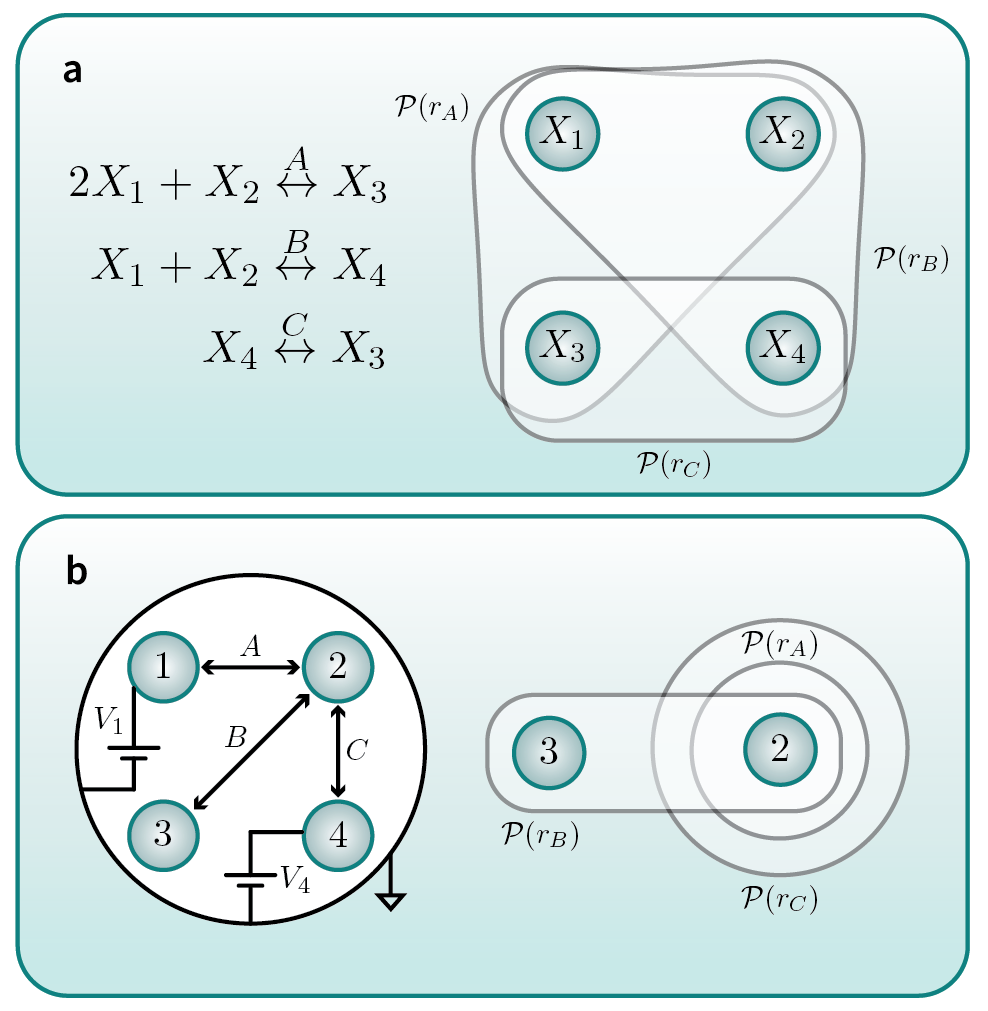
However, MPPs require that every mechanism (a generalized external system mediating the system’s state transitions, e.g., a thermal or chemical reservoir) coupled to the system interacts with only one subsystem. So, in an MPP, only one subsystem can change state at any given time. Unfortunately, at most spatio-temporal scales that we observe, multiple subsystems do change state at the same time. As a canonical example, in chemical reaction networks (Fig. 1(a)), multiple species counts must change state concurrently. As another example, the voltages on different conductors in a circuit (Fig. 1(b)) must change state at the same time.

There has been some preliminary work extending the stochastic thermodynamics of MPPs to address the broader scenario in which each mechanism couples to a set of multiple subsystems Wolpert 2020b. Systems with this nature are called composite systems, and their dynamics is called a composite process.

Here we extend this preliminary work and obtain new results in the stochastic thermodynamics of composite processes. We decompose key quantities (including probability flows, entropy production, and dynamical activity) into contributions from each mechanism. We also analyze the network specifying which (set of) subsystems can affect the dynamics of each subsystem. This network gives rise to units, which are subsets of subsystems whose joint dynamics does not depend on the state of the rest of the system. We then use the specification of units and the decomposition of key quantities to derive a wealth of thermodynamic uncertainty relations (TURs). Finally, we derive a strengthened thermodynamic speed limit theorem (SLT) for composite processes. This speed limit provides a tighter restriction on how much the probability distribution over system states can change during a fixed time interval, using the contributions from each mechanism to entropy production and dynamical activity. These results also apply to MPPs, since they are a special case of a composite process.

We begin by reviewing the preliminary work on composite processes, including the specification of units. We then present how key quantities decompose into contributions from each mechanism coupled to the system. We then present our results for TURs and strengthened SLTs. We conclude by discussing our results in the broader contexts of the thermodynamics of constraints and the thermodynamics of computation and by suggesting avenues of future work.

I Stochastic thermodynamics
of composite processes

I.1 Background on composite processes

A composite process is a generalization of MPPs, describing the co-evolution of a finite set of subsystems, $\mathcal{N}=\{1,2,\ldots,N\}$ . Each subsystem $i$ has a discrete state space $X_{i}$ . $x$ indicates a state vector in $X=\bigtimes_{\;i\in\mathcal{N}}X_{i}$ , the joint state space of the full system. $x_{A}$ indicates a state vector in $X=\bigtimes_{\;i\in A}X_{i}$ , the joint state space of the subset $A$ . The probability that the entire system is in a state $x$ at time $t$ evolves according to a master equation:

\displaystyle\frac{d}{dt}p_{x}(t)=K^{x^{\prime}}_{x}(t)p_{x^{\prime}}(t)

(1)

This stochastic dynamics arises due to couplings of the system with a set of mechanisms ${\mathcal{V}}=\{v_{1},v_{2},\ldots,v_{M}\}$ . In general, each such mechanism $v$ couples to only a subset of the subsystems. We refer to the set of subsystems to which a mechanism $v$ couples as its puppet set, and write it as ${\mathcal{P}}(v)\subseteq\mathcal{N}$ .

As an example, an MPP is a composite process where each mechanism couples to only one subsystem (although a single subsystem might be coupled to multiple mechanisms Horowitz 2015). So in an MPP, the cardinality of every puppet set is $1$ .

Refer to caption — Figure 1: Examples of systems whose dynamics can be modeled as composite processes. Each system consists of multiple subsystems (blue circles). Mechanisms are denoted as $r$ , and their puppet sets ${\mathcal{P}}(r)$ are indicated by translucent white bubbles. (a) An example stochastic chemical reaction network consists of four co-evolving species $\{X_{1},X_{2},X_{3},X_{4}\}$ that change state according to three chemical reactions $\{A,B,C\}$ . (b) An example toy circuit consists of four conductors $\{1,2,3,4\}$ that change state via interactions with three devices $\{A,B,C\}$ .

At any given time, a composite system changes state due to its interaction with at most one mechanism, just as with MPPs. Accordingly, the rate matrix of the overall system is a sum of mechanism-specific rate matrices:

	$\displaystyle K^{x^{\prime}}_{x}(t)$	$\displaystyle=\sumop\displaylimits_{v\in{\mathcal{V}}}\delta^{x^{\prime}_{\mathcal{N}\backslash{\mathcal{P}}(v)}}_{x_{\mathcal{N}\backslash{\mathcal{P}}(v)}}K^{x^{\prime}_{{\mathcal{P}}(v)},x^{\prime}_{\mathcal{N}\backslash{\mathcal{P}}(v)}}_{x_{{\mathcal{P}}(v)},x_{\mathcal{N}\backslash{\mathcal{P}}(v)}}(t)$		(2)
		$\displaystyle:=\sumop\displaylimits_{v\in{\mathcal{V}}}K^{x^{\prime}}_{x}(v;t)$		(3)

(Here and throughout, for any two variables, $z,z^{\prime}$ contained in the same space, $\delta^{z^{\prime}}_{z}$ is the Kronecker delta function that equals $1$ when $z^{\prime}=z$ , and equals $0$ otherwise).

We can illustrate composite processes using a toy stochastic chemical reaction network (Fig. 1a) Wachtel et al. 2018; Rao and Esposito 2016; Rao and Esposito 2018a. This network involves four co-evolving species $\{X_{1},X_{2},X_{3},X_{4}\}$ that change state according to three chemical reactions $\{A,B,C\}$ (left). The system state is a vector consisting of the number of molecules of each species in the system. Only one reaction can occur at a time, but when a reaction does occur, multiple subsystems all change their state. For example, in the forward reaction $A$ , species $X_{1}$ , $X_{2}$ , and $X_{3}$ must change state at the same time, by counts of $\{-2,-1,+1\}$ , respectively. Accordingly, this reaction network is not an MPP. However, it is a composite process.

We can illustrate this composite process in terms of the associated puppet sets (righthand side of figure). There are a total of three such puppet sets, one for each of the possible chemical reactions. These three puppet sets are indicated by translucent bubbles in the righthand part of the figure. The mechanisms of the three puppet sets are denoted as $r_{A}$ , $r_{B}$ , and $r_{C}$ , and the puppet set of mechanism $r$ is denoted as ${\mathcal{P}}(r)$ .

As another example, consider a toy electronic circuit (Fig. 1b) Freitas et al. 2020 consisting of four conductors (the four circles in the left-hand side of the figure) and three devices (the three bidirectional arrows). The state of the system is a vector consisting of the voltage on each conductor. Two of the conductors ( $1$ and $4$ ) are “regulated”, since they are tied directly to fixed voltage sources ( $V_{1}$ and $V_{4}$ ). The other two conductors ( $2$ and $3$ ) are “free” to stochastically change state via the effect of devices $A$ , $B$ , and $C$ .

The composite process capturing the dynamics of the state of this circuit is illustrated in the right-hand side of the figure. There are three puppet sets (each a translucent bubble), each corresponding to a mechanism associated with one of the devices in the system. The mechanisms are denoted as $r_{A}$ , $r_{B}$ , and $r_{C}$ , and the puppet set of mechanism $r$ is denoted as ${\mathcal{P}}(r)$ .

In an MPP, even though the mechanisms that affect the dynamics of any subsystem $i$ do not affect the dynamics of any other subsystem, in general the dynamics of $i$ will depend on the states of some set of other subsystems. For example, in a bipartite process Horowitz and Esposito 2014, both of the subsystems can be modeled as having their own set of mechanisms, but each subsystem’s dynamics is governed by the state of the other subsystem as well as its own state.

Similarly, in a composite process, the dynamics of each subsystem $i$ can depend on the state of other subsystems in addition to its own state. Each such dependency can be represented as an edge in a directed graph. In the resulting dependency network each edge $j\to i$ means that the state of subsystem $j$ affects the rate of state transitions in subsystem $i$ . We refer to the set of subsystems whose state affects the dynamics of $i$ as the leaders of $i$ . So $j\to i$ means that $j$ is a leader of $i$ . In any dependency network, the leaders of each subsystem $i$ are its parents, $\text{pa}(i)$ .

The leader set for a mechanism $v$ is defined to be the union of the leaders of each subsystem in the puppet set of $v$ : ${\mathcal{L}}(v)=\bigcupop\displaylimits_{i\in{\mathcal{P}}(v)}\text{pa}(i)$ . As an example, even though the puppet set of mechanism $v_{2}$ in Fig. 2 is $\{A,C,D\}$ , the leader set of $v_{2}$ is $\{A,B,C,D\}$ .

The leader set of any mechanism is a (perhaps proper) superset of its puppet set. Accordingly, we can write

\displaystyle K^{x^{\prime}}_{x}(v;t)=K^{x^{\prime}_{{\mathcal{L}}(v)},x^{\prime}_{\mathcal{N}\setminus{\mathcal{L}}(v)}}_{x^{\prime}_{{\mathcal{L}}(v)\backslash{\mathcal{P}}(v)},x_{{\mathcal{P}}(v)},x^{\prime}_{\mathcal{N}\setminus{\mathcal{L}}(v)}}(v;t)

(4)

With abuse of notation, we can rewrite this in a way that explicitly embodies the fact that the instantaneous dynamics of the puppet set ${\mathcal{P}}(v)$ depends at most on the state of the leader set ${\mathcal{L}}(v)$ , and not on the state of any of the subsystems in $\mathcal{N}\backslash{\mathcal{L}}(v)$ :

\displaystyle K^{x^{\prime}_{{\mathcal{L}}(v)}}_{x^{\prime}_{{\mathcal{L}}(v)\backslash{\mathcal{P}}(v)},x_{{\mathcal{P}}(v)}}(v;t):=K^{x^{\prime}}_{x}(v;t)

(5)

A unit $\omega\subseteq\mathcal{N}$ is a collection of subsystems such that as the full system’s state evolves via a master equation according to $K(t)$ , the marginal distribution over the states of the unit also evolves according to its own CTMC:

\displaystyle\frac{d}{dt}p_{x_{\omega}}(t)=K^{x^{\prime}_{\omega}}_{x_{\omega}}(\omega;t)p_{x^{\prime}_{\omega}}(t)

(6)

for some associated rate matrix $K(\omega;t)$ . Intuitively, a unit is any set of subsystems whose evolution is independent of the states of the subsystems outside the unit. Typically, a unit is a union of leader sets. In such cases no subsystem in the unit has parents outside of the unit. Importantly though, this doesn’t prevent there being a subsystem in the unit that is a leader for some subsystem outside of the unit. Informally speaking, the boundary of a unit in an dependency network can have outgoing edges, even though it cannot have any incoming edges.

Any union of units is a unit, and any non-empty intersection of units is a unit Wolpert 2020b. Note that the entire system $\mathcal{N}$ itself is a unit. We denote the set of all units as $\mathcal{N}^\dagger$ .

Since each separate unit evolves according to its own CTMC, all the usual theorems of stochastic thermodynamics apply to each unit separately. In particular, the Second Law Wolpert 2020b applies, as do the thermodynamic uncertainty relations Horowitz and Gingrich 2017; Dechant 2018; Hasegawa and Van Vu 2019, the speed limit theorems Shiraishi et al. 2018; Shiraishi and Saito 2021; Lee et al. 2022, the fluctuation theorems Rao and Esposito 2018b, first-passage time bounds and bounds on stopping times Gingrich and Horowitz 2017; Neri et al. 2017; Neri et al. 2019, etc.

We highlight that for any pair of nested units $\omega$ and $\alpha\subseteq\omega$ , it is true that Wolpert 2020b; Wolpert 2020a:

\displaystyle\dot{\sigma}^{\omega}(t)\geq\dot{\sigma}^{\alpha}(t)

(7)

A set of units $\mathcal{N}^*$ is called a unit structure if it obeys the following properties Wolpert 2020b:

•

The union of the units in the set equals $\mathcal{N}$ .

$\mathcal{N}^*=\{\omega_{1},\omega_{2},\ldots\}:\bigcupop\displaylimits_{\omega\in\mathcal{N}^\dagger}\omega=\mathcal{N}$
•

The set is closed under intersections of its units.

$\forall\,(\omega_{1},\omega_{2})\in\left(\mathcal{N}^*\right)^2=\omega_{1}\cap\omega_{2}\in\mathcal{N}^*$

We define an inclusion-exclusion sum of a function $f^\omega$ evaluated on every unit $\omega$ in a unit structure $\mathcal{N}^*$ as

\displaystyle\widehat{\sumop\displaylimits}_{\omega\in\mathcal{N}^*}f^\omega=\sumop\displaylimits_{\omega^{\prime}\in\mathcal{N}^*_{1}}f^{\omega^{\prime}}-\sumop\displaylimits_{\omega^{\prime\prime}\in\mathcal{N}^*_{2}}f^{\omega^{\prime\prime}}+\sumop\displaylimits_{\omega^{\prime\prime\prime}\in\mathcal{N}^*_{3}}f^{\omega^{\prime\prime\prime}}-\ldots

(8)

For example, the time- $t$ inclusion-exclusion (or “in-ex” for short) information reads

\displaystyle{\mathcal{I}}^{\mathcal{N}^*}(t):=\left(\widehat{\sumop\displaylimits}_{\omega\in{\mathcal{N}^*}}S^\omega(t)\right)-S^{\mathcal{N}^*}(t)

(9)

Using the fact that the heat flow into the unit structure also decomposes into an in-ex sum, we can decompose the global EP incurred during a time period $[0,\tau]$ according to

\displaystyle\sigma^\mathcal{N}=\widehat{\sumop\displaylimits}_{\omega\in{\mathcal{N}^*}}\sigma^{\omega}-\Delta{\mathcal{I}}^{{\mathcal{N}^*}}

(10)

where $\Delta{\mathcal{I}}^{{\mathcal{N}^*}}$ is the change in the in-ex information during the time period $[0,\tau]$ . For a detailed proof of the in-ex decomposition of the global EP, see Wolpert 2020a; Wolpert 2023.

One can use the in-ex sum decomposition of the EP in various ways depending on what degrees of freedom are accessible in the system of interest. For example, if one can calculate the mismatch cost Kolchinsky and Wolpert 2017; Kolchinsky and Wolpert 2021 $\lambda^\omega$ for each unit in the unit structure, then the in-ex sum can be rewritten:

\displaystyle\sigma^\mathcal{N}=\widehat{\sumop\displaylimits}_{\omega\in{\mathcal{N}^*}}\lambda^{\omega}+\widehat{\sumop\displaylimits}_{\omega\in{\mathcal{N}^*}}\xi^{\omega}-\Delta{\mathcal{I}}^{{\mathcal{N}^*}}

(11)

where $\xi^\omega=\sigma^\omega-\lambda^\omega$ is the “residual EP” due to everything aside from the mismatch cost.

Additionally, a very large number of lower bounds can be obtained on the global EP by replacing any positive $\sigma^\omega$ (or any such set of them) in the in-ex sum with any lower bound (e.g., TUR, SLT, etc.) on the value of that unit’s EP. (See Wolpert 2023 for examples in the special case of MPPs.)

I.2 Decomposition of thermodynamic and dynamical quantities in composite processes

Since the entire system $\mathcal{N}$ is itself a unit, we will write all our results in terms of units for the rest of the paper.

The rate matrix of each unit $\omega$ in a composite process decomposes into rate matrices from each mechanism whose leader set is a subset of $\omega$ :

	$\displaystyle K^{x^{\prime}_{\omega}}_{x_{\omega}}(\omega;t)$	$\displaystyle=\sumop\displaylimits_{v:{\mathcal{L}}(v)\subseteq\omega}\delta^{x^{\prime}_{\omega\backslash{\mathcal{L}}(v)}}_{x_{\omega\backslash{\mathcal{L}}(v)}}K^{x^{\prime}_{{\mathcal{L}}(v)},x^{\prime}_{\omega\backslash{\mathcal{L}}(v)}}_{x_{{\mathcal{L}}(v)},x_{\omega\backslash{\mathcal{L}}(v)}}(t)$		(12)
		$\displaystyle=\sumop\displaylimits_{v:{\mathcal{L}}(v)\subseteq\omega}K^{x^{\prime}_{\omega}}_{x_{\omega}}(v;t)$		(13)

Similarly, we can decompose the EP rate of any unit $\omega$ :

	$\displaystyle\dot{\sigma}^{\omega}(t)$	$\displaystyle=\sumop\displaylimits_{\begin{subarray}{c}v:{\mathcal{L}}(v)\subseteq\omega,\\ x^{\prime}_{\omega},x_{\omega}\neq x^{\prime}_{\omega}\end{subarray}}K^{x^{\prime}_{\omega}}_{x_{\omega}}(v;t)\,p_{x^{\prime}_{\omega}}(t)\ln\left[\frac{K^{x^{\prime}_{\omega}}_{x_{\omega}}(v;t)\,p_{x^{\prime}_{\omega}}(t)}{K^{x_{\omega}}_{x^{\prime}_{\omega}}(v;t)\,p_{x_{\omega}}(t)}\right]$		(14)
		$\displaystyle=\sumop\displaylimits_{v:{\mathcal{L}}(v)\subseteq\omega}\dot{\zeta}^{v}_{\omega}(t)$		(15)

into contributions $\dot{\zeta}^{v}_{\omega}(t)$ from each mechanism whose leader set is a subset of $\omega$ . In particular, since the entire system is a unit whose state transitions are mediated by every mechanism $v\in{\mathcal{V}}$ , the global EP rate decomposes as $\dot{\sigma}^{\mathcal{N}}(t)=\sumop\displaylimits_{v}\dot{\zeta}^{v}_{\mathcal{N}}(t)$ .

A unit’s dynamical activity also decomposes:

\displaystyle{\mathcal{A}}^\omega(t)=\sumop\displaylimits_{\begin{subarray}{c}v:{\mathcal{L}}(v)\subseteq\omega,\\ x^{\prime}_{\omega},x_{\omega}\neq x^{\prime}_{\omega}\end{subarray}}K^{x^{\prime}_{\omega}}_{x_{\omega}}(v;t)\,p_{x^{\prime}_{\omega}}(t)=\sumop\displaylimits_{v:{\mathcal{L}}(v)\subseteq\omega}{\mathcal{A}}(v;t)

(16)

Similarly, the entire system’s dynamical activity can be decomposed as ${\mathcal{A}}^\mathcal{N}(t)=\sumop\displaylimits_{v}{\mathcal{A}}(v;t)$ . Note that the dynamics of every pair of nested units $\omega,\alpha\subseteq\omega$ must be consistent with one another Wolpert 2020b, which means that ${\mathcal{A}}_{\alpha}(v;t)={\mathcal{A}}_{\omega}(v;t)={\mathcal{A}}(v;t)$ for all $\alpha$ and $\omega$ .

We denote the probability flow from $x^{\prime}_{\omega}\to x_{\omega}$ due to mechanism $v$ as ${\mathcal{A}}^{x^{\prime}_{\omega}}_{x_{\omega}}(v;t)=K^{x^{\prime}_{\omega}}_{x_{\omega}}(v;t)\,p_{x^{\prime}_{\omega}}(t)$ . We write the net probability current from $x^{\prime}_{\omega}\to x_{\omega}$ due to mechanism $v$ as $J^{x^{\prime}_{\omega}}_{x_{\omega}}(v;t)={\mathcal{A}}^{x^{\prime}_{\omega}}_{x_{\omega}}(v;t)-{\mathcal{A}}^{x_{\omega}}_{x^{\prime}_{\omega}}(v;t)$ . The total net probability current from $x^{\prime}_{\omega}\to x_{\omega}$ equals the sum of the probability currents due to each mechanism whose leader set is a subset of the unit $\omega$ :

\displaystyle J^{x^{\prime}_{\omega}}_{x_{\omega}}(t)=\sumop\displaylimits_{v:{\mathcal{L}}(v)\subseteq\omega}J^{x^{\prime}_{\omega}}_{x_{\omega}}(v;t)

(17)

Accordingly, we can decompose the master equation for the unit $\omega$ into probability currents induced by each mechanism:

\displaystyle\frac{d}{dt}p_{x_{\omega}}(t)=\sumop\displaylimits_{\begin{subarray}{c}v:{\mathcal{L}}(v)\subseteq\omega,\\ x^{\prime}_{\omega}\neq x_{\omega}\end{subarray}}K^{x^{\prime}_{\omega}}_{x_{\omega}}(v;t)p_{x^{\prime}_{\omega}}(t)=\sumop\displaylimits_{\begin{subarray}{c}v:{\mathcal{L}}(v)\subseteq\omega,\\ x^{\prime}_{\omega}\end{subarray}}J^{x^{\prime}_{\omega}}_{x_{\omega}}(v;t)

(18)

II Thermodynamic Uncertainty Relations for Composite Processes

For any unit $\omega$ that is in an NESS, any linear function of probability currents ${\mathcal{C}}_{\omega}$ is a current. It can be divided into contributions from each mechanism:

$\displaystyle\dot{{\mathcal{C}}}_{\omega}$	$\displaystyle=\sumop\displaylimits_{x^{\prime}_{\omega},x_{\omega}>x^{\prime}_{\omega}}J^{x^{\prime}_{\omega}}_{x_{\omega}}C^{x^{\prime}_{\omega}}_{x_{\omega}}$	(19)
	$\displaystyle=\sumop\displaylimits_{\begin{subarray}{c}v:{\mathcal{L}}(v)\subseteq\omega,\\ x^{\prime}_{\omega},x_{\omega}>x^{\prime}_{\omega}\end{subarray}}J^{x^{\prime}_{\omega}}_{x_{\omega}}(v)C^{x^{\prime}_{\omega}}_{x_{\omega}}$	(20)
	$\displaystyle=\sumop\displaylimits_{v:{\mathcal{L}}(v)\subseteq\omega}\dot{{\mathcal{C}}}_{\omega}(v)$	(21)

where $C^{x^{\prime}_{\omega}}_{x_{\omega}}=-C_{x^{\prime}_{\omega}}^{x_{\omega}}$ is some anti-symmetric function of state transitions, and we have dropped the time dependence in the steady state.

Importantly, the current contribution from each mechanism $\dot{{\mathcal{C}}}_{\omega}(v)$ is itself a current. So all of the thermodynamic uncertainty relations (TURs) hold for the time-integrated version of any such mechanism-specific current. In an NESS running for a time period of length $\tau$ , this mechanism-specific time-integrated current is ${\mathcal{C}}_{\omega}(v)=\tau\dot{{\mathcal{C}}}_{\omega}(v)$ . Additionally, since every unit evolves according to its own CTMC, the TURs hold for each unit.

For example, the finite-time TUR bounds the precision of any current in a CTMC with respect to its EP rate Horowitz and Gingrich 2017; Pietzonka et al. 2017. For a composite process, this holds for any unit and any arbitrary time-integrated current:

\displaystyle\sigma^\omega\geq\frac{2\langle{\mathcal{C}}_{\omega}\rangle^2}{\text{Var}({\mathcal{C}}_{\omega}}

(22)

Additionally, for any mechanism $v:{\mathcal{L}}(v)\subseteq\omega$ and any associated current ${\mathcal{C}}_{\omega}(v)$ ,

\displaystyle\sigma^\omega\geq\frac{2\langle{\mathcal{C}}_{\omega}(v)\rangle^2}{\text{Var}({\mathcal{C}}_{\omega}(v))}

(23)

The vector-valued TUR following Dechant 2018 holds for a vector $\bm{\dot{{\mathcal{C}}}}_{\omega}$ of any set of (potentially mechanism-specific) currents $\{\dot{{\mathcal{C}}}_{\omega}\}$ that are not linearly dependent:

\bm{\dot{{\mathcal{C}}}}_{\omega}^T\>\mathbf{\Xi}_{\omega}^{-1}\>\bm{\dot{{\mathcal{C}}}}_{\omega}\leq\frac{\dot{\sigma}^\omega}{2\tau}

(24)

where $\mathbf{\Xi}_{\omega}^{-1}$ is the inverse of the covariance matrix of the associated time-integrated currents $\{{\mathcal{C}}_{\omega}\}$ .

Any of these TURs can be useful to bound the entropy production when one has limited access to the system in the sense that one can measure state transitions i) due only to some subset of the mechanisms influencing the system or state transitions or ii) involving some subset of units in the system.

II.1 Information Flow TURs

One important quantity in an MPP is information flow Horowitz and Esposito 2014; Horowitz 2015; Hartich et al. 2016. Here, we extend the concept of information flow to composite processes. For any unit $\omega$ in an NESS, a set of subsystems $A\subset\omega$ , and a set of subsystems $B\subset\omega$ (for which $A\cap B=\varnothing$ ), the information flow is the rate of decrease in the conditional entropy of the state of $B$ given the state of $A$ , due to state transitions in $A$ :

\displaystyle\dot{I}^{A\to B}=\sumop\displaylimits_{x^{\prime}_{\omega},x_{\omega}>x^{\prime}_{\omega}}J^{x^{\prime}_{\omega}}_{x_{\omega}}\delta^{x^{\prime}_{\omega\backslash A}}_{x_{\omega\backslash A}}\ln\frac{p_{x_{B}|x_{A}}}{p_{x_{B}|x^{\prime}_{A}}}

(25)

So, when $\omega$ is in an NESS, the information flow is a current for which $C^{x^{\prime}_{\omega}}_{x_{\omega}}=C^{x^{\prime}_{\omega\backslash A},x^{\prime}_{A}}_{x_{\omega\backslash A},x_{A}}=\delta^{x^{\prime}_{\omega\backslash A}}_{x_{\omega\backslash A}}\ln\frac{p_{x_{B}|x_{A}}}{p_{x_{B}|x^{\prime}_{A}}}$ . The contribution to that information flow that is due to interactions of the unit with reservoir $v:{\mathcal{L}}(v)\subseteq\omega$ is itself an information flow

\displaystyle\dot{I}^{A\to B}(v)=\sumop\displaylimits_{x^{\prime}_{\omega},x_{\omega}>x^{\prime}_{\omega}}J^{x^{\prime}_{\omega}}_{x_{\omega}}(v)\delta^{x^{\prime}_{\omega\backslash A}}_{x_{\omega\backslash A}}\ln\frac{p_{x_{B}|x_{A}}}{p_{x_{B}|x^{\prime}_{A}}}

(26)

Since these information flows are currents, the TURs will apply to them. This observation in combination with Eq. 7 suggests that the precision of an information flow is (best) bounded by the reciprocal of the entropy production of the smallest unit which contains $A\cup B$ .

III Strengthened Thermodynamic Speed Limits for Composite Processes

Here we derive a speed limit similar to the one in Lee et al. 2022, but for composite processes. This speed limit is tighter than the one presented in that paper. Our analysis will hold for an arbitrary unit $\omega$ (which could be the entire system $\mathcal{N}$ itself):

\displaystyle l_{\omega}\leq\sumop\displaylimits_{v:{\mathcal{L}}(v)\subseteq\omega}{\mathcal{A}}_{\omega}^{\text{tot}}(v;\tau)\,f\left(\frac{\zeta^v_{\omega}(\tau)}{{\mathcal{A}}_{\omega}^{\text{tot}}(v;\tau)}\right)

(27)

where the dynamics occurs during the time period $[0,\tau]$ . Additionally, $l_{\omega}$ is the total variation distance between the initial (time- $0$ ) and final (time- $\tau$ ) probability distributions over states of the unit $\omega$ . ${\mathcal{A}}_{\omega}^{\text{tot}}(v;\tau)$ is the total time-integrated dynamical activity due to mechanism $v$ . $\zeta^v_{\omega}(\tau)$ is the total contribution to the entropy production of unit $\omega$ due to interactions of $\omega$ with mechanism $v$ .

We start by bounding the total variation distance between the initial and final (time- $\tau$ ) probability distributions over states of the unit $\omega$ :

$\displaystyle l_{\omega}$	$\displaystyle:={\mathbb{L}}(p_{x_{\omega}}(0),p_{x_{\omega}}(\tau))=\frac{1}{2}\sumop\displaylimits_{x_{\omega}}\left\lvert p_{x_{\omega}}(\tau)-p_{x_{\omega}}(0)\right\rvert$	(28)
	$\displaystyle=\frac{1}{2}\sumop\displaylimits_{x_{\omega}}\left\|\intop\nolimits_{0}^\tau dt\frac{d}{dt}p_{x_{\omega}}(t)\right\|$	(29)
	$\displaystyle\leq\frac{1}{2}\intop\nolimits_{0}^\tau dt\sumop\displaylimits_{x_{\omega}}\left\lvert\frac{d}{dt}p_{x_{\omega}}(t)\right\rvert$	(30)

In a composite process, we can further bound the integrand:

	$\displaystyle\sumop\displaylimits_{x_{\omega}}\left\lvert\frac{d}{dt}p_{x_{\omega}}(t)\right\rvert$	$\displaystyle=\sumop\displaylimits_{x_{\omega}}\left\lvert\sumop\displaylimits_{v:{\mathcal{L}}(v)\subseteq\omega}\sumop\displaylimits_{x^{\prime}_{\omega}\neq x_{\omega}}J^{x^{\prime}_{\omega}}_{x_{\omega}}(v;t)\right\rvert$		(31)
		$\displaystyle\leq\sumop\displaylimits_{v:{\mathcal{L}}(v)\subseteq\omega}\sumop\displaylimits_{x_{\omega},x^{\prime}_{\omega}\neq x_{\omega}}\left\lvert J^{x^{\prime}_{\omega}}_{x_{\omega}}(v;t)\right\rvert$		(32)

We write the time- $t$ “conditional probability distribution” of the forward process, under the counterfactual scenario that the process evolves with coupling only to mechanism $v:{\mathcal{L}}(v)\subseteq\omega$ as

\displaystyle W^{x^{\prime}_{\omega}}_{x_{\omega}}(v;t)=\frac{(1-\delta^{x^{\prime}_{\omega}}_{x_{\omega}})\,K^{x^{\prime}_{\omega}}_{x_{\omega}}(v;t)\,p_{x^{\prime}_{\omega}}(t)}{{\mathcal{A}}_{\omega}(v;t)}

(33)

Intuitively, this can be interpreted as a conditional probability that if a jump occurs at $t$ due reservoir $v:{\mathcal{L}}(v)\subseteq\omega$ , that the state before the jump was $x^{\prime}_{\omega}$ and the state afterwards was $x_{\omega}$ We write the same quantity for the reverse process as

\displaystyle\widetilde{W}^{x_{\omega}^{\prime}}_{x_{\omega}}(t)=\frac{(1-\delta^{x_{\omega}}_{x^{\prime}_{\omega}})\,K^{x_{\omega}}_{x^{\prime}_{\omega}}(v;t)\,p_{x_{\omega}}(t)}{{\mathcal{A}}_{\omega}(v;t)}

(34)

The total variation distance between these matrices $d_{\text{TV}}(\mathbf{W}_{\omega}(v;t),\mathbf{\widetilde{W}}_{\omega}(v;t))$ represents how irreversible this counterfactual process (the one driven only by mechanism $v$ ) is at time $t$ . Using these definitions, we can rewrite Eq. 32 as

\displaystyle\sumop\displaylimits_{x_{\omega}}

\displaystyle\left\lvert\frac{d}{dt}p_{x_{\omega}}(t)\right\rvert

\displaystyle\leq 2\sumop\displaylimits_{v:{\mathcal{L}}(v)\subseteq\omega}{\mathcal{A}}_{\omega}(v;t)\,d_{\text{TV}}(\mathbf{W}_{\omega}(v;t),\mathbf{\widetilde{W}}_{\omega}(v;t))

(35)

Plugging into Eq. 30, we obtain

\displaystyle l_{\omega}\leq\intop\nolimits_{0}^\tau dt\sumop\displaylimits_{v:{\mathcal{L}}(v)\subseteq\omega}{\mathcal{A}}_{\omega}(v;t)\,d_{\text{TV}}(\mathbf{W}_{\omega}(v;t),\mathbf{\widetilde{W}}_{\omega}(v;t))

(36)

We next make use of the fact that mechanism $v$ ’s contribution to the EP rate of unit $\omega$ (Eq. 15) can be written in terms of the Kullback-Leibler (KL) divergence between the conditional distributions of the forward and backward processes as

\displaystyle\dot{\zeta}^{v}_{\omega}(t)={\mathcal{A}}_{\omega}(v;t)\,D_{\text{KL}}(\mathbf{W}_{\omega}(v;t),\mathbf{\widetilde{W}}_{\omega}(v;t))

(37)

Any positive monotonic concave function $f$ relates the total variation distance to the KL divergence Lee et al. 2022 according to:

\displaystyle d_{\text{TV}}(\bm{p};\bm{q})\leq f(D_{\text{KL}}(\bm{p};\bm{q}))

(38)

We can use this relationship to relate Eq. 37 to $l_{\omega}$ . Combining Eqs. 36, 37 and 38,

\displaystyle l_{\omega}

\displaystyle\leq\intop\nolimits_{0}^\tau dt\sumop\displaylimits_{v:{\mathcal{L}}(v)\subseteq\omega}{\mathcal{A}}_{\omega}(v;t)\,f\left(\frac{\dot{\zeta}^{v}_{\omega}(t)}{{\mathcal{A}}_{\omega}(v;t)}\right)

(39)

Next define $\zeta^v_{\omega}=\intop\nolimits_{0}^\tau dt\dot{\zeta}^{v}_{\omega}(t)$ as the total (ensemble-average) contribution to the EP of unit $\omega$ caused by an interaction of the system with mechanism $v$ during the time period $[0,\tau]$ . Also define ${\mathcal{A}}_{\omega}^{\text{tot}}(v;\tau)=\intop\nolimits_{0}^\tau dt{\mathcal{A}}_{\omega}(v;t)$ as the total (ensemble-average) number of state transitions in the unit $\omega$ that are caused by an interaction of the system with mechanism $v$ . Then using the positivity of the dynamical activity and of the EP, together with the concavity of $f$ , we can further bound the right hand side to obtain a general limit for composite processes:

\displaystyle l_{\omega}\leq\sumop\displaylimits_{v:{\mathcal{L}}(v)\subseteq\omega}{\mathcal{A}}_{\omega}^{\text{tot}}(v;\tau)\,f\left(\frac{\zeta^v_{\omega}(\tau)}{{\mathcal{A}}_{\omega}^{\text{tot}}(v;\tau)}\right)

(40)

This result provides an upper bound on how much $l_{\omega}$ can change during the time interval $[0,\tau]$ , in terms of the associated activity of $\omega$ and the contribution of $\omega$ to EP. So Eq. 40 is a thermodynamic speed limit theorem, involving

By comparison, the speed limit in Lee et al. 2022 applied to a unit $\omega$ reads

\displaystyle l_{\omega}\leq{\mathcal{A}}_{\omega}^{\text{tot}}(\tau)\,f\left(\frac{\sigma_{\omega}(\tau)}{{\mathcal{A}}_{\omega}^{\text{tot}}(\tau)}\right)

(41)

For a composite process, the right hand side of this “global” bound expands to

\displaystyle l_{\omega}\leq\left(\sumop\displaylimits_{v:{\mathcal{L}}(v)\subseteq\omega}{\mathcal{A}}_{\omega}^{\text{tot}}(v;\tau)\right)\,\,f\left(\frac{\sumop\displaylimits_{v:{\mathcal{L}}(v)\subseteq\omega}\zeta^v_{\omega}(\tau)}{\sumop\displaylimits_{v:{\mathcal{L}}(v)\subseteq\omega}{\mathcal{A}}_{\omega}^{\text{tot}}(v;\tau)}\right)

(42)

By Jensen’s inequality, the speed limit for composite processes (Eq. 40) is always tighter than the speed limit provided by Lee et al. 2022 (Eq. 41). For a concave function $f$ , a set of numbers a $x_{v}$ in its domain, and positive weights $a_{v}$ , Jensen’s inequality states that

\displaystyle\left(\sumop\displaylimits_{v}a_{v}\right)f\left(\frac{\sumop\displaylimits_{v}a_{v}x_{v}}{\sumop\displaylimits_{v}a_{v}}\right)\geq\sumop\displaylimits_{v}a_{v}f(x_{v})

(43)

Setting $a_{v}={\mathcal{A}}_{\omega}^{\text{tot}}(v;\tau)$ and $x_{v}=\frac{\zeta^v_{\omega}(\tau)}{{\mathcal{A}}_{\omega}^{\text{tot}}(v;\tau)}$ proves that Eq. 40) is always tighter than Eq. 41. Intuitively, this occurs because we’re able to define the mechanism-specific contributions to the EP and activity in a composite process.

Lee et al. 2022 provides some examples of acceptable functions $f$ . For example, if we follow Pinsker’s inequality and choose $f=\sqrt{\frac{x}{2}}$ , then the speed limit provided by Lee et al. 2022 collapses to the speed limit derived in Shiraishi et al. 2018. If we plug in this choice of $f$ to Eq. 40, extract the parameter $\tau$ by using the average frequency of state transitions $\langle{\mathcal{A}}_{\omega}(v)\rangle_{\tau}=\frac{{\mathcal{A}}_{\omega}^{\text{tot}}(v;\tau)}{\tau}$ , and rearrange terms, we obtain

\displaystyle\forall\omega\in\mathcal{N}^\dagger:\;\tau\geq\frac{({\mathbb{L}}(p_{x_{\omega}}(0),p_{x_{\omega}}(\tau)))^2}{2\left(\sumop\displaylimits_{v:{\mathcal{L}}(v)\subseteq\omega}\sqrt{\zeta^{v}_{\omega}(\tau)\langle{\mathcal{A}}^{v}_{\omega}\rangle_{\tau}}\right)^2}

(44)

the tightest of which is given by:

\displaystyle\tau\geq\max_{\omega\in\mathcal{N}^\dagger}\frac{({\mathbb{L}}(p_{x_{\omega}}(0),p_{x_{\omega}}(\tau)))^2}{2\left(\sumop\displaylimits_{v:{\mathcal{L}}(v)\subseteq\omega}\sqrt{\zeta^{v}_{\omega}(\tau)\langle{\mathcal{A}}^{v}\rangle_{\tau}}\right)^2}

(45)

This particular speed limit tells us that speed of the evolution of the system’s probability distribution cannot be greater than the speed of evolution of the distribution over the coordinates of the “slowest-evolving” unit.

IV Discussion

Here we have introduced the stochastic thermodynamics of composite processes. This work presents a preliminary analysis of how information flows in a composite process are constrained by the entropy productions of units. It also demonstrates that bounds on the speed of transforming a system’s probability distribution over states can be tightened with knowledge of the contributions to the entropy production and dynamical activity from each mechanism with which the system interacts.

This work fits into a growing branch of research on the stochastic thermodynamics of constraints. One example of research in this area investigates the effect of constraints on the control protocol (time sequence of rate matrices evolving the probability distribution) Kolchinsky and Wolpert 2020 There has also been some important work where the “constraint” on such a many-degree-of-freedom classical system is simply that it be some very narrowly defined type of system, whose dynamics is specified by many different kinds of parameters. For example, there has been analysis of the stochastic thermodynamics of chemical reaction networks Rao and Esposito 2016; Rao and Esposito 2018a, of electronic circuits Freitas et al. 2020; Gao and Limmer 2021; Wolpert and Kolchinsky 2020, and of biological copying mechanisms Poulton et al. 2019. This work analyzes the consequences of a major class of dynamical constraints that arises because many of these systems are most naturally modelled as a set of multiple co-evolving subsystems D’Souza 2009; Horowitz and Esposito 2014; Horowitz 2015; Ito and Sagawa 2013; Wolpert 2020c; Wolpert 2020b; Wolpert 2023; Wolpert 2020a. In particular, the main constraints on such systems are that only certain subsets of subsystems can simultaneously change state a given time, and the dependencies between subsystems impose restrictions on their joint dynamics.

There remain many avenues of potential future work, especially in the thermodynamics of computation. Many computational processes consist of multiple, co-evolving systems with the broad set of constraints that allow them to be easily modeled as a composite process. Research in this direction would first require formalizing the notion of computation in a composite process. One such computation, which equates to the identity map, is simply communication (information transmission). One could extend the recent study on the fundamental thermodynamic costs of communication Tasnim et al. 2023 to tie Shannon information theory to the stochastic thermodynamics of composite processes. More generally, for any given computation, one could analyze the trade-offs between the energy cost required to implement that computation and the performance (accuracy, time, etc.) of a composite process. In particular, there could be rich structure in how the properties of the dependency network in a composite process affects these trade-offs.

V Acknowledgements

This work was supported by the MIT Media Lab Consortium, Santa Fe Institute, US NSF EAGER Grant CCF-2221345. F.T. and D.H.W. thank Tarek Tohme for initial discussions regarding TURs for information flows in multipartite processes. F.T. thanks Nahuel Freitas for discussions regarding how circuits can be modeled as composite processes.

References

Horowitz (2015) J. M. Horowitz, Multipartite information flow for multiple maxwell demons, Journal of Statistical Mechanics: Theory and Experiment 2015, P03006 (2015).
Wolpert (2023) D. H. Wolpert, Combining lower bounds on entropy production in complex systems with multiple interacting components, in Frontiers in Entropy Across the Disciplines: Panorama of Entropy: Theory, Computation, and Applications (World Scientific, 2023) pp. 405–453.
Wolpert (2020a) D. H. Wolpert, Minimal entropy production rate of interacting systems, New Journal of Physics 22, 113013 (2020a).
Wolpert (2020b) D. H. Wolpert, Strengthened landauer bound for composite systems, arXiV (2020b).
Wachtel et al. (2018) A. Wachtel, R. Rao, and M. Esposito, Thermodynamically consistent coarse graining of biocatalysts beyond michaelis–menten, New Journal of Physics 20, 042002 (2018).
Rao and Esposito (2016) R. Rao and M. Esposito, Nonequilibrium thermodynamics of chemical reaction networks: wisdom from stochastic thermodynamics, Physical Review X 6, 041064 (2016).
Rao and Esposito (2018a) R. Rao and M. Esposito, Conservation laws and work fluctuation relations in chemical reaction networks, The Journal of chemical physics 149, 245101 (2018a).
Freitas et al. (2020) N. Freitas, J.-C. Delvenne, and M. Esposito, Stochastic thermodynamics of non-linear electronic circuits: A realistic framework for thermodynamics of computation, arXiv preprint arXiv:2008.10578 (2020).
Horowitz and Esposito (2014) J. M. Horowitz and M. Esposito, Thermodynamics with continuous information flow, Physical Review X 4, 031015 (2014).
Horowitz and Gingrich (2017) J. M. Horowitz and T. R. Gingrich, Proof of the finite-time thermodynamic uncertainty relation for steady-state currents, Physical Review E 96, 020103 (2017).
Dechant (2018) A. Dechant, Multidimensional thermodynamic uncertainty relations, Journal of Physics A: Mathematical and Theoretical 52, 035001 (2018).
Hasegawa and Van Vu (2019) Y. Hasegawa and T. Van Vu, Fluctuation theorem uncertainty relation, Physical review letters 123, 110602 (2019).
Shiraishi et al. (2018) N. Shiraishi, K. Funo, and K. Saito, Speed limit for classical stochastic processes, Physical Review Letters 121, 10.1103/physrevlett.121.070601 (2018).
Shiraishi and Saito (2021) N. Shiraishi and K. Saito, Speed limit for open systems coupled to general environments, Physical Review Research 3, 023074 (2021).
Lee et al. (2022) J. S. Lee, S. Lee, H. Kwon, and H. Park, Speed limit for a highly irreversible process and tight finite-time landauer’s bound, Physical review letters 129, 120603 (2022).
Rao and Esposito (2018b) R. Rao and M. Esposito, Detailed fluctuation theorems: A unifying perspective, Entropy 20, 635 (2018b).
Gingrich and Horowitz (2017) T. R. Gingrich and J. M. Horowitz, Fundamental bounds on first passage time fluctuations for currents, Physical review letters 119, 170601 (2017).
Neri et al. (2017) I. Neri, É. Roldán, and F. Jülicher, Statistics of infima and stopping times of entropy production and applications to active molecular processes, Physical Review X 7, 011019 (2017).
Neri et al. (2019) I. Neri, É. Roldán, S. Pigolotti, and F. Jülicher, Integral fluctuation relations for entropy production at stopping times, Journal of Statistical Mechanics: Theory and Experiment 2019, 104006 (2019).
Kolchinsky and Wolpert (2017) A. Kolchinsky and D. H. Wolpert, Dependence of dissipation on the initial distribution over states, Journal of Statistical Mechanics: Theory and Experiment 2017, 083202 (2017).
Kolchinsky and Wolpert (2021) A. Kolchinsky and D. H. Wolpert, Dependence of integrated, instantaneous, and fluctuating entropy production on the initial state in quantum and classical processes, Physical Review E 104, 054107 (2021).
Pietzonka et al. (2017) P. Pietzonka, F. Ritort, and U. Seifert, Finite-time generalization of the thermodynamic uncertainty relation, Physical Review E 96, 012101 (2017).
Hartich et al. (2016) D. Hartich, A. C. Barato, and U. Seifert, Sensory capacity: An information theoretical measure of the performance of a sensor, Physical Review E 93, 10.1103/physreve.93.022116 (2016).
Kolchinsky and Wolpert (2020) A. Kolchinsky and D. H. Wolpert, Entropy production and thermodynamics of information under protocol constraints, arXiv preprint arXiv:2008.10764 (2020).
Gao and Limmer (2021) C. Y. Gao and D. T. Limmer, Principles of low dissipation computing from a stochastic circuit model, arXiv preprint arXiv:2102.13067 (2021).
Wolpert and Kolchinsky (2020) D. H. Wolpert and A. Kolchinsky, Thermodynamics of computing with circuits, New Journal of Physics 22, 063047 (2020).
Poulton et al. (2019) J. M. Poulton, P. R. Ten Wolde, and T. E. Ouldridge, Nonequilibrium correlations in minimal dynamical models of polymer copying, Proceedings of the National Academy of Sciences 116, 1946 (2019).
D’Souza (2009) R. M. D’Souza, Structure comes to random graphs, Nature Physics 5, 627 (2009).
Ito and Sagawa (2013) S. Ito and T. Sagawa, Information thermodynamics on causal networks, Physical Review Letters 111, 180603 (2013).
Wolpert (2020c) D. H. Wolpert, Uncertainty relations and fluctuation theorems for bayes nets, Physical Review Letters 125, 10.1103/physrevlett.125.200602 (2020c).
Tasnim et al. (2023) F. Tasnim, N. Freitas, and D. H. Wolpert, The fundamental thermodynamic costs of communication, arXiv preprint arXiv:2302.04320 (2023).