Learning from Aggregated Data:
Curated Bags versus Random Bags

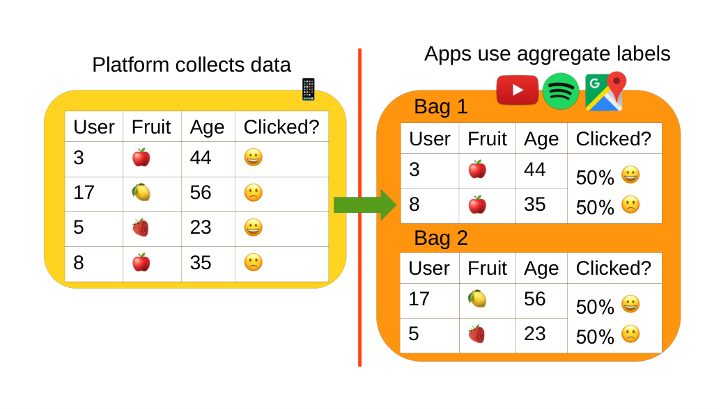
The use of machine learning methods to personalize online services has brought clear benefits for both users and providers, but has also raised concerns about privacy [18, 4, 11]. A recent proposal to address such privacy concerns is to use aggregated data, rather than individual data, to train models [3]. For example, the StoreKit Ad Network (SKAdNetwork) API from Apple aims to measure ad performance metrics such as impressions, clicks, and app installations at an aggregated level, allowing ad networks and advertisers to prioritize privacy concerns [1]. The Private Aggregation API of Chrome Privacy Sandbox may also collect user-generated data consisting of instance-label pairs and then enhances anonymity by providing apps and services with bags of instances that are labeled in an aggregated manner [2]. In the context of classification, for example, the proportion of each class among the instances in a bag can serve as an aggregate label, which can be then perturbed appropriately to ensure differential privacy. This is illustrated in Fig. 1.

In this paper, we explore two recently proposed methods for generating aggregated data labels: curated bags and random bags. The first method, curated bags, was considered in the Criteo Privacy Preserving ML Competition of AdKDD 2021 [12] and is also implemented in the Chrome Privacy Sandbox. It is primarily designed for datasets with categorical features¹¹ 1 We should highlight that it is not necessary for all feature columns to be categorical., but can also be applied to datasets with numerical features by bucketizing them. The process involves selecting a subset of categorical feature columns, aggregating examples that have the same combination of values for those columns into a bag, and labeling each bag with an aggregate label. However, in practice, some bags may be small and could pose a threat to privacy. To address this issue, the small bags can either be filtered out or an appropriate amount of noise can be added to ensure privacy. The second method, random bags, involves subsampling a predefined number of data points from the training dataset, aggregating the sampled examples into a bag, and labeling the bag with an aggregate label, which is a summary of the individual labels. This makes the individual labels invisible to the apps or services that are using the data. In this paper, we investigate the possibility of learning from aggregated data. Our contributions can be summarized as follows.

• •

  For a broad class of loss functions, so called semilinear loss (e.g., mean squared error, log loss, and Poisson loss), we demonstrate that if we use curated bags and if the model is a generalized additive model (whose sub-models are even allowed to share parameters), then we can perform gradient descent-based learning from aggregate labels without any performance loss.

• •

  We inverstigate the PAC learnability of random bags by using the Rademacher complexity and propose an estimator that minimizes an empirical bag-level risk. Our generalization bound shows the trade-off between the sample complexity and the size of the bag.

• •

  We conduct an empirical study of our lossless aggregate learning method, which utilizes the curated bags procedure. We train models on both individual and aggregate labels, and find that the curated bags approach is able to effectively learn from aggregate labels without any loss of performance. We also find that the generalized additive model with neural nets as sub-models outperforms the model with linear feature crosses, and that the curated bags approach outperforms the random bags approach. These results suggest that curated bags are more effective at preserving information during aggregation.

We discuss the societal impact of this work in Appendix A. All proofs are relegated to the appendix.

Aggregate labels are commonly used in group testing methods, such as screening for HIV in donated blood products [28] and identifying viral epidemics such as COVID-19 [26]. There are several prior work on learning with label proportions [24, 25, 10, 29, 14, 22, 19, 17]. While Yu et al. 2014 studied learning with random bags, they presented a distribution-independent VC dimension bound instead of a distribution-dependent Rademacher complexity bound, which is not only tighter but can also be applied to both classification and regression problems. In addition, our work applies a different random sampling procedure, and it also includes the rigorous study of curated bags. Quadrianto et al. 2008 examined how to estimate labels from label proportions using a specific generative model. Similarly, Zhang et al. 2020 applied the maximum likelihood method and developed theoretical guarantees by introducing the concept of consistency up to an equivalence relation. Musicant et al. 2007 presented a framework for learning from aggregate outputs and demonstrated adaptations of several classical machine learning algorithms. Other related work includes the proportion-SVM ($\propto$SVM) method [30], a boosting method for learning with label proportions [21], and extensions of nonparallel SVM that can learn with label proportions [20, 8]. Recently, Saket et al. 2022 studied the problem of combining bag distributions to better learn from label proportions. Another related area of research is label differential privacy [7, 6, 27, 13]. In this setting, the labels of individual instances are considered sensitive and require protection, while their features are considered non-sensitive. Learning from aggregate labels can be seen as an approach to achieving label privacy.

We use the shorthand notation $n$ to denote the set $\{1,2,\dots,n\}$. We denote the data domain by $\mathcal{X}$, and the label domain by $\mathcal{Y}$. We begin with the aggregating strategy called curated bags, a way of grouping examples in a dataset by their feature value combination. This aggregation method creates a partition of the entire dataset, where all examples in the same bag share the same feature value combination on the selected feature columns, while examples in different bags differ on those. In what follows, we show that the curated bags aggregation can achieve the same performance as learning from individual labels in the classical machine learning setting. To do so, we need to introduce two key components:

• •

  A semilinear loss function $\ell(y,\hat{y})$ is a loss function that is composed of a linear and a nonlinear function of the model prediction $\hat{y}$. Some widely used loss functions, such as the mean squared error, log loss, and Poisson loss, are all special cases of semilinear loss functions.

• •

  A generalized additive model (GAM) is a statsitical learning model that can be decomposed into a sum of several sub-models, allowing for different model capacity and expressivity of each sub-model. Each sub-model can be a neural network, decision tree, etc. The sub-models are allowed to share parameters, meaning that their parameter sets do not have to be non-overlapping. This allows GAMs to be more flexible than traditional regression models, which can only model a single relationship between a response variable and a set of predictors.

This section investigates a multilabel multiclass classification problem of learning from aggregate data. In this problem, the learner is given data bags that are formed by resampling examples from the training dataset without replacement. We emphasize that data examples are sampled without replacement within each bag. We follow the same procedure across bags, i.e., replacing all examples and sampling without replacement. This means that same examples may appear in multiple bags.

We assume that the data $(x,y)$ is drawn from an unknown distribution $\mathbb{P}$ over $\mathcal{X}\times\mathcal{Y}$, where $x$ is the example and $y$ is the label. We choose $\mathcal{Y}=\{0,1\}^{K}$, which generalizes $K$-class classification as a special case. In our general multilabel multiclass classification setting, the label $y$ can have multiple non-zero entries. We define $h(x)[k]$ and $y[k]$ to be the $k$-th entry of $h(x)$ and $y$, respectively. We evaluate the performance of a model $h:\mathcal{X}\to\mathcal{Y}$ by the expected Hamming distance

which is the expected number of entries in which $h(x)$ and $y$ disagree.

We denote the marginal distribution of $x$ (and $y$, respectively) under $\mathbb{P}$ by $\mathbb{P}\mid_{x}$ (and $\mathbb{P}\mid_{y}$, respectively). Let $\mathcal{H}\subseteq\left\{f:\mathcal{X}\to\mathcal{Y}\right\}$ be a hypothesis set. Let $\hat{\mathbb{P}}_{N}=\frac{1}{N}\sum_{i\in[N]}\delta_{\left(x^{(i)},y^{(i)}\right)}$ be an empirical measure of $\mathbb{P}$, where $\delta_{\left(x^{(i)},y^{(i)}\right)}$ is the Dirac measure at $\left(x^{(i)},y^{(i)}\right)\stackrel{{\scriptstyle\textnormal{i.i.d.}}}{{\sim}}\mathbb{P}$. The empirical measure $\hat{\mathbb{P}}_{N}$ models the uniform distribution on the training dataset $S_{\textnormal{train}}\triangleq\left\{\left(x^{(i)},y^{(i)}\right)\mid i\in[N]\right\}$.

Crucially, and in contrast to the classic learning setting, the raw training data is invisible to the learning algorithm. Instead, the learning algorithm has access to $n$ i.i.d. samples $(X_{i},\bar{y}_{i})$ that are obtained from the following process (denote the distribution of $(X_{i},\bar{y}_{i})$ by $\operatorname{Agg}(\hat{\mathbb{P}}_{N})$):

• •

  For each $i\in[n]$, we resample $m$ example-label pairs $S_{i}\triangleq\left\{\left(x_{i,j},y_{i,j}\right)\mid j\in[m]\right\}$ from the training dataset $S_{\textnormal{train}}$ uniformly at random without replacement;

• •

  We set $X_{i}=\left\{x_{i,j}\mid j\in[m]\right\}$ and $\bar{y}_{i}\mid y_{i,1},y_{i,2},\dots,y_{i,m}\sim\operatorname{Ber}\left(\frac{1}{m}\sum_{j\in[m]}y_{i,j}\right)$.

We study the problem of learning a hypothesis $f\in\mathcal{H}$ from the samples $\{(X_{i},\bar{y}_{i})\}_{i\in[n]}$. Since we consider an agnostic probably approximately correct (PAC) learning setup [16, Chapter 2], we are interested in upper-bounding the excess risk: $R(\hat{h})-\inf_{h\in\mathcal{H}}R(h)$ which is the gap between the risk of the hypothesis that our algorithm selects $R(\hat{h})$ and that of the optimal one in the hypothesis class $\inf_{h\in\mathcal{H}}R(h)$. We will bound the excess risk by the Rademacher complexity, defined as follows.

For multilabel classification, a hypothesis outputs a $K$-dimensional vector. We introduce the flattened Rademacher complexity to measure the correlation between Rademacher random variables and all entries of the hypothesis’s output.

In 2, we propose a new estimator $\hat{h}$ and upper-bound its excess risk $R(\hat{h})-\inf_{h\in\mathcal{H}}R(h)$ by a combination of the usual and flattened Rademacher complexities of the hypothesis class.

First, we would like to remark that if every bag only contains a single example (in this case $m=1$ and it reduces to the usual classification with individual labels), the correction term $-\frac{\left(m-1\right)N}{m\left(N-1\right)}\left\|\frac{1}{n}\sum_{i\in[n]}\left(\frac{1}{m}\sum_{x\in X_{i}}h(x)-\bar{y}_{i}\right)\right\|_{2}^{2}$ becomes zero. Second, there are three terms in Eq. 6. The first term has a factor of $\frac{2\left(m-1\right)N}{N-m}$ and the third term has a factor of $\frac{2m\left(N-1\right)}{N-m}$. If the bag size approaches the size of the entire training dataset ($m\to N$), both factors go to infinity and thereby drive the first and third terms to infinity, which also agrees with our intuition.

We assess the effectiveness of our proposed algorithm on the Criteo Ads dataset [9]. The dataset contains 41 million records with 13 integer and 26 categorical features. We convert the integer features into categorical features, resulting in a total of 39 categorical features. The data from the first 6 days is used for training, and the data from the 7th day is divided randomly into validation and test sets of equal size. We select a specific number of feature column pairs and use curated bags to form bags for the dataset. We introduce noise to ensure that the aggregate label is $\epsilon$-differentially private at various privacy budgets $\epsilon$. For each chosen pair of feature columns, a single aggregate label will be generated. Each training sample will have the same number of aggregate labels. A generalized additive model with multiple sub-models is constructed. Each sub-model is a multi-layer neural network that outputs a logit. The overall logit of the model is calculated by summing the logits of all the sub-models. The training loss is the sum of the losses for each aggregate label. The gradients of each sub-model’s training loss can only be applied to its own parameters. We evaluate the effectiveness of generalized additive models by using neural nets as sub-models and compare the results to those obtained by using linear feature crosses as sub-models. We refer to the generalized additive model that utilizes neural nets as sub-models as DNN and the one that uses linear feature crosses as sub-models as linear feature crosses.

We first show that our proposed curated bags method can learn effectively from aggregate labels without any loss in performance. In Fig. 3(a), we compare the proposed generalized additive models with DNN sub-models using individual labels and aggregate labels. We also compare them with the same model structure with linear sub-models using aggregate labels. From Fig. 3(a), we can see that the performance curves of DNN on individual labels and aggregate labels are identical, which confirms that the quality of the generalized additive model on aggregate labels is the same as that of individual labels, confirming our theory. Additionally, the performance of the linear feature crosses model is inferior to that of DNN, highlighting the superiority of our proposed architecture under curated bags, and showing that it can outperform previous aggregate learning methods. This further demonstrates the great potential of our proposed method in aggregate learning. We then assess the effect of different noise levels on the performance of the proposed model structures when applied to data that has been made $\epsilon$-label differentially private through the addition of noise. The results are presented in Fig. 3(b). We observe that as the noise level increases, the test errors also increase. Conversely, increasing the number of DNN sub-models results in a decrease in test errors. In the final experiment, we evaluate the performance of using random bags for comparison. We train a DNN model using all the features and aggregate labels of randomly selected examples on each mini-batch, and vary the mini-batch sizes. The results, shown in Fig. 3(c), indicate that larger batch sizes result in higher test errors. Compared with curated bags, random bags have higher test errors consistently in the experiment. This experiment demonstrates that using curated bags is a more effective method than using random bags.

This paper examines curated bags and random bags for generating aggregate labels. We demonstrate that the learner can achieve lossless learning from aggregate labels when using curated bags. We also study the learnability problem of random bags. Our empirical study shows that our method for curated bags achieves lossless learning from aggregate labels, has a reasonable privacy-utility trade-off when using differential privacy noise, and outperforms random bags.

References

• [1] Apple storekit ad network. https://developer.apple.com/documentation/storekit/skadnetwork/.
• [2] Private aggregation api of chrome privacy sandbox. https://developer.chrome.com/docs/privacy-sandbox/aggregation-service/.
• [3] Criteo privacy preserving ML competition at AdKDD 2021. http://go.criteo.net/criteo-ppml-challenge-adkdd21-dataset.zip.
• Al-Rubaie and Chang [2019] Mohammad Al-Rubaie and J Morris Chang. Privacy-preserving machine learning: Threats and solutions. IEEE Security & Privacy, 17(2):49–58, 2019.
• Bartlett and Mendelson [2002] Peter L Bartlett and Shahar Mendelson. Rademacher and gaussian complexities: Risk bounds and structural results. Journal of Machine Learning Research, 3(Nov):463–482, 2002.
• Beimel et al. [2013] Amos Beimel, Kobbi Nissim, and Uri Stemmer. Private learning and sanitization: Pure vs. approximate differential privacy. In Approximation, Randomization, and Combinatorial Optimization. Algorithms and Techniques, pages 363–378. Springer, 2013.
• Chaudhuri and Hsu [2011] Kamalika Chaudhuri and Daniel Hsu. Sample complexity bounds for differentially private learning. In Proceedings of the 24th Annual Conference on Learning Theory, pages 155–186. JMLR Workshop and Conference Proceedings, 2011.
• Chen et al. [2017] Zhensong Chen, Zhiquan Qi, Bo Wang, Limeng Cui, Fan Meng, and Yong Shi. Learning with label proportions based on nonparallel support vector machines. Knowledge-Based Systems, 119:126–141, 2017.
• [9] CriteoLabs. Kaggle display advertising challenge dataset, criteo engineering. http://labs.criteo.com/2014/02/kaggle-display-advertising-challenge-dataset/.
• Cui et al. [2017] Limeng Cui, Jiawei Zhang, Zhensong Chen, Yong Shi, and S Yu Philip. Inverse extreme learning machine for learning with label proportions. In 2017 IEEE International Conference on Big Data (Big Data), pages 576–585. IEEE, 2017.
• De Cristofaro [2020] Emiliano De Cristofaro. An overview of privacy in machine learning. arXiv preprint arXiv:2005.08679, 2020.
• Diemert et al. [2022] Eustache Diemert, Romain Fabre, Alexandre Gilotte, Fei Jia, Basile Leparmentier, Jérémie Mary, Zhonghua Qu, Ugo Tanielian, and Hui Yang. Lessons from the AdKDD’21 privacy-preserving ML challenge. In Proceedings of the ACM Web Conference 2022, pages 2026–2035, 2022.
• Ghazi et al. [2021] Badih Ghazi, Noah Golowich, Ravi Kumar, Pasin Manurangsi, and Chiyuan Zhang. Deep learning with label differential privacy. Advances in Neural Information Processing Systems, 34:27131–27145, 2021.
• Li and Wang [2018] Yue Li and Bo Wang. A study on customer churn of commercial banks based on learning from label proportions. In 2018 IEEE International Conference on Data Mining Workshops (ICDMW), pages 1241–1247. IEEE, 2018.
• Maurer [2016] Andreas Maurer. A vector-contraction inequality for rademacher complexities. In International Conference on Algorithmic Learning Theory, pages 3–17. Springer, 2016.
• Mohri et al. [2018] Mehryar Mohri, Afshin Rostamizadeh, and Ameet Talwalkar. Foundations of machine learning. MIT press, 2018.
• Musicant et al. [2007] David R Musicant, Janara M Christensen, and Jamie F Olson. Supervised learning by training on aggregate outputs. In Seventh IEEE International Conference on Data Mining (ICDM 2007), pages 252–261. IEEE, 2007.
• Papernot et al. [2016] Nicolas Papernot, Patrick McDaniel, Arunesh Sinha, and Michael Wellman. Towards the science of security and privacy in machine learning. arXiv preprint arXiv:1611.03814, 2016.
• Patrini et al. [2014] Giorgio Patrini, Richard Nock, Paul Rivera, and Tiberio Caetano. (almost) no label no cry. Advances in Neural Information Processing Systems, 27, 2014.
• Qi et al. [2016] Zhiquan Qi, Bo Wang, Fan Meng, and Lingfeng Niu. Learning with label proportions via npsvm. IEEE transactions on cybernetics, 47(10):3293–3305, 2016.
• Qi et al. [2017] Zhiquan Qi, Fan Meng, Yingjie Tian, Lingfeng Niu, Yong Shi, and Peng Zhang. Adaboost-llp: a boosting method for learning with label proportions. IEEE transactions on neural networks and learning systems, 29(8):3548–3559, 2017.
• Quadrianto et al. [2008] Novi Quadrianto, Alex J Smola, Tiberio S Caetano, and Quoc V Le. Estimating labels from label proportions. In Proceedings of the 25th international conference on Machine learning, pages 776–783, 2008.
• Saket et al. [2022] Rishi Saket, Aravindan Raghuveer, and Balaraman Ravindran. On combining bags to better learn from label proportions. In International Conference on Artificial Intelligence and Statistics, pages 5913–5927. PMLR, 2022.
• Shi et al. [2018] Yong Shi, Jiabin Liu, Zhiquan Qi, and Bo Wang. Learning from label proportions on high-dimensional data. Neural Networks, 103:9–18, 2018.
• Shi et al. [2019] Yong Shi, Limeng Cui, Zhensong Chen, and Zhiquan Qi. Learning from label proportions with pinball loss. International Journal of Machine Learning and Cybernetics, 10(1):187–205, 2019.
• Sunjaya and Sunjaya [2020] Angela Felicia Sunjaya and Anthony Paulo Sunjaya. Pooled testing for expanding covid-19 mass surveillance. Disaster Medicine and Public Health Preparedness, 14(3):e42–e43, 2020.
• Wang and Xu [2019] Di Wang and Jinhui Xu. On sparse linear regression in the local differential privacy model. In International Conference on Machine Learning, pages 6628–6637. PMLR, 2019.
• Wein and Zenios [1996] Lawrence M Wein and Stefanos A Zenios. Pooled testing for hiv screening: capturing the dilution effect. Operations Research, 44(4):543–569, 1996.
• Xiao et al. [2020] Yanshan Xiao, HuaiPei Wang, and Bo Liu. A new transfer learning-based method for label proportions problem. Information Sciences, 541:391–408, 2020.
• Yu et al. [2013] Felix Yu, Dong Liu, Sanjiv Kumar, Jebara Tony, and Shih-Fu Chang. ∝\proptoSVM for learning with label proportions. In International conference on machine learning, pages 504–512. PMLR, 2013.
• Yu et al. [2014] Felix X Yu, Krzysztof Choromanski, Sanjiv Kumar, Tony Jebara, and Shih-Fu Chang. On learning from label proportions. arXiv preprint arXiv:1402.5902, 2014.
• Zhang et al. [2020] Yivan Zhang, Nontawat Charoenphakdee, Zhenguo Wu, and Masashi Sugiyama. Learning from aggregate observations. Advances in Neural Information Processing Systems, 33:7993–8005, 2020.
Appendix A Societal Impact
Our work can have a positive societal impact as it enables solutions with good utility and privacy tradeoff in the context of aggregate learning. Our approach allows for the development of more accurate and useful models while also protecting the sensitive information of individuals. This balance between data utility and privacy protection is crucial in today’s data-driven society and can have wide-reaching benefits for various industries, such as healthcare and finance. Additionally, it can also foster trust in the use of data and machine learning among the general public. Overall, our work helps to promote responsible data use and can lead to a more equitable and just society. However, it is important to note that this approach also has limitations, such as label differential privacy, which only protects labels and not feature columns and can be misused.
Appendix B Proof of 1
Proof of 1.
We compute the total loss on the training dataset
∑(x,y)∈Strain∂ℓ⁡(y,y^)∂βj0=∑(x,y)∈Strain(∇y^b(y^)−T(y))⊤(∑j∈[nE]:j0∈Ej∂f⁡(xEj′,βEj)∂βj0)=∑j∈[nE]:j0∈Ej∑(x,y)∈Strain(∇y^b(y^)−T(y))⊤(∂f⁡(xEj′,βEj)∂βj0)=∑j∈[nE]:j0∈Ej∑(X,y¯)∈𝖢𝗎𝗋𝖺𝗍𝖾𝖽𝖡𝖺𝗀𝗌⁡(Cϕ⁡(j))∑x∈X(∇y^b(y^)−T(y))⊤(∂f⁡(xEj′,βEj)∂βj0).\begin{split}&\sum_{(x,y)\in S_{\textnormal{train}}}\frac{\partial\ell(y,\hat{y})}{\partial\beta_{j_{0}}}\\ ={}&\sum_{(x,y)\in S_{\textnormal{train}}}(\nabla_{\hat{y}}b(\hat{y})-T(y))^{\top}\left(\sum_{j\in[n_{E}]:j_{0}\in E_{j}}\frac{\partial f(x_{E^{\prime}_{j}};\beta_{E_{j}})}{\partial\beta_{j_{0}}}\right)\\ ={}&\sum_{j\in[n_{E}]:j_{0}\in E_{j}}\sum_{(x,y)\in S_{\textnormal{train}}}(\nabla_{\hat{y}}b(\hat{y})-T(y))^{\top}\left(\frac{\partial f(x_{E^{\prime}_{j}};\beta_{E_{j}})}{\partial\beta_{j_{0}}}\right)\\ ={}&\sum_{j\in[n_{E}]:j_{0}\in E_{j}}\sum_{(X,\bar{y})\in\mathsf{CuratedBags}(C_{\phi(j)})}\sum_{x\in X}(\nabla_{\hat{y}}b(\hat{y})-T(y))^{\top}\left(\frac{\partial f(x_{E^{\prime}_{j}};\beta_{E_{j}})}{\partial\beta_{j_{0}}}\right)\,.\end{split}
In the last line of the above equation, yy and y^\hat{y} in the summand are the true label and model prediction of x∈Xx\in X, respectively. Recall that the feature value of the feature columns Cϕ⁡(j)C_{\phi(j)} is identical and equal to Ej′​(X)E^{\prime}_{j}(X) for every x∈Xx\in X due to the construction of curated bags. As a result, we can take ∂f⁡(xEj′,βEj)∂βj0\frac{\partial f(x_{E^{\prime}_{j}};\beta_{E_{j}})}{\partial\beta_{j_{0}}} outside of the innermost summation and obtain
∑(x,y)∈Strain∂ℓ⁡(y,y^)∂βj0=∑j∈[nE]:j0∈Ej∑(X,y¯)∈𝖢𝗎𝗋𝖺𝗍𝖾𝖽𝖡𝖺𝗀𝗌⁡(Cϕ⁡(j))(∂f⁡(Ej′​(X),βEj)∂βj0)⊤∑x∈X(∇y^b(y^)−T(y))=∑j∈[nE]:j0∈Ej∑(X,y¯)∈𝖢𝗎𝗋𝖺𝗍𝖾𝖽𝖡𝖺𝗀𝗌⁡(Cϕ⁡(j))(∂f⁡(Ej′​(X),βEj)∂βj0)⊤∑x∈X(∇y^b(y^)−y¯).\begin{split}&\sum_{(x,y)\in S_{\textnormal{train}}}\frac{\partial\ell(y,\hat{y})}{\partial\beta_{j_{0}}}\\ ={}&\sum_{j\in[n_{E}]:j_{0}\in E_{j}}\sum_{(X,\bar{y})\in\mathsf{CuratedBags}(C_{\phi(j)})}\left(\frac{\partial f(E^{\prime}_{j}(X);\beta_{E_{j}})}{\partial\beta_{j_{0}}}\right)^{\top}\sum_{x\in X}(\nabla_{\hat{y}}b(\hat{y})-T(y))\\ ={}&\sum_{j\in[n_{E}]:j_{0}\in E_{j}}\sum_{(X,\bar{y})\in\mathsf{CuratedBags}(C_{\phi(j)})}\left(\frac{\partial f(E^{\prime}_{j}(X);\beta_{E_{j}})}{\partial\beta_{j_{0}}}\right)^{\top}\sum_{x\in X}(\nabla_{\hat{y}}b(\hat{y})-\bar{y})\,.\end{split}
The last line of the equation above uses the definition of the aggregate label, y¯=1|X|∑x∈XT(y)\bar{y}=\frac{1}{|X|}\sum_{x}\in XT(y), where yy is the true label of xx. We do not introduce notation to emphasize the dependence of yy on xx in order to avoid complicated notation. ∎
Appendix C Proof of 2
We define two auxiliary risks that use mean squared error and we will use them throughout this section. The first one is the expected Euclidean distance between the average prediction of the hypothesis hh on the bag of instances XX and its corresponding aggregate label y¯\bar{y}:
R1​(h)=𝔼X,y¯∼Agg⁡(ℙ^N)​[‖1m​∑x∈Xh⁡(x)−y¯‖22]R_{1}(h)=\mathbb{E}_{X,\bar{y}\sim\operatorname{Agg}(\hat{\mathbb{P}}_{N})}\left[\left\|\frac{1}{m}\sum_{x\in X}h(x)-\bar{y}\right\|_{2}^{2}\right]
Given the bags X1,…,XnX_{1},\dots,X_{n} and their aggregate labels y¯1,…,y¯n\bar{y}_{1},\dots,\bar{y}_{n}, the corresponding empirical risk can be written as follows:
R^1​(h)=1n​∑i∈[n]‖1m​∑x∈Xih⁡(x)−y¯i‖22\hat{R}_{1}(h)=\frac{1}{n}\sum_{i\in[n]}\left\|\frac{1}{m}\sum_{x\in X_{i}}h(x)-\bar{y}_{i}\right\|_{2}^{2}
1 computes the expected value of the square of the norm of the average of vectors sampled without replacement from a finite set.
Lemma 1.
Let {xi∣i∈[m]}\{x_{i}\mid i\in[m]\} be sampled uniformly from a finite set SS (|S|=N|S|=N) without replacement. Then we have
𝔼⁡‖1m​∑i∈[m]xi‖22=(m−1)​N​‖𝔼x∼Unif⁡(S)⁡x‖22+(N−m)​𝔼x∼Unif⁡(S)​‖x‖22m⁡(N−1).\operatorname{\mathbb{E}}\left\|\frac{1}{m}\sum_{i\in[m]}x_{i}\right\|_{2}^{2}=\frac{\left(m-1\right)N\left\|\operatorname{\mathbb{E}}_{x\sim\operatorname{Unif}(S)}x\right\|_{2}^{2}+\left(N-m\right)\operatorname{\mathbb{E}}_{x\sim\operatorname{Unif}(S)}\left\|x\right\|_{2}^{2}}{m\left(N-1\right)}\,.
Proof.
We have
𝔼⁡‖1m​∑i∈[m]xi‖22\displaystyle\operatorname{\mathbb{E}}\left\|\frac{1}{m}\sum_{i\in[m]}x_{i}\right\|_{2}^{2}
=\displaystyle= 1m2​𝔼⁡(∑i∈[m]‖xi‖22+∑i∈[m]∑j∈[m]∖{i}xi⊤​xj)\displaystyle\frac{1}{m^{2}}\operatorname{\mathbb{E}}\left(\sum_{i\in[m]}\left\|x_{i}\right\|_{2}^{2}+\sum_{i\in[m]}\sum_{j\in[m]\setminus\{i\}}x_{i}^{\top}x_{j}\right)
=\displaystyle= 1m2(m𝔼x∼Unif⁡(S)‖x‖22+𝔼∑i∈[m]∑j∈[m]∖{i}xi⊤xj).\displaystyle\frac{1}{m^{2}}\left(m\operatorname{\mathbb{E}}_{x\sim\operatorname{Unif}\left(S\right)}\left\|x\right\|_{2}^{2}+\operatorname{\mathbb{E}}\sum_{i\in[m]}\sum_{j\in[m]\setminus\{i\}}x_{i}^{\top}x_{j}\right)\,.
The expected sum of cross terms is given by
𝔼∑i∈[m]∑j∈[m]∖{i}=\displaystyle\operatorname{\mathbb{E}}\sum_{i\in[m]}\sum_{j\in[m]\setminus\{i\}}= m⁡(m−1)N⁡(N−1)​∑x∈S∑y∈S∖{x}x⊤​y=m⁡(m−1)N⁡(N−1)​(‖∑x∈Sx‖22−∑x∈S‖x‖22)\displaystyle\frac{m\left(m-1\right)}{N\left(N-1\right)}\sum_{x\in S}\sum_{y\in S\setminus\{x\}}x^{\top}y=\frac{m\left(m-1\right)}{N\left(N-1\right)}\left(\left\|\sum_{x\in S}x\right\|_{2}^{2}-\sum_{x\in S}\left\|x\right\|_{2}^{2}\right)
=\displaystyle= m⁡(m−1)N−1​(N​‖𝔼x∼Unif⁡(S)⁡x‖22−𝔼x∼Unif⁡(S)⁡‖x‖22).\displaystyle\frac{m\left(m-1\right)}{N-1}\left(N\left\|\operatorname{\mathbb{E}}_{x\sim\operatorname{Unif}(S)}x\right\|_{2}^{2}-\operatorname{\mathbb{E}}_{x\sim\operatorname{Unif}(S)}\left\|x\right\|_{2}^{2}\right)\,.
Therefore,
𝔼⁡‖1m​∑i∈[m]xi‖22=(m−1)​N​‖𝔼x∼Unif⁡(S)⁡x‖22+(N−m)​𝔼x∼Unif⁡(S)​‖x‖22m⁡(N−1).\operatorname{\mathbb{E}}\left\|\frac{1}{m}\sum_{i\in[m]}x_{i}\right\|_{2}^{2}=\frac{\left(m-1\right)N\left\|\operatorname{\mathbb{E}}_{x\sim\operatorname{Unif}\left(S\right)}x\right\|_{2}^{2}+\left(N-m\right)\operatorname{\mathbb{E}}_{x\sim\operatorname{Unif}\left(S\right)}\left\|x\right\|_{2}^{2}}{m\left(N-1\right)}\,.
∎
2 presents an expression for the alternative risk R1​(h)R_{1}(h).
Lemma 2.
R1​(h)=(m−1)​N​‖𝔼(x,y)∼ℙ^N⁡(h⁡(x)−y)‖22+(N−m)​𝔼(x,y)∼ℙ^N​‖h⁡(x)−y‖22m⁡(N−1)+(1−1m)​Vary∼ℙ^N∣y​‖y‖22.\begin{split}R_{1}(h)={}&\frac{\left(m-1\right)N\left\|\operatorname{\mathbb{E}}_{\left(x,y\right)\sim\hat{\mathbb{P}}_{N}}\left(h(x)-y\right)\right\|_{2}^{2}+\left(N-m\right)\operatorname{\mathbb{E}}_{\left(x,y\right)\sim\hat{\mathbb{P}}_{N}}\left\|h(x)-y\right\|_{2}^{2}}{m\left(N-1\right)}\\ &+\left(1-\frac{1}{m}\right)\operatorname{Var}_{y\sim\hat{\mathbb{P}}_{N}\mid_{y}}\left\|y\right\|_{2}^{2}\,.\end{split}
R1​(h)\displaystyle R_{1}(h) =𝔼X,y¯∼Agg⁡(ℙ^N)⁡[‖1m​∑j∈[m]h⁡(xj)−1m​∑j∈[m]yj+1m​∑j∈[m]yj−y¯‖22]\displaystyle=\operatorname{\mathbb{E}}_{X,\bar{y}\sim\operatorname{Agg}(\hat{\mathbb{P}}_{N})}\left[\left\|\frac{1}{m}\sum_{j\in[m]}h(x_{j})-\frac{1}{m}\sum_{j\in[m]}y_{j}+\frac{1}{m}\sum_{j\in[m]}y_{j}-\bar{y}\right\|_{2}^{2}\right]
=𝔼X,y¯∼Agg⁡(ℙ^N)⁡[‖1m​∑j∈[m]h⁡(xj)−1m​∑j∈[m]yj‖22]+𝔼(X,y¯)∼Agg⁡(ℙ^N)⁡[‖1m​∑j∈[m]yj−y¯‖22]\displaystyle=\operatorname{\mathbb{E}}_{X,\bar{y}\sim\operatorname{Agg}(\hat{\mathbb{P}}_{N})}\left[\left\|\frac{1}{m}\sum_{j\in[m]}h(x_{j})-\frac{1}{m}\sum_{j\in[m]}y_{j}\right\|_{2}^{2}\right]+\operatorname{\mathbb{E}}_{(X,\bar{y})\sim\operatorname{Agg}(\hat{\mathbb{P}}_{N})}\left[\left\|\frac{1}{m}\sum_{j\in[m]}y_{j}-\bar{y}\right\|_{2}^{2}\right]
=𝔼X,y¯∼Agg⁡(ℙ^N)⁡[‖1m​∑j∈[m](h⁡(xj)−yj)‖22]+𝔼(X,y¯)∼Agg⁡(ℙ^N)⁡[‖1m​∑j∈[m]yj−y¯‖22].\displaystyle=\operatorname{\mathbb{E}}_{X,\bar{y}\sim\operatorname{Agg}(\hat{\mathbb{P}}_{N})}\left[\left\|\frac{1}{m}\sum_{j\in[m]}\left(h(x_{j})-y_{j}\right)\right\|_{2}^{2}\right]+\operatorname{\mathbb{E}}_{(X,\bar{y})\sim\operatorname{Agg}(\hat{\mathbb{P}}_{N})}\left[\left\|\frac{1}{m}\sum_{j\in[m]}y_{j}-\bar{y}\right\|_{2}^{2}\right]\,. (7)
First, we compute the second term in equation 7
𝔼(X,y¯)∼Agg⁡(ℙ^N)⁡[‖1m​∑j∈[m]yj−y¯‖22]\displaystyle\operatorname{\mathbb{E}}_{(X,\bar{y})\sim\operatorname{Agg}(\hat{\mathbb{P}}_{N})}\left[\left\|\frac{1}{m}\sum_{j\in[m]}y_{j}-\bar{y}\right\|_{2}^{2}\right]
=\displaystyle= 𝔼⁡∑k∈[K](X,y¯)∼Agg⁡(ℙ^N)⁡(1m​∑j∈[m]yj​[k]−y¯​[k])2\displaystyle\operatorname{\mathbb{E}}_{(X,\bar{y})\sim\operatorname{Agg}(\hat{\mathbb{P}}_{N})}\sum_{k\in[K]}\left(\frac{1}{m}\sum_{j\in[m]}y_{j}[k]-\bar{y}[k]\right)^{2}
=\displaystyle= ∑k∈[K]𝔼⁡[𝔼⁡[(1m​∑j∈[m]yj​[k]−y¯​[k])2∣1m​∑j∈[m]yj​[k]]]\displaystyle\sum_{k\in[K]}\operatorname{\mathbb{E}}\left[\operatorname{\mathbb{E}}\left[\left(\frac{1}{m}\sum_{j\in[m]}y_{j}[k]-\bar{y}[k]\right)^{2}\mid\frac{1}{m}\sum_{j\in[m]}y_{j}[k]\right]\right]
=\displaystyle= ∑k∈[K]𝔼⁡[(1m​∑j∈[m]yj​[k])​(1−1m​∑j∈[m]yj​[k])]\displaystyle\sum_{k\in[K]}\operatorname{\mathbb{E}}\left[\left(\frac{1}{m}\sum_{j\in[m]}y_{j}[k]\right)\left(1-\frac{1}{m}\sum_{j\in[m]}y_{j}[k]\right)\right]
=\displaystyle= ∑k∈[K](𝔼y∼ℙ^N∣y⁡[y⁡[k]]−(1m​𝔼y∼ℙ^N∣y​[y​[k]2]+(1−1m)​[𝔼y∼ℙ^N∣y⁡y⁡[k]]2))\displaystyle\sum_{k\in[K]}\left(\operatorname{\mathbb{E}}_{y\sim\hat{\mathbb{P}}_{N}\mid_{y}}\left[y[k]\right]-\left(\frac{1}{m}\operatorname{\mathbb{E}}_{y\sim\hat{\mathbb{P}}_{N}\mid_{y}}\left[y[k]^{2}\right]+\left(1-\frac{1}{m}\right)\left[\operatorname{\mathbb{E}}_{y\sim\hat{\mathbb{P}}_{N}\mid_{y}}y[k]\right]^{2}\right)\right)
=\displaystyle= (1−1m)​Vary∼ℙ^N∣y​‖y‖22\displaystyle\left(1-\frac{1}{m}\right)\operatorname{Var}_{y\sim\hat{\mathbb{P}}_{N}\mid_{y}}\left\|y\right\|_{2}^{2}
In the sequel, we compute the first term in equation 7. By 1, we have
𝔼X,y¯∼Agg⁡(ℙ^N)⁡[‖1m​∑j∈[m](h⁡(xj)−yj)‖22]\displaystyle\operatorname{\mathbb{E}}_{X,\bar{y}\sim\operatorname{Agg}(\hat{\mathbb{P}}_{N})}\left[\left\|\frac{1}{m}\sum_{j\in[m]}\left(h(x_{j})-y_{j}\right)\right\|_{2}^{2}\right]
=\displaystyle= (m−1)​N​‖𝔼(x,y)∼ℙ^N⁡(h⁡(x)−y)‖22+(N−m)​𝔼(x,y)∼ℙ^N​‖h⁡(x)−y‖22m⁡(N−1).\displaystyle\frac{\left(m-1\right)N\left\|\operatorname{\mathbb{E}}_{\left(x,y\right)\sim\hat{\mathbb{P}}_{N}}\left(h(x)-y\right)\right\|_{2}^{2}+\left(N-m\right)\operatorname{\mathbb{E}}_{\left(x,y\right)\sim\hat{\mathbb{P}}_{N}}\left\|h(x)-y\right\|_{2}^{2}}{m\left(N-1\right)}\,.
Putting them together yields
Lemma 3.
Define r^​(h)≜‖1n​∑i∈[n](1m​∑x∈Xih⁡(x)−y¯i)‖22\hat{r}(h)\triangleq\left\|\frac{1}{n}\sum_{i\in[n]}\left(\frac{1}{m}\sum_{x\in X_{i}}h(x)-\bar{y}_{i}\right)\right\|_{2}^{2} and
Δ1​(h)\displaystyle\Delta_{1}(h) ≜𝔼(x,y)∼ℙ^N⁡‖h⁡(x)−y‖22−R⁡(h)\displaystyle\triangleq\operatorname{\mathbb{E}}_{(x,y)\sim\hat{\mathbb{P}}_{N}}\left\|h(x)-y\right\|_{2}^{2}-R(h) (8)
=𝔼(x,y)∼ℙ^N⁡‖h⁡(x)−y‖22−𝔼(x,y)∼𝒟⁡[‖h⁡(x)−y‖22]∈ℝ,\displaystyle=\operatorname{\mathbb{E}}_{(x,y)\sim\hat{\mathbb{P}}_{N}}\left\|h(x)-y\right\|_{2}^{2}-\operatorname{\mathbb{E}}_{(x,y)\sim\mathcal{D}}\left[\left\|h(x)-y\right\|_{2}^{2}\right]\in\mathbb{R}\,, (9)
Δ3​(h)\displaystyle\Delta_{3}(h) ≜‖𝔼(x,y)∼ℙ^N⁡(h⁡(x)−y)‖22−‖1n​∑i∈[n](1m​∑x∈Xih⁡(x)−y¯i)‖22\displaystyle\triangleq\left\|\operatorname{\mathbb{E}}_{(x,y)\sim\hat{\mathbb{P}}_{N}}\left(h(x)-y\right)\right\|_{2}^{2}-\left\|\frac{1}{n}\sum_{i\in[n]}\left(\frac{1}{m}\sum_{x\in X_{i}}h(x)-\bar{y}_{i}\right)\right\|_{2}^{2} (10)
=‖𝔼(x,y)∼ℙ^N⁡(h⁡(x)−y)‖22−r^​(h).\displaystyle=\left\|\operatorname{\mathbb{E}}_{(x,y)\sim\hat{\mathbb{P}}_{N}}\left(h(x)-y\right)\right\|_{2}^{2}-\hat{r}(h)\,. (11)
If h^∈arg​minh∈ℋ⁡(R^1​(h)−(m−1)​Nm⁡(N−1)​r^​(h))\hat{h}\in\operatorname{arg\,min}_{h\in\mathcal{H}}\left(\hat{R}_{1}(h)-\frac{\left(m-1\right)N}{m\left(N-1\right)}\hat{r}(h)\right), we have
R⁡(h^)−infh∈ℋR⁡(h)≤2​(m−1)​NN−m​suph∈ℋ|Δ3​(h)|+2​suph∈ℋ|Δ1​(h)|+2​m​(N−1)N−m​suph∈ℋ|R1​(h)−R^1​(h)|.R(\hat{h})-\inf_{h\in\mathcal{H}}R(h)\leq\frac{2\left(m-1\right)N}{N-m}\sup_{h\in\mathcal{H}}\left|\Delta_{3}(h)\right|+2\sup_{h\in\mathcal{H}}\left|\Delta_{1}(h)\right|+\frac{2m\left(N-1\right)}{N-m}\sup_{h\in\mathcal{H}}\left|R_{1}(h)-\hat{R}_{1}(h)\right|\,.
By 2, we have
R1​(h)=(m−1)​N​‖𝔼(x,y)∼ℙ^N⁡(h⁡(x)−y)‖22+(N−m)​(Δ1​(h)+R⁡(h))m⁡(N−1)+(1−1m)​Vary∼ℙ^N∣y​‖y‖22,\begin{split}R_{1}(h)={}&\frac{\left(m-1\right)N\left\|\operatorname{\mathbb{E}}_{\left(x,y\right)\sim\hat{\mathbb{P}}_{N}}\left(h(x)-y\right)\right\|_{2}^{2}+\left(N-m\right)\left(\Delta_{1}(h)+R(h)\right)}{m\left(N-1\right)}\\ &+\left(1-\frac{1}{m}\right)\operatorname{Var}_{y\sim\hat{\mathbb{P}}_{N}\mid_{y}}\left\|y\right\|_{2}^{2}\,,\end{split}
which gives
R​(h)−R1​(h)=(m−1)​Nm⁡(N−1)​(R⁡(h)−‖𝔼(x,y)∼ℙ^N⁡(h⁡(x)−y)‖22)−N−mm⁡(N−1)​Δ1​(h)−(1−1m)​Vary∼ℙ^N∣y​‖y‖22.\begin{split}R(h)-R_{1}(h)={}&\frac{\left(m-1\right)N}{m\left(N-1\right)}\left(R(h)-\left\|\operatorname{\mathbb{E}}_{(x,y)\sim\hat{\mathbb{P}}_{N}}\left(h(x)-y\right)\right\|_{2}^{2}\right)-\frac{N-m}{m\left(N-1\right)}\Delta_{1}(h)\\ &-\left(1-\frac{1}{m}\right)\operatorname{Var}_{y\sim\hat{\mathbb{P}}_{N}\mid_{y}}\left\|y\right\|_{2}^{2}\,.\end{split} (12)
By equation 12, for two hypotheses h^\hat{h} and hϵh_{\epsilon}, we have
(R⁡(h^)−R1​(h^))+(R1​(hϵ)−R⁡(hϵ))\displaystyle\left(R(\hat{h})-R_{1}(\hat{h})\right)+\left(R_{1}(h_{\epsilon})-R(h_{\epsilon})\right)
=\displaystyle={} (R⁡(h^)−R1​(h^))−(R⁡(hϵ)−R1​(hϵ))\displaystyle\left(R(\hat{h})-R_{1}(\hat{h})\right)-\left(R(h_{\epsilon})-R_{1}(h_{\epsilon})\right)
=\displaystyle={} (m−1)​Nm⁡(N−1)​(R⁡(h^)−R⁡(hϵ)+‖𝔼(x,y)∼ℙ^N⁡(hϵ​(x)−y)‖22−‖𝔼(x,y)∼ℙ^N⁡(h^​(x)−y)‖22)\displaystyle\frac{\left(m-1\right)N}{m\left(N-1\right)}\left(R(\hat{h})-R(h_{\epsilon})+\left\|\operatorname{\mathbb{E}}_{(x,y)\sim\hat{\mathbb{P}}_{N}}\left(h_{\epsilon}(x)-y\right)\right\|_{2}^{2}-\left\|\operatorname{\mathbb{E}}_{(x,y)\sim\hat{\mathbb{P}}_{N}}\left(\hat{h}(x)-y\right)\right\|_{2}^{2}\right)
−N−mm⁡(N−1)​(Δ1​(h^)−Δ1​(hϵ)).\displaystyle-\frac{N-m}{m\left(N-1\right)}\left(\Delta_{1}(\hat{h})-\Delta_{1}(h_{\epsilon})\right)\,. (13)
Then we are in a position to compute and decompose R⁡(h^)−R⁡(hϵ)R(\hat{h})-R(h_{\epsilon}) as follows
R⁡(h^)−R⁡(hϵ)=(R⁡(h^)−R1​(h^))+(R1​(hϵ)−R⁡(hϵ))+(R1​(h^)−R1​(hϵ)).R(\hat{h})-R(h_{\epsilon})=\left(R(\hat{h})-R_{1}(\hat{h})\right)+\left(R_{1}(h_{\epsilon})-R(h_{\epsilon})\right)+\left(R_{1}(\hat{h})-R_{1}(h_{\epsilon})\right)\,. (14)
Combining equation 13 and equation 14, we get
R⁡(h^)−R⁡(hϵ)=\displaystyle R(\hat{h})-R(h_{\epsilon})= (m−1)​Nm⁡(N−1)​(R⁡(h^)−R⁡(hϵ)+‖𝔼(x,y)∼ℙ^N⁡(hϵ​(x)−y)‖22−‖𝔼(x,y)∼ℙ^N⁡(h^​(x)−y)‖22)\displaystyle\frac{\left(m-1\right)N}{m\left(N-1\right)}\left(R(\hat{h})-R(h_{\epsilon})+\left\|\operatorname{\mathbb{E}}_{(x,y)\sim\hat{\mathbb{P}}_{N}}\left(h_{\epsilon}(x)-y\right)\right\|_{2}^{2}-\left\|\operatorname{\mathbb{E}}_{(x,y)\sim\hat{\mathbb{P}}_{N}}\left(\hat{h}(x)-y\right)\right\|_{2}^{2}\right)
−N−mm⁡(N−1)​(Δ1​(h^)−Δ1​(hϵ))+(R1​(h^)−R1​(hϵ)).\displaystyle-\frac{N-m}{m\left(N-1\right)}\left(\Delta_{1}(\hat{h})-\Delta_{1}(h_{\epsilon})\right)+\left(R_{1}(\hat{h})-R_{1}(h_{\epsilon})\right)\,.
Re-arranging the terms gives
N−mm⁡(N−1)​(R⁡(h^)−R⁡(hϵ))=\displaystyle\frac{N-m}{m\left(N-1\right)}\left(R(\hat{h})-R(h_{\epsilon})\right)= (m−1)​Nm⁡(N−1)​(‖𝔼(x,y)∼ℙ^N⁡(hϵ​(x)−y)‖22−‖𝔼(x,y)∼ℙ^N⁡(h^​(x)−y)‖22)\displaystyle\frac{\left(m-1\right)N}{m\left(N-1\right)}\left(\left\|\operatorname{\mathbb{E}}_{(x,y)\sim\hat{\mathbb{P}}_{N}}\left(h_{\epsilon}(x)-y\right)\right\|_{2}^{2}-\left\|\operatorname{\mathbb{E}}_{(x,y)\sim\hat{\mathbb{P}}_{N}}\left(\hat{h}(x)-y\right)\right\|_{2}^{2}\right)
Therefore, we haave
R⁡(h^)−R⁡(hϵ)=\displaystyle R(\hat{h})-R(h_{\epsilon})= (m−1)​NN−m​(‖𝔼(x,y)∼ℙ^N⁡(hϵ​(x)−y)‖22−‖𝔼(x,y)∼ℙ^N⁡(h^​(x)−y)‖22)\displaystyle\frac{\left(m-1\right)N}{N-m}\left(\left\|\operatorname{\mathbb{E}}_{(x,y)\sim\hat{\mathbb{P}}_{N}}\left(h_{\epsilon}(x)-y\right)\right\|_{2}^{2}-\left\|\operatorname{\mathbb{E}}_{(x,y)\sim\hat{\mathbb{P}}_{N}}\left(\hat{h}(x)-y\right)\right\|_{2}^{2}\right) (15)
−(Δ1​(h^)−Δ1​(hϵ))+m⁡(N−1)N−m​(R1​(h^)−R1​(hϵ)).\displaystyle-\left(\Delta_{1}(\hat{h})-\Delta_{1}(h_{\epsilon})\right)+\frac{m\left(N-1\right)}{N-m}\left(R_{1}(\hat{h})-R_{1}(h_{\epsilon})\right)\,. (16)
Define r^​(h)≜‖1n​∑i∈[n](1m​∑x∈Xih⁡(x)−y¯i)‖22\hat{r}(h)\triangleq\left\|\frac{1}{n}\sum_{i\in[n]}\left(\frac{1}{m}\sum_{x\in X_{i}}h(x)-\bar{y}_{i}\right)\right\|_{2}^{2} . Thus ‖𝔼(x,y)∼ℙ^N⁡(h⁡(x)−y)‖22=Δ3​(h)+r^​(h)\left\|\operatorname{\mathbb{E}}_{(x,y)\sim\hat{\mathbb{P}}_{N}}\left(h(x)-y\right)\right\|_{2}^{2}=\Delta_{3}(h)+\hat{r}(h). We have
‖𝔼(x,y)∼ℙ^N⁡(hϵ​(x)−y)‖22−‖𝔼(x,y)∼ℙ^N⁡(h^​(x)−y)‖22\displaystyle\left\|\operatorname{\mathbb{E}}_{(x,y)\sim\hat{\mathbb{P}}_{N}}\left(h_{\epsilon}(x)-y\right)\right\|_{2}^{2}-\left\|\operatorname{\mathbb{E}}_{(x,y)\sim\hat{\mathbb{P}}_{N}}\left(\hat{h}(x)-y\right)\right\|_{2}^{2}
=\displaystyle= (Δ3​(hϵ)+r^​(hϵ))−(Δ3​(h^)+r^​(h^))\displaystyle\left(\Delta_{3}(h_{\epsilon})+\hat{r}(h_{\epsilon})\right)-\left(\Delta_{3}(\hat{h})+\hat{r}(\hat{h})\right)
=\displaystyle= (Δ3​(hϵ)−Δ3​(h^))+(r^​(hϵ)−r^​(h^))\displaystyle\left(\Delta_{3}(h_{\epsilon})-\Delta_{3}(\hat{h})\right)+\left(\hat{r}(h_{\epsilon})-\hat{r}(\hat{h})\right) (17)
The term R1​(h^)−R1​(hϵ)R_{1}(\hat{h})-R_{1}(h_{\epsilon}) can be decomposed into three terms
R1​(h^)−R1​(hϵ)=(R1​(h^)−R^1​(h^))+(R^1​(h^)−R^1​(hϵ))+(R^1​(hϵ)−R1​(hϵ)).R_{1}(\hat{h})-R_{1}(h_{\epsilon})=\left(R_{1}(\hat{h})-\hat{R}_{1}(\hat{h})\right)+\left(\hat{R}_{1}(\hat{h})-\hat{R}_{1}(h_{\epsilon})\right)+\left(\hat{R}_{1}(h_{\epsilon})-R_{1}(h_{\epsilon})\right)\,. (18)
Combining equation 15, equation 17 and equation 18 gives
R⁡(h^)−R⁡(hϵ)=\displaystyle R(\hat{h})-R(h_{\epsilon})= (m−1)​NN−m​((Δ3​(hϵ)−Δ3​(h^))+(r^​(hϵ)−r^​(h^)))−(Δ1​(h^)−Δ1​(hϵ))\displaystyle\frac{\left(m-1\right)N}{N-m}\left(\left(\Delta_{3}(h_{\epsilon})-\Delta_{3}(\hat{h})\right)+\left(\hat{r}(h_{\epsilon})-\hat{r}(\hat{h})\right)\right)-\left(\Delta_{1}(\hat{h})-\Delta_{1}(h_{\epsilon})\right)
+m⁡(N−1)N−m​((R1​(h^)−R^1​(h^))+(R^1​(h^)−R^1​(hϵ))+(R^1​(hϵ)−R1​(hϵ))).\displaystyle+\frac{m\left(N-1\right)}{N-m}\left(\left(R_{1}(\hat{h})-\hat{R}_{1}(\hat{h})\right)+\left(\hat{R}_{1}(\hat{h})-\hat{R}_{1}(h_{\epsilon})\right)+\left(\hat{R}_{1}(h_{\epsilon})-R_{1}(h_{\epsilon})\right)\right)\,.
Re-arranging the terms, we have
R⁡(h^)−R⁡(hϵ)=\displaystyle R(\hat{h})-R(h_{\epsilon})= (m−1)​NN−m​(Δ3​(hϵ)−Δ3​(h^))−(Δ1​(h^)−Δ1​(hϵ))\displaystyle\frac{\left(m-1\right)N}{N-m}\left(\Delta_{3}(h_{\epsilon})-\Delta_{3}(\hat{h})\right)-\left(\Delta_{1}(\hat{h})-\Delta_{1}(h_{\epsilon})\right)
+m⁡(N−1)N−m​((R1​(h^)−R^1​(h^))+(R^1​(hϵ)−R1​(hϵ)))\displaystyle+\frac{m\left(N-1\right)}{N-m}\left(\left(R_{1}(\hat{h})-\hat{R}_{1}(\hat{h})\right)+\left(\hat{R}_{1}(h_{\epsilon})-R_{1}(h_{\epsilon})\right)\right)
+m⁡(N−1)N−m​((R^1​(h^)−(m−1)​Nm⁡(N−1)​r^​(h^))−(R^1​(hϵ)−(m−1)​Nm⁡(N−1)​r^​(hϵ))).\displaystyle+\frac{m\left(N-1\right)}{N-m}\left(\left(\hat{R}_{1}(\hat{h})-\frac{\left(m-1\right)N}{m\left(N-1\right)}\hat{r}(\hat{h})\right)-\left(\hat{R}_{1}(h_{\epsilon})-\frac{\left(m-1\right)N}{m\left(N-1\right)}\hat{r}(h_{\epsilon})\right)\right)\,.
Since h^∈arg​minh∈ℋ⁡(R^1​(h)−(m−1)​Nm⁡(N−1)​‖1n​∑i∈[n](1m​∑x∈Xih⁡(x)−y¯i)‖22)=arg​minh∈ℋ⁡(R^1​(h)−(m−1)​Nm⁡(N−1)​r^​(h))\hat{h}\in\operatorname{arg\,min}_{h\in\mathcal{H}}\left(\hat{R}_{1}(h)-\frac{\left(m-1\right)N}{m\left(N-1\right)}\left\|\frac{1}{n}\sum_{i\in[n]}\left(\frac{1}{m}\sum_{x\in X_{i}}h(x)-\bar{y}_{i}\right)\right\|_{2}^{2}\right)=\operatorname{arg\,min}_{h\in\mathcal{H}}\left(\hat{R}_{1}(h)-\frac{\left(m-1\right)N}{m\left(N-1\right)}\hat{r}(h)\right), we have (R^1​(h^)−(m−1)​Nm⁡(N−1)​r^​(h^))−(R^1​(hϵ)−(m−1)​Nm⁡(N−1)​r^​(hϵ))≤0\left(\hat{R}_{1}(\hat{h})-\frac{\left(m-1\right)N}{m\left(N-1\right)}\hat{r}(\hat{h})\right)-\left(\hat{R}_{1}(h_{\epsilon})-\frac{\left(m-1\right)N}{m\left(N-1\right)}\hat{r}(h_{\epsilon})\right)\leq 0. Therefore, we get
R⁡(h^)−R⁡(hϵ)≤\displaystyle R(\hat{h})-R(h_{\epsilon})\leq (m−1)​NN−m​(Δ3​(hϵ)−Δ3​(h^))−(Δ1​(h^)−Δ1​(hϵ))\displaystyle\frac{\left(m-1\right)N}{N-m}\left(\Delta_{3}(h_{\epsilon})-\Delta_{3}(\hat{h})\right)-\left(\Delta_{1}(\hat{h})-\Delta_{1}(h_{\epsilon})\right)
≤\displaystyle\leq 2​(m−1)​NN−m​suph∈ℋ|Δ3​(h)|+2​suph∈ℋ|Δ1​(h)|+2​m​(N−1)N−m​suph∈ℋ|R1​(h)−R^1​(h)|.\displaystyle\frac{2\left(m-1\right)N}{N-m}\sup_{h\in\mathcal{H}}\left|\Delta_{3}(h)\right|+2\sup_{h\in\mathcal{H}}\left|\Delta_{1}(h)\right|+\frac{2m\left(N-1\right)}{N-m}\sup_{h\in\mathcal{H}}\left|R_{1}(h)-\hat{R}_{1}(h)\right|\,.
Note that the above inequality holds for any hϵh_{\epsilon}. For any ϵ>0\epsilon>0, we pick hϵh_{\epsilon} such that R⁡(hϵ)≤infh∈ℋR⁡(h)+ϵR(h_{\epsilon})\leq\inf_{h\in\mathcal{H}}R(h)+\epsilon. We have
R⁡(h^)−infh∈ℋR⁡(h)≤R⁡(h^)−R⁡(hϵ)+ϵ≤2​(m−1)​NN−m​suph∈ℋ|Δ3​(h)|+2​suph∈ℋ|Δ1​(h)|+2​m​(N−1)N−m​suph∈ℋ|R1​(h)−R^1​(h)|+ϵ.\begin{split}&R(\hat{h})-\inf_{h\in\mathcal{H}}R(h)\\ \leq{}&R(\hat{h})-R(h_{\epsilon})+\epsilon\\ \leq{}&\frac{2\left(m-1\right)N}{N-m}\sup_{h\in\mathcal{H}}\left|\Delta_{3}(h)\right|+2\sup_{h\in\mathcal{H}}\left|\Delta_{1}(h)\right|+\frac{2m\left(N-1\right)}{N-m}\sup_{h\in\mathcal{H}}\left|R_{1}(h)-\hat{R}_{1}(h)\right|+\epsilon\,.\end{split}
Thus we conclude
Lemma 4 (Adapted from Corollary 4 in [15]).
Let 𝒳\mathcal{X} be any set, (x1,…,xn)∈𝒳n\left(x_{1},\dots,x_{n}\right)\in\mathcal{X}^{n}, let ℱ\mathcal{F} be a class of functions f:𝒳→ℝKf:\mathcal{X}\to\mathbb{R}^{K} and let hi:ℝK→ℝh_{i}:\mathbb{R}^{K}\to\mathbb{R} have Lipschitz norm LL. Then
𝔼supf∈ℱ∑i∈[n]ϵihi(f(xi))≤2L𝔼supf∈ℱ∑i∈[n],k∈[K]ϵi,kf(xi)[k],\operatorname{\mathbb{E}}\sup_{f\in\mathcal{F}}\sum_{i\in[n]}\epsilon_{i}h_{i}(f(x_{i}))\leq\sqrt{2}L\operatorname{\mathbb{E}}\sup_{f\in\mathcal{F}}\sum_{i\in[n],k\in[K]}\epsilon_{i,k}f(x_{i})[k]\,,
where {ϵi∣i∈[n]}\{\epsilon_{i}\mid i\in[n]\} and {ϵi,k∣i∈[n],k∈[K]}\{\epsilon_{i,k}\mid i\in[n],k\in[K]\} are independent Rademacher random variables and f​(xi)​[k]f(x_{i})[k] is the kk-th component of f⁡(xi)f(x_{i}).
Lemma 5.
Define 𝒢3≜{(X,y¯)↦‖1m​∑x∈Xh⁡(x)−y¯‖22∣h∈ℋ}\mathcal{G}_{3}\triangleq\left\{\left(X,\bar{y}\right)\mapsto\left\|\frac{1}{m}\sum_{x\in X}h(x)-\bar{y}\right\|_{2}^{2}\mid h\in\mathcal{H}\right\}. If R1​(h)≜𝔼X,y¯∼Agg⁡(ℙ^N)⁡[‖1m​∑x∈Xh⁡(x)−y¯‖22]R_{1}(h)\triangleq\operatorname{\mathbb{E}}_{X,\bar{y}\sim\operatorname{Agg}(\hat{\mathbb{P}}_{N})}\left[\left\|\frac{1}{m}\sum_{x\in X}h(x)-\bar{y}\right\|_{2}^{2}\right] and R^1​(h)≜1n​∑i∈[n]‖1m​∑x∈Xih⁡(x)−y¯i‖22\hat{R}_{1}(h)\triangleq\frac{1}{n}\sum_{i\in[n]}\left\|\frac{1}{m}\sum_{x\in X_{i}}h(x)-\bar{y}_{i}\right\|_{2}^{2}, with probability at least 1−δ1-\delta, we have
suph∈ℋ|R1​(h)−R^1​(h)|≤4​2​K​ℜn,ℙ^N∣x​(ℋ)+log⁡(2/δ)2​n.\sup_{h\in\mathcal{H}}\left|R_{1}(h)-\hat{R}_{1}(h)\right|\leq 4\sqrt{2K}\mathfrak{R}_{n,\hat{\mathbb{P}}_{N}\mid_{x}}(\mathcal{H})+\sqrt{\frac{\log\left(2/\delta\right)}{2n}}\,.
Recall ℜn,Agg⁡(ℙ^N)​(𝒢3)=𝔼{(Xi,y¯i)}∼Agg⁡(ℙ^N)⁡𝔼⁡supg∈𝒢3{σi}⁡1n​∑i∈[n]σi​g​(Xi,y¯i)\mathfrak{R}_{n,\operatorname{Agg}(\hat{\mathbb{P}}_{N})}(\mathcal{G}_{3})=\operatorname{\mathbb{E}}_{\{(X_{i},\bar{y}_{i})\}\sim\operatorname{Agg}(\hat{\mathbb{P}}_{N})}\operatorname{\mathbb{E}}_{\{\sigma_{i}\}}\sup_{g\in\mathcal{G}_{3}}\frac{1}{n}\sum_{i\in[n]}\sigma_{i}g\left(X_{i},\bar{y}_{i}\right). By [5], we have for any δ>0\delta>0, with probability at least 1−δ1-\delta
suph∈ℋ|R1​(h)−R^1​(h)|\displaystyle\sup_{h\in\mathcal{H}}\left|R_{1}(h)-\hat{R}_{1}(h)\right|
=\displaystyle= |𝔼X,y¯∼Agg⁡(ℙ^N)⁡[‖1m​∑x∈Xh⁡(x)−y¯‖22]−1n​∑i∈[n]‖1m​∑x∈Xih⁡(x)−y¯i‖22|\displaystyle\left|\operatorname{\mathbb{E}}_{X,\bar{y}\sim\operatorname{Agg}(\hat{\mathbb{P}}_{N})}\left[\left\|\frac{1}{m}\sum_{x\in X}h(x)-\bar{y}\right\|_{2}^{2}\right]-\frac{1}{n}\sum_{i\in[n]}\left\|\frac{1}{m}\sum_{x\in X_{i}}h(x)-\bar{y}_{i}\right\|_{2}^{2}\right|
≤\displaystyle\leq 2​ℜn,Agg⁡(ℙ^N)​(𝒢3)+log⁡(2/δ)2​n.\displaystyle 2\mathfrak{R}_{n,\operatorname{Agg}(\hat{\mathbb{P}}_{N})}(\mathcal{G}_{3})+\sqrt{\frac{\log\left(2/\delta\right)}{2n}}\,. (19)
Since the function ℝK∋y↦‖y−y¯‖22\mathbb{R}^{K}\ni y\mapsto\left\|y-\bar{y}\right\|_{2}^{2} is 2​K2\sqrt{K}-Lipschitz for y,y¯∈[0,1]y,\bar{y}\in[0,1], by 4, we have
ℜn,Agg⁡(ℙ^N)​(𝒢3)\displaystyle\mathfrak{R}_{n,\operatorname{Agg}(\hat{\mathbb{P}}_{N})}(\mathcal{G}_{3}) (20)
≤\displaystyle\leq{} 2​2​K​𝔼{Xi}∼Agg⁡(ℙ^N)∣X​𝔼⁡suph∈ℋ{σi,k}∼i.i.d.Unif⁡({±1})⁡1n​∑i∈[n],k∈[K]σi,k​1m​∑j∈[m]h⁡(xi,j)​[k]\displaystyle 2\sqrt{2K}\operatorname{\mathbb{E}}_{\{X_{i}\}\sim\operatorname{Agg}(\hat{\mathbb{P}}_{N})\mid_{X}}\operatorname{\mathbb{E}}_{\{\sigma_{i,k}\}\stackrel{{\scriptstyle\textnormal{i.i.d.}}}{{\sim}}\operatorname{Unif}(\{\pm 1\})}\sup_{h\in\mathcal{H}}\frac{1}{n}\sum_{i\in[n],k\in[K]}\sigma_{i,k}\frac{1}{m}\sum_{j\in[m]}h(x_{i,j})[k]
≤\displaystyle\leq{} 22​K⋅1m∑j∈[m]𝔼{Xi}∼Agg⁡(ℙ^N)∣X𝔼{σi,k}∼i.i.d.Unif⁡({±1})suph∈ℋ1n∑i∈[n],k∈[K]σi,kh(xi,j)[k]\displaystyle 2\sqrt{2K}\cdot\frac{1}{m}\sum_{j\in[m]}\operatorname{\mathbb{E}}_{\{X_{i}\}\sim\operatorname{Agg}(\hat{\mathbb{P}}_{N})\mid_{X}}\operatorname{\mathbb{E}}_{\{\sigma_{i,k}\}\stackrel{{\scriptstyle\textnormal{i.i.d.}}}{{\sim}}\operatorname{Unif}(\{\pm 1\})}\sup_{h\in\mathcal{H}}\frac{1}{n}\sum_{i\in[n],k\in[K]}\sigma_{i,k}h(x_{i,j})[k]
=\displaystyle={} 22​K⋅1m∑j∈[m]𝔼{xi}∼ℙ^N∣x𝔼{σi,k}∼i.i.d.Unif⁡({±1})suph∈ℋ1n∑i∈[n],k∈[K]σi,kh(xi)[k]\displaystyle 2\sqrt{2K}\cdot\frac{1}{m}\sum_{j\in[m]}\operatorname{\mathbb{E}}_{\{x_{i}\}\sim\hat{\mathbb{P}}_{N}\mid_{x}}\operatorname{\mathbb{E}}_{\{\sigma_{i,k}\}\stackrel{{\scriptstyle\textnormal{i.i.d.}}}{{\sim}}\operatorname{Unif}(\{\pm 1\})}\sup_{h\in\mathcal{H}}\frac{1}{n}\sum_{i\in[n],k\in[K]}\sigma_{i,k}h(x_{i})[k]
=\displaystyle={} 2​2​K​𝔼{xi}∼ℙ^N∣x​𝔼⁡suph∈ℋ{σi,k}∼i.i.d.Unif⁡({±1})⁡1n​∑i∈[n],k∈[K]σi,k​h​(xi)​[k]\displaystyle 2\sqrt{2K}\operatorname{\mathbb{E}}_{\{x_{i}\}\sim\hat{\mathbb{P}}_{N}\mid_{x}}\operatorname{\mathbb{E}}_{\{\sigma_{i,k}\}\stackrel{{\scriptstyle\textnormal{i.i.d.}}}{{\sim}}\operatorname{Unif}(\{\pm 1\})}\sup_{h\in\mathcal{H}}\frac{1}{n}\sum_{i\in[n],k\in[K]}\sigma_{i,k}h(x_{i})[k]
=\displaystyle={} 2​2​K​ℜn,ℙ^N∣x​(ℋ).\displaystyle 2\sqrt{2K}\mathfrak{R}_{n,\hat{\mathbb{P}}_{N}\mid_{x}}(\mathcal{H})\,. (21)
Combining equation 19 and equation 21 yields the desired result. ∎
Lemma 6.
If Δ1​(h)≜𝔼(x,y)∼ℙ^N⁡‖h⁡(x)−y‖22−𝔼(x,y)∼𝒟⁡[‖h⁡(x)−y‖22]\Delta_{1}(h)\triangleq\operatorname{\mathbb{E}}_{(x,y)\sim\hat{\mathbb{P}}_{N}}\left\|h(x)-y\right\|_{2}^{2}-\operatorname{\mathbb{E}}_{(x,y)\sim\mathcal{D}}\left[\left\|h(x)-y\right\|_{2}^{2}\right], with probability at least 1−δ1-\delta, we have
suph∈ℋ|Δ1​(h)|≤4​2​K​ℜN,ℙ∣x+​(ℋ)+log⁡2/δ2​N.\sup_{h\in\mathcal{H}}\left|\Delta_{1}(h)\right|\leq 4\sqrt{2K}\mathfrak{R}_{N,\mathbb{P}\mid_{x}}^{+}(\mathcal{H})+\sqrt{\frac{\log 2/\delta}{2N}}\,.
Define 𝒢1≜{(x,y)↦‖h⁡(x)−y‖22∣h∈ℋ}\mathcal{G}_{1}\triangleq\{\left(x,y\right)\mapsto\left\|h(x)-y\right\|_{2}^{2}\mid h\in\mathcal{H}\} and recall
ℜN,ℙ​(𝒢1)≜𝔼{(xi,yi)∣i∈[N]}∼ℙ⁡𝔼⁡supg∈𝒢1{σi}∼i.i.d.Unif⁡({±1})⁡1N​∑i∈[N]σi​g​(xi,yi).\mathfrak{R}_{N,\mathbb{P}}(\mathcal{G}_{1})\triangleq\operatorname{\mathbb{E}}_{\{(x_{i},y_{i})\mid i\in[N]\}\sim\mathbb{P}}\operatorname{\mathbb{E}}_{\{\sigma_{i}\}\stackrel{{\scriptstyle\textnormal{i.i.d.}}}{{\sim}}\operatorname{Unif}(\{\pm 1\})}\sup_{g\in\mathcal{G}_{1}}\frac{1}{N}\sum_{i\in[N]}\sigma_{i}g(x_{i},y_{i})\,.
By [5], we have for any δ>0\delta>0, with probability at least 1−δ1-\delta
suph∈ℋ|Δ1​(h)|≤2​ℜN,ℙ​(𝒢1)+log⁡2/δ2​N.\sup_{h\in\mathcal{H}}\left|\Delta_{1}(h)\right|\leq 2\mathfrak{R}_{N,\mathbb{P}}(\mathcal{G}_{1})+\sqrt{\frac{\log 2/\delta}{2N}}\,. (22)
Since the function ℝK∋y↦‖y−y′‖22\mathbb{R}^{K}\ni y\mapsto\left\|y-y^{\prime}\right\|_{2}^{2} is 2​K2\sqrt{K}-Lipschitz for y,y′∈[0,1]y,y^{\prime}\in[0,1], by 4, we have
ℜN,ℙ​(𝒢1)≤2​2​K​𝔼{(xi,yi)∣i∈[N]}∼ℙ​𝔼⁡suph∈ℋ{σi,k}∼i.i.d.Unif⁡({±1})⁡1N​∑i∈[N],k∈[K]σi,k​h​(xi)​[k]=2​2​K​ℜN,ℙ∣x+​(ℋ).\begin{split}\mathfrak{R}_{N,\mathbb{P}}(\mathcal{G}_{1})\leq{}&2\sqrt{2K}\operatorname{\mathbb{E}}_{\{(x_{i},y_{i})\mid i\in[N]\}\sim\mathbb{P}}\operatorname{\mathbb{E}}_{\{\sigma_{i,k}\}\stackrel{{\scriptstyle\textnormal{i.i.d.}}}{{\sim}}\operatorname{Unif}(\{\pm 1\})}\sup_{h\in\mathcal{H}}\frac{1}{N}\sum_{i\in[N],k\in[K]}\sigma_{i,k}h(x_{i})[k]\\ ={}&2\sqrt{2K}\mathfrak{R}_{N,\mathbb{P}\mid_{x}}^{+}(\mathcal{H})\,.\end{split} (23)
Combining equation 22 and equation 23 yields the desired result. ∎
Lemma 7.
Define ℋ∣k≜{x↦h⁡(x)​[k]∣h∈ℋ}\mathcal{H}\mid_{k}\triangleq\left\{x\mapsto h(x)[k]\mid h\in\mathcal{H}\right\}. If Δ3​(h)≜‖𝔼(x,y)∼ℙ^N⁡(h⁡(x)−y)‖22−‖1n​∑i∈[n](1m​∑x∈Xih⁡(x)−y¯i)‖22\Delta_{3}(h)\triangleq\left\|\operatorname{\mathbb{E}}_{(x,y)\sim\hat{\mathbb{P}}_{N}}\left(h(x)-y\right)\right\|_{2}^{2}-\left\|\frac{1}{n}\sum_{i\in[n]}\left(\frac{1}{m}\sum_{x\in X_{i}}h(x)-\bar{y}_{i}\right)\right\|_{2}^{2}, with probability at least 1−2​δ1-2\delta, we have
suph∈ℋ|Δ3​(h)|≤4​∑k∈[K]ℜn,ℙ^N​(ℋ∣k)+4​K​log⁡(2​m​K/δ)2​n.\sup_{h\in\mathcal{H}}\left|\Delta_{3}(h)\right|\leq 4\sum_{k\in[K]}\mathfrak{R}_{n,\hat{\mathbb{P}}_{N}}(\mathcal{H}\mid_{k})+4K\sqrt{\frac{\log\left(2mK/\delta\right)}{2n}}\,.
We introduce three short-hand notations
ρ1​(h)\displaystyle\rho_{1}(h) ≜𝔼(x,y)∼ℙ^N⁡(h⁡(x)−y)∈ℝK,\displaystyle\triangleq\operatorname{\mathbb{E}}_{(x,y)\sim\hat{\mathbb{P}}_{N}}\left(h(x)-y\right)\in\mathbb{R}^{K}\,,
ρ^1,j​(h)\displaystyle\hat{\rho}_{1,j}(h) ≜1n​∑i∈[n](h⁡(xi,j)−yi,j)∈ℝK,\displaystyle\triangleq\frac{1}{n}\sum_{i\in[n]}\left(h(x_{i,j})-y_{i,j}\right)\in\mathbb{R}^{K}\,,
ρ2​(h)\displaystyle\rho_{2}(h) ≜1n​∑i∈[n](1m​∑x∈Xih⁡(x)−y¯i)∈ℝK.\displaystyle\triangleq\frac{1}{n}\sum_{i\in[n]}\left(\frac{1}{m}\sum_{x\in X_{i}}h(x)-\bar{y}_{i}\right)\in\mathbb{R}^{K}\,.
With these notations at hand, we have Δ3​(h)≜‖ρ1​(h)‖22−‖ρ2​(h)‖22\Delta_{3}(h)\triangleq\left\|\rho_{1}(h)\right\|_{2}^{2}-\left\|\rho_{2}(h)\right\|_{2}^{2}. Note that ρ1​(h),ρ2​(h)∈[−1,1]K\rho_{1}(h),\rho_{2}(h)\in[-1,1]^{K}. We have