Biomass Estimation and Uncertainty Quantification from Tree Height
Abstract
We propose a tree-level biomass estimation model approximating allometric equations by LiDAR data. Since tree crown diameters estimation is challenging from spaceborne LiDAR measurements, we develop a model to correlate tree height with biomass on the individual tree level employing a Gaussian process regressor. In order to validate the proposed model, a set of 8,342 samples on tree height, trunk diameter, and biomass has been assembled. It covers seven biomes globally present. We reference our model to four other models based on both, the Jucker data and our own dataset. Although our approach deviates from standard biomass–height–diameter models, we demonstrate the Gaussian process regression model as a viable alternative. In addition, we decompose the uncertainty of tree biomass estimates into the model- and fitting-based contributions. We verify the Gaussian process regressor has the capacity to reduce the fitting uncertainty down to below 5%. Exploiting airborne LiDAR measurements and a field inventory survey on the ground, a stand-level (or plot-level) study confirms a low relative error of below 1% for our model. The data used in this study are available at https://github.com/zhu-xlab/BiomassUQ.
Index Terms:
Above-ground biomass estimation, model uncertainty, allometric equation, tree height, Gaussian process regression.I Introduction
According to the Food and Agriculture Organization (FAO), nearly 31% of the global land surface is covered by forests [1]. Woodland is a valuable resource on Earth. Among others, it regulates the circulation of air and water. According to EIP-AGRI11 1 https://ec.europa.eu/eip/agriculture/, forests in Europe provide around three million jobs, and forest biomass contributes to about half of the generated renewable energy [2]. Above-ground biomass (AGB) is a biophysical parameter for the total amount of accumulated organic material in an ecosystem. It has been applied widely as an index of forest volume. Moreover, it is key to monitoring ecosystems and modeling climate change [1, 3]. In addition, biomass provides a tool to evaluate carbon sequestration. Accurate biomass estimates help assess loss caused by wildfire [4].
Forest AGB evaluation is categorized into three levels: fine, middle, and coarse-grained, cf. Fig. 1. In situ measurements of biomass include tree harvest and desiccation to weigh the wood on a scale [5]. Despite errors in the harvesting process and scale uncertainties, this method most accurately evaluates biomass on the tree level. However, such a destructive approach is costly in labor and time. As an alternative, allometric equations provide estimates of biomass on individual tree level [6, 7, 8, 9]. Tree biomass is considered a function of tree height, trunk diameter at breast height (also known as trunk diameter or simply diameter), wood density, crown diameter, etc. Luo et al. review state-of-the-art allometric equations applied to tree species in China [10]. However, the method presented is not easily transferred to a global scale.

To generate large-scale (regional to global scale) biomass maps, spaceborne hyperspectral and synthetic aperture radar (SAR) sensors with wide swath and global or near-to-global coverage, have been applied in the literature [11, 12, 13, 14]. Based on a regression model trained with ground reference and remote sensing data pairs, the total amount of biomass for each pixel in the remote sensing imagery can get estimated. However, limited by the coarse-grained resolution of remote sensing imagery22 2 For example, 25 m spatial resolution of spaceborne LiDAR sensor GEDI, [15, 16, 17], ground truth reference data is costly to collect. According to [18] approximately trees per ha grow in the Black Forest, Germany. Also, since the values of pixels in remote sensing imagery are not related to trees’ biomass one-to-one, the relative errors might raise up to 37% [1].
A trade-off compared with in-situ biomass measurements is the estimation of tree-level parameters (such as height, crown diameter, etc.) from high-resolution remote sensing data as input to allometric equations [19, 20, 21, 22]. Although highly correlated with biomass, parameters such as wood density and diameter cannot reliably get estimated by aerial imagery. Jucker et al. confirmed that the height and crown diameter of trees are sufficient to estimate the trunk diameter by a single equation. Crown diameter and height are easily derived from airborne laser scanning (ALS) data [23, 24, 19, 20, 25]. However, the crown diameter estimation is a source of significant model error. Deciduous tree’s crown changes with season, and extraction of the crown profile for individual trees in dense forests is a major challenge. As demonstrated by Figure 2, the crown profile of isolated trees may get reliably estimated, cf. label A. However, in densely populated areas such as labeled B, a reliable separation is close to impossible. The analysis of high-resolution aerial imagery in [26] revealed the accuracy of estimated crown diameter significantly varied with plots (0.63 and 0.85) when compared with height estimations. According to [27], the relative error of tree crown diameter derived from airborne/UAV-borne LiDAR data is significantly larger than that of derived tree height (19.22% and 20.7% for crown diameter, 11.70% and 10.97% for tree height estimation respectively). In fact, the crowns of individual trees in e.g. rainforests may significantly intersect.
A few studies investigated stand-level height-biomass allometry [28, 29, 30]. Due to the lack of tree density information, these methods either focused on regional biomass estimation [28], or additional metrics such as percentile heights [31] and horizontal structure index [30] are integrated in the allometric relationships. Alternatively, tree-level height-biomass allometry may be beneficial as it directly includes tree density information. But as indicated in [32], height-diameter relationship varies even within a small scale given the compositional diversity. Therefore, to build a general tree-level height-biomass allometric relationship for fast biomass estimation, it is necessary: 1) the relationship is derived based on a dataset that collected over large areas; 2) the regression model should be less biased, so that aggregation of individual tree biomass within homogeneous forests would reduce biomass errors. In this paper, we evaluate such an approach: We assemble a ground truth dataset including 8,342 measurements of tree height, trunk diameter, and biomass drawn from global sampling. We proposed a Gaussian process regressor (GPR) which is a noise-aware model to capture the nonlinear relationship of biomass and tree height and reduce the estimation bias.
In addition, uncertainty quantification is crucial for evaluating the confidence level of derived models. Uncertainty related on plot-level biomass estimation based on tree allometry mainly comes from two sources [5]: independent tree variables derivation uncertainty due to inaccurate and/or insufficient measurements and estimation uncertainty led by residual model noise and imperfect reference data. In this paper, we focus on the estimation uncertainty. Most existing publications reported their model’s residual noise by metrics such as root mean square root (RMSE) [1, 21]. On the other hand, Monte Carlo simulation approach was used to quantify the parameter uncertainty by selecting different samples as training data [33]. Usually, they assume that the reference data are noise-free. However, due to the imperfect sampling strategy, the impact of reference data on the uncertainty quantification is non-negligible [5]. In this paper, we propose an algorithm to decompose the estimation uncertainty into model uncertainty and fitting uncertainty. This way, we analyze the model uncertainties of four allometric equations in contrast to the fitting uncertainties of five candidate models. Stand-level uncertainties of the proposed GPR and two other models is evaluated based on LiDAR measurements and field surveys.


II Datasets
Our experiments employ a dataset collected from the open-source allometry databases [36, 8, 37]. Dataset provided by [8] consists of 4004 tree measurements at 58 sites in tropical forests over the globe. The Biomass And Allometry Database (BAAD) [36] includes 258,526 measurements over the globe collected from 175 studies. Each measurement records the tree height, tree components’ biomass, etc. The biomass data collected in [37] includes 6,604 records of trees in Eurasian forests (mainly in Russia). Then part of the measurements in the datasets were removed so that the left ones obey the following characteristics:
- •
the total height and trunk diameter of the tree are recorded;
- •
the geographic location of the tree is recorded;
- •
the tree is harvested to measure its biomass;
- •
the tree’s diameter exceeds 5 centimeters (cm);
- •
the tree’s biomass passes the threshold of 2 kg.
Information on ecoregions defining geospatial boundaries of biome types (TEOW) has been downloaded from the world wide life fund (WWF) [38]. According to geographic location, each measurement is allocated by one of the seven biome types: tropical and subtropical forests, temperate mixed forests, temperate coniferous forests, boreal forests, grasslands and shrublands, tundra, savannas, woodlands, and mediterranean forests, or deserts and xeric shrublands. Based on previous research, the parameters of the allometric equations depend on species, climate, and environmental conditions. Instead of training multiple models for each species and ecoregion, we explored the potential of using a single model to capture the variation caused by ecological factors.
Here we utilize a total number of 8,342 pairs of tree height-diameter-biomass measurements. In addition, we employ the Jucker data [21] as a reference for the proposed model. In addition to height, diameter, and biomass, the Jucker dataset [21] also records crown diameter. Although the Jucker data includes trunk diameter information, it contains 2,395 samples, only. Figure 3 (a) visualizes the geographic distribution and the number of records for various sites. We set the diameter of the blue circles in proportion to the number of measurements. Distinct biome regions are colored differently. The dataset has global coverage containing all four forest types defined by the Food and Agriculture Organization of the United Nations (FAO) report33 3 https://fra-data.fao.org/. Figure 3 (b)–(d) present violin and box plots including median values (blue circles) and outliers (grey circles) for each: height, diameter, and biomass of every biome type, respectively. Figures in plot Figure 3 (b) indicate the number of measurements in the biome regions. All three tree parameters cover a wide range of measured values: biomass may get as little as two kilograms (kg), and it may exceed 300 tons; tree height varies from 1.2 to 138 meters; tree diameters span a range from 5 cm up to more than two meters. Figure 4 plots the distribution of tree diameter vs. tree height in double-logarithmic scale. Point colors indicate the log-scaled amount of biomass. Obviously, biomass increases with tree height and trunk diameter. We observe: besides a small number of outliers, tree height and trunk diameter are highly correlated.


III Methodology
III-A Allometric Equation
Biomass refers to the total amount of dry weight of organic material in a unit area, i.e. the unit of biomass has dimension of e.g. kilograms per square meter or tons (t) per hectare (ha). A tree’s biomass accumulates from the biomass of stump, trunk, branches, twigs, and leaves [39]. To accurately measure the biomass of trees, trees are felled, and dried at for scaling. Large trees is impossible to gauge. Instead, wood densities and volumes of all tree components labeled get recorded to estimate the biomass as . In [40, 41, 42], the authors elaborated on the process of dry biomass measurements.
The study [43] demonstrates trunk biomass constitutes about 83% of the total biomass of the tree. In addition, based on measurements with total above-ground biomass larger than 2 kg in BAAD [36], leaf mass accounts for about 10% of a tree’s biomass. Consequently, trunk biomass estimation needs the most attention. Assuming trunk biomass modeled by a cone, the biomass , where , , and denote the tree’s biomass, diameter, and height, respectively. is the average wood density of dried trees that remote sensing is unable to capture. A central assumption of our work reads: tree height is able to predict tree diameter such that biomass is predominantly determined by tree height. Our experiments in Section IV indicate complex relationships beyond a log–log linear model. Hence, we establish a non-linear model , where corresponds to a Gaussian process regressor detailed in Section III-B. The mapping of height to biomass is sensitive to average wood density and the biome-dependent relationship of tree diameter vs. tree height.
III-B Gaussian Process Regressor
In order to model noisy biomass depending on tree height measurements based on a set of samples , we employ Gaussian process regression.
Gaussian processes implement distributions over sequences of variables fully parameterized by mean values
| (1) |
and the (symmetric) two-point correlation function
| (2) |
where we introduced the statistical averaging operator
| (3) |
over the Gaussian distribution . Higher order (centralized) moments
| (4) |
can get expressed as products of two-point correlation functions [44]. Thus, for the below
| (5) |
samples sequences from a multivariate Gaussian distribution with zero mean and covariance matrix defined by matrix elements .
It is observed that in most physical systems (spatial) correlations exponentially decay proportional to the length scale , . In fact, algebraic decays, i.e. , indicate strongly correlated systems close to phase transitions. It is therefore reasonable to model the kernel
| (6) |
where the and is associated with either height measurements or model inputs . Figure 5 depicts the two-point correlation for two measurements and far apart (), close (), and identical ().
In order to predict values given a set of observation pairs we cast both into an -variate Gaussian distribution over variables and corresponding (given) parameters to sample from the resulting conditional Gaussian probability distribution44 4 The derivation follows standard statistics textbooks such as in [45], section 2.3.1, where , , and with .
| (7) |
where we decomposed the covariance matrix according to :
| (8) |
with the transposed matrix of . Note that depends on , only. Similarly, takes prediction inputs , only. In contrast, entails a mix of and .
By design such that we may flexibly add uncorrelated Gaussian measurement noise to through
| (9) |
where quantifies the variance of the uncorrelated measurement noise. The Kronecker-delta turns zero for all indices except for where it assumes the value . In addition, we may want to explicitly model a mean/expected (biomass) function that translates into
| (10) |
In summary: Given
- •
the one-dimensional radial basis function kernel
(11) at length scale
- •
measured height values and model input values
- •
biomass data
we statistically model through a (mean-shifted) multi-variate Gaussian distributed
- 1.
at mean value
(12) (13) (14) where denotes the unit matrix, is a constant hyper-parameter mean biomass, i.e.,
(15) getting optimized alongside with , and
- 2.
associated covariance matrix
(16) (17)
Note that the various elements of contain both, data tree heights of sample biomass terms , and values for biomass values to predict. Also, the constant offset could get replaced by a more generic (known) functional dependence, e.g. a linear model , etc.
The scalar hyperparameters and get optimized by maximization of the predictor variables -marginalized likelihood
i.e. when taking the logarithm, it is minimized the scalar (loss) function
| (19) | |||||
where we exploited [46], and defined the -dependent eigenvalues of the symmetric matrix . denotes the -dependent components of vector in the eigenbasis of .
When using the Gaussian process for tree biomass estimation, the mean biomass offset can be predicted as a linear combination of observed biomass offsets weighted by the covariance matrix (closer samples have higher weights), as formulated in Eq. 12. In Eq. 16, the prediction uncertainty (covariance matrix) consists of two parts, the inherent noise level, and the height distances between the observed data and the prediction inputs.
III-C Evaluation Methods
We compare the Gaussian process biomass-height model with a random forest (RF) model and three allometric equations, specifically: biomass–height–crown diameter (LR), biomass–height (LR2), and biomass–height–diameter (LR3). Random forest is a data-driven non-linear regressor, which has been widely applied to biomass estimation [1]. The form of the three allometric equations read:
| LR: | (20) | ||||
| LR2: | (21) | ||||
| LR3: | (22) |
where , , are the coefficients and bias terms determined by the training data; refers to the crown diameter; and is model residuals. Since no crown diameter measurements in curated data in section II, we utilize an alternative biomass-diameter model:
| (23) |
III-C1 Tree-level Results Evaluation
To evaluate model accuracy, three indices get derived: R–squared (), root mean square error (RMSE), and model bias. R–square refers to the coefficient of determination, and is defined according to
| (24) |
where and are the -th ground truth and predicted values. amounts for the average mean of ground truth. ESS, TSS, and RSS abbreviate the definitions of explained sum of squares, total sum of squares, and residual sum of squares in line with
| (25) | |||||
| (26) | |||||
| (27) |
According to these definitions, the R–squared score may receive impact by a single, strongly biased estimation. Thus, calculating , we exclude outliers when the corresponding absolute error exceeds the mean absolute error by at least three times, cf. red circles in Figure 7. RMSE is calculated as follows
| (28) |
Bias relates to relative systematic error. It is defined as
| (29) |
The negative or positive value of the bias indicates biomass under- or overestimation.
In the following, we use a binning method to visualize prediction errors for input dimensions. That is, the residuals between observed and predicted biomass are calculated. According to the percentile input values such as height get assigned on a logarithmic scale, and residuals are split into separate groups (bins). The interval spanning the mean plus-minus half a standard deviation for each bin is presented alongside the fitted curve. The result visually depicts the mean and standard deviation of the prediction errors. In addition, it illustrates the level of over- or underestimation.
III-C2 Plot-level Results Evaluation
We quantify uncertainty on stand level by relative error (RE) and relative root mean square error (relative RMSE, denoted as ). Since in-situ data for biomass is unavailable, the biomass obtained by the LR3 model trained on our curated dataset using the filed inventoried tree heights and diameters serves as ground truth.
By aggregating individual tree information, the relative error denotes the ratio of the sum over residuals and the sum over predicted biomass values by LR3:
| (30) |
Here represent tree height and diameter of the -th tree in the plot; indicates one of the candidate models, and signals model input parameter(s).
The relative RMSE refers to the ratio of RMSE and the mean of biomass predicted by LR3:
| (31) |
where indexes the -th plot.
III-C3 Uncertainty Evaluation
In the following, we elaborate on the uncertainty evaluation algorithm in use. We concern with two sources of uncertainties, namely: model uncertainty and fitting uncertainty, cf. Figure 6. Model uncertainty indicates variance rooted in model selection such as the choice of input parameters for allometric equations, etc. In practice, tree biomass depends on many factors such as annual rainfall, species, and average annual temperature. The model at hand might bear the limited capacity to capture such dependencies. As a result, the mapping from input to biomass remains noisy with the model unable to capture such residuals. We define model uncertainty by the variability of measured biomass. Concerning the wide range and heavy tail of the tree biomass distribution, we work with –scaled quantities. Specifically, the model uncertainty index is calculated as follows: 1) measurements get sorted by the input parameter such as tree height, crown diameter, etc., and are grouped into buckets; 2) for each of the groups, the ratio of standard deviation to mean of the biomass is calculated on a logarithmic scale; 3) the overall model uncertainty is calculated as the averaged ratios. In some allometric models, biomass is correlated with multiple parameters such as height and diameter. Subsequently, the measurements are sorted by one of the parameters.
In general, increasing the number of input parameters has the potential to decrease model uncertainty at the price of additional effort to collect data. An alternative provides training separate models for each biome, species, and age. On the downside, this approach requires vast amounts of in-situ measurements harvesting trees. Also, there exists an option to reduce model uncertainty for stand-level products where spatial aggregation of tree biomass may cancel over- and underestimation [1].
When employing various forms of regression models, the fitting precision of the regressors varies. We refer to the discrepancy in average biomass and predicted biomass as fitting uncertainty. Computation of the fitting uncertainty is similar to model uncertainty calculation: 1) the measurements are sorted by input parameter and assigned into evenly spaced pockets; 2) the absolute error of predicted biomass subtracted by the mean observed biomass is determined for each measurement of every group; 3) for each of the groups, the ratio of mean absolute error (MAE) to mean observed biomass is computed on a logarithmic scale; 4) the overall fitting uncertainty is computed as an averaged ratio.
We are going to demonstrate that Gaussian process regressors reduce the fitting uncertainty with regard to the random forest and linear regression models.

IV Experiments and results
IV-A Jucker Data
We adopt the Jucker data in order to benchmark the Gaussian process regressor in reference to the other models introduced. The dataset includes 2,395 measurements including records on crown diameter. In order to compare with and validate trained models such as LR proposed by Jucker et al., we filter training data to exclude diameters smaller than cm. We apply a random split into training and test sets in proportion to 9:1.
Table I summarizes the performance of the five regressors. LR3, the biomass-height-diameter in Equation 22 performs best in terms of all three indicators picked. , , and yield values 0.95, 424.68 kg, and 0.08, respectively. As detailed in Section III-A, a linear model on a log scale is insufficient to fit tree height–biomass data, and the LR2 model performance is reflected by an increased RMSE (1.47 Mg), the most prominent bias (0.29), and an score equating to 0.53. Non-linear models—such as random forest and Gaussian process regressor—reduce the RMSE to 1.15 Mg and 1.12 Mg, respectively.
Our experiment indicates a low RMSE for the LR, RF, and GPR models, namely: 1.11 Mg, 1.15 Mg, and 1.12 Mg. Compared with LR 20 (the most widely used model), RF and GPR yield higher R–square scores by margins of 21% and 27%, respectively. Consistently, the bias drops by 19% and 15%. Based on the above findings, our tree height–only Gaussian process regressor provides a serious option for biomass modeling when compared with state-of-the-art biomass-height-crown diameter models.
| R2 | RMSE (kg) | Bias | |
|---|---|---|---|
| LR | 0.664463 | 1108.855 | 0.26314 |
| LR2 | 0.53256 | 1466.553 | 0.2931 |
| LR3 | 0.950643 | 424.6752 | 0.079669 |
| RF | 0.803928 | 1147.066 | 0.20911 |
| GPR | 0.837668 | 1117.9 | 0.218732 |
The left column in Figure 7 lists fitted curves (blue lines) and corresponding errors distributions (blue areas) for the five models we did investigate. The background resembles density maps of biomass-input parameter pairs. We observe the LR3 model fits best with the data, it yields the lowest uncertainty, cf. it exhibits the most narrow range of green-dashed, vertical lines in the plots of the right most column of Figure 7. In Figure 7 (a), although the fitted line doesn’t align perfectly with the data, the actual biomass is linearly correlated with the product of tree height and crown diameter, which implies that a linear log-log model can describe the relationship between them.
In terms of single-parameter models, LR2 overestimates biomass predictions for medium range tree height values, and it strongly underestimates the biomass for small and large heights—a linear model does not properly capture the non-linear biomass–height relationship. Both, the random forest and Gaussian process regressor render well with the data. However, the fitted curve of the RF model is less regular compared with GPR bearing risk of less robustness with respect to outliers.
The scatter plots of Figure 7 (center column) contrast modeled biomass with observed ground truth. Red circles label outliers. All plots exhibit strong correlation between predicted and observed biomass. Results in Figure 7 (h) is best aligned with the diagonal suggesting the biomass-height-diameter model as preferred. Unfortunately, in many remote sensing scenarios estimating tree diameter is out of reach. The data in Figure 7 (e) document the LR2 model tend to overestimate the biomass when observed biomass is around kg, while underestimating above about kg. In terms of height-only models, random forest and Gaussian process regressor, Figure 7 (k) and (n), is ruled by comparable performance with lower bias for the full range of input data when referenced to their linear counterparts.
The right column in Figure 7 evaluates the density distributions of residuals . Dashed lines are the th (left) and th (right) percentiles of the errors. Obviously, LR and LR2 models are significantly biased with positive errors dominating. Besides, RF and GPR distribute errors alike.


IV-B Collected Data
The five candidate models are then trained and tested using the collected data in Section II. Since the dataset does not record crown diameter, as an alternative to LR in Equation 20, we exploit the biomass-diameter model of Equation 23. Table II and Figure 8 present corresponding results. The plots in Figure 8 is arranged in line with Figure 7.
The LR and LR3 models yield significantly less bias—0.14 and 0.11, respectively—when compared with the other models exceeding 0.34. scores for LR and LR3 read 0.73 and 0.78, respectively. Our findings suggest that
- •
tree diameter is relevant in biomass estimation;
- •
tree height information improves model accuracy.
It seems a linear regressor is sufficient to render the biomass–tree diameter relationship. The dominant root mean square errors (8.2 Mg) stem from outliers (red circles) in Figure 8 (h).
A linear biomass-height model results in most poor performance, with as low as 0.25, and a bias of 0.50. The plot in Figure 8 (e) illustrates a significant underestimation of model predictions vs. ground truth when the observed biomass exceeds 1 Mg. We conclude the log-log linear model misses to represent the above-ground biomass–tree height relationship. In fact, the nonlinear models outperform the linear model in terms of all three indicators. Moreover, the residual errors in Figure 8 (l)(o) better centers on zero compared with the results of Figure 8 (f); an indication of the nonlinear models more closely agree with the test data. Compared with the random forest model the Gaussian process regressor is less biased. However, it ships with larger of 5.0 Mg and lower score equal to 0.66. The exceptionally high score roots in top generalization ability for Mg. In Section V below we demonstrate that the GPR model outperforms RF.
| R2 | RMSE (kg) | Bias | |
|---|---|---|---|
| LR | 0.725898 | 8223.652 | 0.141245 |
| LR2 | 0.245381 | 7722.323 | 0.504575 |
| LR3 | 0.780377 | 8204.319 | 0.109171 |
| RF | 0.812044 | 3679.73 | 0.366505 |
| GPR | 0.656328 | 4950.192 | 0.34472 |


IV-C Uncertainty Evaluation
We consult the Jucker data [21] to quantify model uncertainties. Figure 9 contrasts the model uncertainties of the four models: biomass-height, biomass-diameter, biomass-crown diameter, and biomass-height-crown diameter, respectively. It suggests that diameter is closely related to biomass. The biomass-diameter model exhibits the lowest model uncertainty of about 14%. The biomass-height model reaches medium performance at overall model uncertainty of 18.25%. The overall model uncertainty of the single-parameter biomass-crown diameter model is 30%. As a result, the biomass-height-crown diameter relationship—cf. the LR model in Equation 20—is plagued by major model uncertainty of about 20.6%. Here we contrast single parameter models, only. Multiple-parameter models, such as the biomass-height-diameter model of Equation 22, reduce uncertainty.
Figure 10 aggregates fitting uncertainties of our five candidate biomass models learned from the Jucker data. In general, fitting uncertainties stay below model uncertainties. The overall fitting uncertainties of LR, LR2, LR3, random forest, and the proposed Gaussian process regressor read 8.80%, 11.45%, 6.13%, 6.90%, and 4.50% respectively. We conclude estimation errors is dominated by model uncertainty: All five models exhibit higher fitting uncertainty when the observed biomass is less than 2.5 kg) with the GPR model (marked by star) performing best. Because of the non-linear biomass-height relationship, the LR2 model (marked by diamond) scores highest with respect to fitting uncertainty, LR indicates medium performance, while LR3 and RF unveil performance scores on equal level. The GPR model demonstrates the lowest overall fitting uncertainty. Moreover, it constantly performs in all the groups suggesting the Gaussian process regressor over the other models in terms of low fitting uncertainty.


V Validation by LiDAR Data
Finally, we study the uncertainty of trained models on stand level. We utilize a dataset that get assembled from forests in Baden-Württemberg, Germany in the years 2019 and 2020 [27]. It embraces 12 separate plots, each covering a spatial area of about one hectare. For each plot, point clouds of individual trees get segmented from terrestrial, UAV-borne and airborne LiDAR devices. Field inventory measurements are available for a fraction of trees, too. We exclude from the validation process three out of the 12 plots with less than 20 trees available.
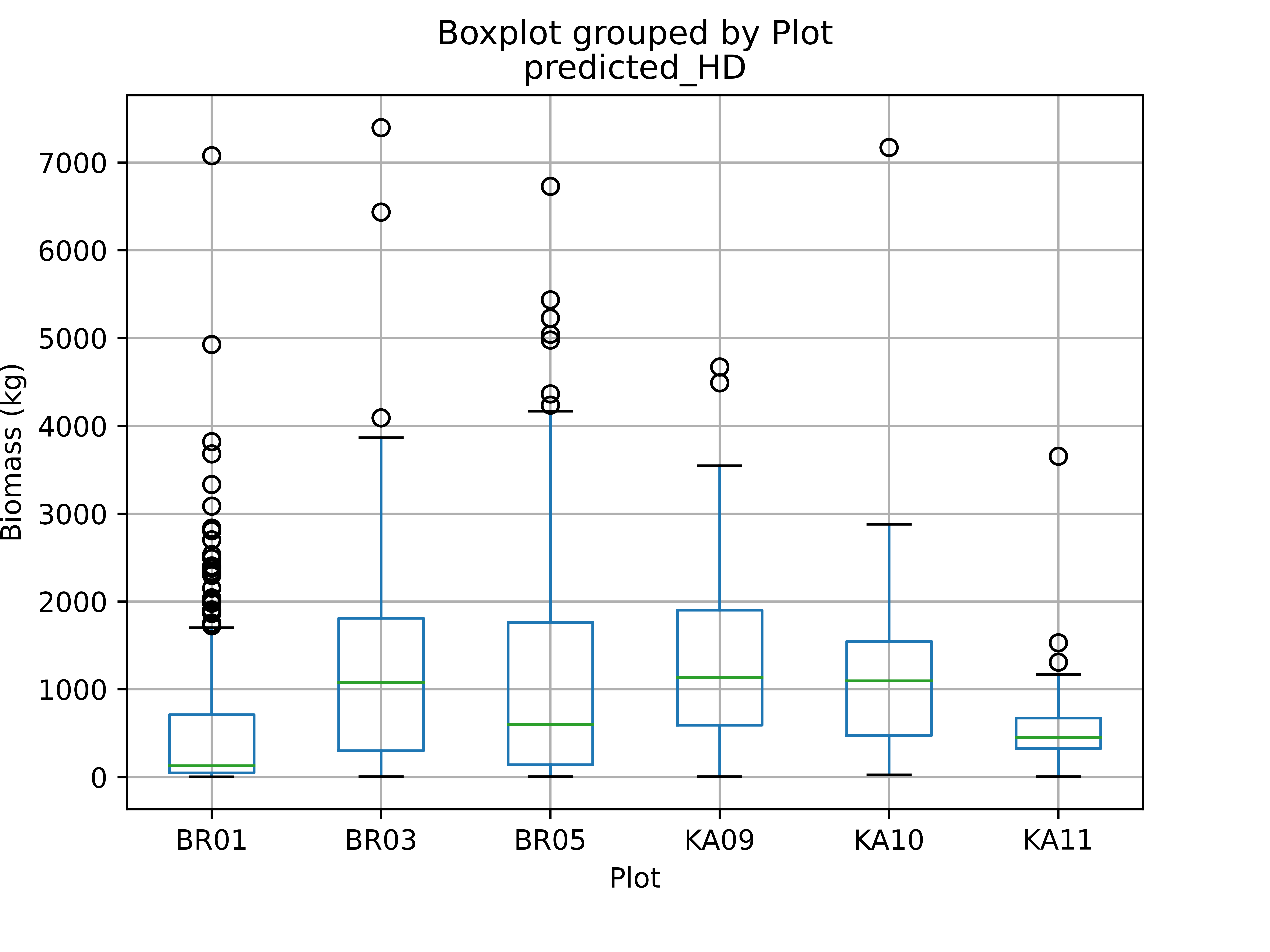
For each tree, its height, diameter, and crown diameter are derived either by field measurements and LiDAR point cloud data, and discard from the analysis trees without field measurements. For a single tree, there may exist multiple LiDAR measurements and the number of measurements fluctuates from plot to plot. Therefore, we average all measurements. Note that these measurements are incomplete, for example, tree heights were not inventoried (or measured by LiDAR data). In those cases, LiDAR-measured (or inventoried) variables were used instead. In Figure 11 (a), we present box plots of the tree biomass grouped by stands where it is indicated the following biomass statistics from bottom to top: minimum, first quartile, median, third quartile, and maximum. Outliers get represented by black, empty circles. The tree biomass value dominantly varies from zero to two Mg. Its distributions exhibit distinct characteristics for each plot. We note that the fluctuating number of outliers has the potential to impact model uncertainty.
The computation serves as a basis to compare three candidate models: LR from Equation 20 trained on Jucker data, and models RF & GPR trained on the data curated in Section IV-B. In order to derive stand-level biomass estimates, we sum up the values of individual trees. This way, the over- and underestimation of biomass, in large parts, cancel. For each plot Figure 11 (b) presents the resulting RE values of the three models RF, GPR, and LR. RF most poorly performs for all plots except KA09. However, LR underestimates the biomass in seven out of nine plots, thus there is a significant bias for errors to accumulate. In Table III we compute the relative error of the three models given all reference data. We notice the LR model rendering more biased compared with the GPR. The scatter plot in Figure 11 (c) supports that LR tends to over- and underestimate tree biomass when assuming values less and larger than 500 kg, respectively. GPR-predicted biomass estimates well correlate with the predicted biomass of the LR3 model reference.
As listed in Table III, the relative RMSE of models LR, RF, and GPR assume values 16.93%, 46.08%, and 24.46%, respectively. Although GPR is less accurate compared with the LR model, the relative RMSE of GPR is acceptable when referenced to the state-of-the-art biomass estimation errors on a national and global scale, cf. [1] quoting %RMSE values in 37% to 67%.


| LR | RF | GPR | |
|---|---|---|---|
| RE | 0.0677 | -0.1712 | 0.0021 |
| %RMSE | 0.1693 | 0.4608 | 0.2446 |
VI Conclusion
We proposed a Gaussian process regressor model to estimate biomass on individual tree level taking tree height as input, only. It enables rapid regional-to-national above-ground biomass evaluation from high-resolution LiDAR data. As a single input parameter model, a series of existing allometry databases contribute to model training. We benchmarked GPR against four established biomass models training on Jucker data and a dataset curated by this work. Results confirm GPR performs best when compared with two biomass-height models, and it achieves reasonable results in reference to a biomass-height-crown diameter model. GPR generates a low fitting uncertainty of 4.50%. Stand-level uncertainty analysis of GPR yielded an averaged relative root mean square error of 24.46%. Moreover, GPR renders less biased at a mean relative error of 0.0021. Future work may explore a stratified approach where biome-specific models [21] have the potential to decrease model uncertainty.
References
- [1] P. Rodríguez-Veiga, S. Quegan, J. Carreiras, H. J. Persson, J. E. Fransson, A. Hoscilo, D. Ziółkowski, K. Stereńczak, S. Lohberger, M. Stängel, et al., “Forest biomass retrieval approaches from earth observation in different biomes,” International Journal of Applied Earth Observation and Geoinformation, vol. 77, pp. 53–68, 2019.
- [2] “Eip-agri workshop new value chains from multifunctional forests,” Tech. Rep. 1-10, The European Innovation Partnership Agricultural Productivity and Sustainability (EIP-AGRI), Nov 2016.
- [3] Z. Xiong, F. Zhang, Y. Wang, Y. Shi, and X. X. Zhu, “EarthNets: Empowering AI in Earth Observation,” arXiv preprint arXiv:2210.04936, 2022.
- [4] M. Singh and X. X. Zhu, “Analysis of how the spatial and temporal patterns of fire and their bioclimatic and anthropogenic drivers vary across the amazon rainforest in el niño and non-el niño years,” PeerJ, vol. 9, p. e12029, 2021.
- [5] L. Duncanson, J. Armston, M. Disney, V. Avitabile, N. Barbier, K. Calders, S. Carter, J. Chave, M. Herold, N. MacBean, et al., “Aboveground woody biomass product validation good practices protocol.,” 2021.
- [6] Y. Malhi, D. Wood, T. R. Baker, J. Wright, O. L. Phillips, T. Cochrane, P. Meir, J. Chave, S. Almeida, L. Arroyo, et al., “The regional variation of aboveground live biomass in old-growth amazonian forests,” Global Change Biology, vol. 12, no. 7, pp. 1107–1138, 2006.
- [7] Y. Pan, R. A. Birdsey, J. Fang, R. Houghton, P. E. Kauppi, W. A. Kurz, O. L. Phillips, A. Shvidenko, S. L. Lewis, J. G. Canadell, et al., “A large and persistent carbon sink in the world’s forests,” Science, vol. 333, no. 6045, pp. 988–993, 2011.
- [8] J. Chave, M. Réjou-Méchain, A. Búrquez, E. Chidumayo, M. S. Colgan, W. B. Delitti, A. Duque, T. Eid, P. M. Fearnside, R. C. Goodman, et al., “Improved allometric models to estimate the aboveground biomass of tropical trees,” Global change biology, vol. 20, no. 10, pp. 3177–3190, 2014.
- [9] K. J. Anderson-Teixeira, S. J. Davies, A. C. Bennett, E. B. Gonzalez-Akre, H. C. Muller-Landau, S. Joseph Wright, K. Abu Salim, A. M. Almeyda Zambrano, A. Alonso, J. L. Baltzer, et al., “Ctfs-forest geo: a worldwide network monitoring forests in an era of global change,” Global change biology, vol. 21, no. 2, pp. 528–549, 2015.
- [10] Y. Luo, X. Wang, Z. Ouyang, F. Lu, L. Feng, and J. Tao, “A review of biomass equations for china’s tree species,” Earth System Science Data, vol. 12, no. 1, pp. 21–40, 2020.
- [11] H. Carreno-Luengo, G. Luzi, and M. Crosetto, “Above-ground biomass retrieval over tropical forests: A novel gnss-r approach with cygnss,” Remote Sensing, vol. 12, no. 9, p. 1368, 2020.
- [12] M. Santoro, C. Beer, O. Cartus, C. Schmullius, A. Shvidenko, I. McCallum, U. Wegmüller, and A. Wiesmann, “Retrieval of growing stock volume in boreal forest using hyper-temporal series of envisat asar scansar backscatter measurements,” Remote Sensing of Environment, vol. 115, no. 2, pp. 490–507, 2011.
- [13] M. Hayashi, T. Motohka, and Y. Sawada, “Aboveground biomass mapping using alos-2/palsar-2 time-series images for borneo’s forest,” IEEE Journal of Selected Topics in Applied Earth Observations and Remote Sensing, vol. 12, no. 12, pp. 5167–5177, 2019.
- [14] M. Schlund, S. Erasmi, and K. Scipal, “Comparison of aboveground biomass estimation from insar and lidar canopy height models in tropical forests,” IEEE Geoscience and Remote Sensing Letters, vol. 17, no. 3, pp. 367–371, 2019.
- [15] P. L. Patterson, S. P. Healey, G. Ståhl, S. Saarela, S. Holm, H.-E. Andersen, R. O. Dubayah, L. Duncanson, S. Hancock, J. Armston, et al., “Statistical properties of hybrid estimators proposed for gedi—nasa’s global ecosystem dynamics investigation,” Environmental Research Letters, vol. 14, no. 6, p. 065007, 2019.
- [16] C. A. Silva, L. Duncanson, S. Hancock, A. Neuenschwander, N. Thomas, M. Hofton, L. Fatoyinbo, M. Simard, C. Z. Marshak, J. Armston, et al., “Fusing simulated gedi, icesat-2 and nisar data for regional aboveground biomass mapping,” Remote Sensing of Environment, vol. 253, p. 112234, 2021.
- [17] F. Banda, D. Giudici, T. Le Toan, M. Mariotti d’Alessandro, K. Papathanassiou, S. Quegan, G. Riembauer, K. Scipal, M. Soja, S. Tebaldini, et al., “The biomass level 2 prototype processor: Design and experimental results of above-ground biomass estimation,” Remote Sensing, vol. 12, no. 6, p. 985, 2020.
- [18] S. Ganz, Y. Käber, and P. Adler, “Measuring tree height with remote sensing—a comparison of photogrammetric and lidar data with different field measurements,” Forests, vol. 10, no. 8, p. 694, 2019.
- [19] W. Yao, P. Krzystek, and M. Heurich, “Tree species classification and estimation of stem volume and dbh based on single tree extraction by exploiting airborne full-waveform lidar data,” Remote Sensing of Environment, vol. 123, pp. 368–380, 2012.
- [20] L. Duncanson, B. Cook, G. Hurtt, and R. Dubayah, “An efficient, multi-layered crown delineation algorithm for mapping individual tree structure across multiple ecosystems,” Remote Sensing of Environment, vol. 154, pp. 378–386, 2014.
- [21] T. Jucker, J. Caspersen, J. Chave, C. Antin, N. Barbier, F. Bongers, M. Dalponte, K. Y. van Ewijk, D. I. Forrester, M. Haeni, et al., “Allometric equations for integrating remote sensing imagery into forest monitoring programmes,” Global change biology, vol. 23, no. 1, pp. 177–190, 2017.
- [22] L. J. Klein, W. Zhou, and C. M. Albrecht, “Quantification of carbon sequestration in urban forests,” workshop on Tackling Climate Change with Machine Learning at ICML2021, arXiv:2106.00182, 2021.
- [23] G. P. Asner and J. Mascaro, “Mapping tropical forest carbon: Calibrating plot estimates to a simple lidar metric,” Remote Sensing of Environment, vol. 140, pp. 614–624, 2014.
- [24] G. P. Asner, D. E. Knapp, R. E. Martin, R. Tupayachi, C. B. Anderson, J. Mascaro, F. Sinca, K. D. Chadwick, M. Higgins, W. Farfan, et al., “Targeted carbon conservation at national scales with high-resolution monitoring,” Proceedings of the National Academy of Sciences, vol. 111, no. 47, pp. E5016–E5022, 2014.
- [25] I. Shendryk, M. Broich, M. G. Tulbure, and S. V. Alexandrov, “Bottom-up delineation of individual trees from full-waveform airborne laser scans in a structurally complex eucalypt forest,” Remote Sensing of Environment, vol. 173, pp. 69–83, 2016.
- [26] D. Panagiotidis, A. Abdollahnejad, P. Surovỳ, and V. Chiteculo, “Determining tree height and crown diameter from high-resolution uav imagery,” International journal of remote sensing, vol. 38, no. 8-10, pp. 2392–2410, 2017.
- [27] H. Weiser, J. Schäfer, L. Winiwarter, N. Krašovec, C. Seitz, M. Schimka, K. Anders, D. Baete, A. S. Braz, J. Brand, D. Debroize, P. Kuss, L. L. Martin, A. Mayer, T. Schrempp, L.-M. Schwarz, V. Ulrich, F. E. Fassnacht, and B. Höfle, “Terrestrial, UAV-borne, and airborne laser scanning point clouds of central European forest plots, Germany, with extracted individual trees and manual forest inventory measurements,” 2021.
- [28] T. Mette, I. Hajnsek, and K. Papathanassiou, “Height-biomass allometry in temperate forests performance accuracy of height-biomass allometry,” in IGARSS 2003. 2003 IEEE International Geoscience and Remote Sensing Symposium. Proceedings (IEEE Cat. No. 03CH37477), vol. 3, pp. 1942–1944, IEEE, 2003.
- [29] A. T. Caicoya, F. Kugler, I. Hajnsek, and K. P. Papathanassiou, “Large-scale biomass classification in boreal forests with tandem-x data,” IEEE Transactions on Geoscience and Remote Sensing, vol. 54, no. 10, pp. 5935–5951, 2016.
- [30] C. Choi, M. Pardini, M. Heym, and K. P. Papathanassiou, “Improving forest height-to-biomass allometry with structure information: A tandem-x study,” IEEE Journal of Selected Topics in Applied Earth Observations and Remote Sensing, vol. 14, pp. 10415–10427, 2021.
- [31] S. Solberg, E. H. Hansen, T. Gobakken, E. Naessset, and E. Zahabu, “Biomass and insar height relationship in a dense tropical forest,” Remote Sensing of Environment, vol. 192, pp. 166–175, 2017.
- [32] M. J. Sullivan, S. L. Lewis, W. Hubau, L. Qie, T. R. Baker, L. F. Banin, J. Chave, A. Cuni-Sanchez, T. R. Feldpausch, G. Lopez-Gonzalez, et al., “Field methods for sampling tree height for tropical forest biomass estimation,” Methods in Ecology and Evolution, vol. 9, no. 5, pp. 1179–1189, 2018.
- [33] R. E. McRoberts and J. A. Westfall, “Propagating uncertainty through individual tree volume model predictions to large-area volume estimates,” Annals of Forest Science, vol. 73, pp. 625–633, 9 2016.
- [34] C. M. Albrecht, F. J. Marianno, and L. J. Klein, “Autogeolabel: Automated label generation for geospatial machine learning,” IEEE BigData2021 conference, in press, 2021.
- [35] L. J. Klein, F. J. Marianno, C. M. Albrecht, M. Freitag, S. Lu, N. Hinds, X. Shao, S. B. Rodriguez, and H. F. Hamann, “Pairs: A scalable geo-spatial data analytics platform,” in 2015 IEEE International Conference on Big Data (Big Data), pp. 1290–1298, IEEE, 2015.
- [36] D. S. Falster, R. A. Duursma, M. I. Ishihara, D. R. Barneche, R. G. FitzJohn, A. Vårhammar, M. Aiba, M. Ando, N. Anten, M. J. Aspinwall, et al., “Baad: A biomass and allometry database for woody plants.,” tech. rep., Ecological Society of America, 2015.
- [37] V. A. Usoltsev, “Sample tree biomass data for eurasian forests,” 2015.
- [38] D. M. Olson, E. Dinerstein, E. D. Wikramanayake, N. D. Burgess, G. V. Powell, E. C. Underwood, J. A. D’amico, I. Itoua, H. E. Strand, J. C. Morrison, et al., “Terrestrial ecoregions of the world: A new map of life on eartha new global map of terrestrial ecoregions provides an innovative tool for conserving biodiversity,” BioScience, vol. 51, no. 11, pp. 933–938, 2001.
- [39] J. Stewart, A. Dunsdon, J. Hellin, and C. Hughes, Wood biomass estimation of Central American dry zone species. Oxford Forestry Institute, University of Oxford, 1992.
- [40] Q. M. Ketterings, R. Coe, M. van Noordwijk, C. A. Palm, et al., “Reducing uncertainty in the use of allometric biomass equations for predicting above-ground tree biomass in mixed secondary forests,” Forest Ecology and management, vol. 146, no. 1-3, pp. 199–209, 2001.
- [41] T. Basuki, P. Van Laake, A. Skidmore, and Y. Hussin, “Allometric equations for estimating the above-ground biomass in tropical lowland dipterocarp forests,” Forest ecology and management, vol. 257, no. 8, pp. 1684–1694, 2009.
- [42] S. I. Maulana, Y. Wibisono, and S. Utomo, “Development of local allometric equation to estimate total aboveground biomass in papua tropical forest,” Indonesian Journal of Forestry Research, vol. 3, no. 2, pp. 107–118, 2016.
- [43] X. Zhou and M. A. Hemstrom, “Estimating aboveground tree biomass on forest land in the pacific northwest: a comparison of approaches,” Res. Pap. PNW-RP-584. Portland, OR: US Department of Agriculture, Forest Service, Pacific Northwest Research Station. 18 p., vol. 584, 2009.
- [44] L. Isserlis, “On a formula for the product-moment coefficient of any order of a normal frequency distribution in any number of variables,” Biometrika, vol. 12, no. 1/2, pp. 134–139, 1918.
- [45] C. M. Bishop and N. M. Nasrabadi, Pattern recognition and machine learning. Springer, 2006.
- [46] R. Bellman, Introduction to matrix analysis. SIAM, 1997.
- [47] C. Williams and C. Rasmussen, “Gaussian processes for regression,” Advances in neural information processing systems, vol. 8, 1995.
- [48] G. Camps-Valls, L. Martino, D. H. Svendsen, M. Campos-Taberner, J. Muñoz-Marí, V. Laparra, D. Luengo, and F. J. García-Haro, “Physics-aware gaussian processes in remote sensing,” Applied Soft Computing, vol. 68, pp. 69–82, 2018.
- [49] Z. Xiong, H. Li, and X. X. Zhu, “Doubly deformable aggregation of covariance matrices for few-shot segmentation,” in Computer Vision–ECCV 2022: 17th European Conference, Tel Aviv, Israel, October 23–27, 2022, Proceedings, Part XX, pp. 133–150, Springer, 2022.
![[Uncaptioned image]](2305.09555v2/QianSong3.jpg) |
Qian Song (S’16-M’20) received the B.E. degree (Hons.) from the School of Information Science and Technology, East China Normal University, Shanghai, China, in 2015, and the Ph.D. degree (Hons.) from Fudan University, Shanghai, China, in 2020. She was a post-doctoral fellow with the Remote Sensing Technology Institute (IMF), German Aerospace Center (DLR), Wessling, Germany from 2020 to 2022. Since 2023, she is a post-doctoral fellow with the Chair of Data Science in Earth Observation at the Technical University of Munich (TUM), Munich, Germany. She has been awarded as the URSI (International Union of Radio Science) Young Scientist Award in 2020. Her research interests include advanced deep learning technologies and their applications in synthetic aperture radar image interpretation, forest monitoring and biomass estimation. |
![[Uncaptioned image]](2305.09555v2/Albrecht_2020.jpg) |
Conrad M Albrecht (M’17) received an undergraduate degree in physics from Technical University Dresden, Germany, in 2007 and a Ph.D. degree in physics with an extra certification in computer science from Heidelberg University, Germany, in 2014. Spanning the fields of physics, mathematics, and computer science, among others, he was a visiting scientist with CERN, Switzerland, in 2010, and with the Dresden Max Planck Institute for the Physics of Complex Systems, Germany, in 2007. In 2015 Conrad became a research scientist with the IBM T.J. Watson Research Center, Yorktown Heights, NY, USA. Currently, since April 2021, he leads a HelmholtzAI-funded team for ”Large-Scale Data Mining in Earth Observation” (DM4EO) at the German Aerospace Center, Oberpfaffenhofen, Germany in close collaboration with Technical University Munich. Starting 2023, Conrad’s team contributes to Horizon Europe project EvoLand, https://www.evo-land.eu. Conrad’s research agenda interconnects physical models and numerical analysis, employing Big Data technologies and machine learning. As part of the ”Data Intensive Physical Analytics” team in IBM Research, he significantly contributed to industry-level solutions processing geospatial information with focus on machine-learning driven remote sensing applications. He co-organized workshops at the IEEE BigData conference, the EGU General Assembly, and the AAAS annual meeting. Home to the US and the EU, Conrad’s scientific agenda aims to strengthen transatlantic collaboration of corporate research and academia. His DM4EO team collaborates with institutions such as Juelich Super-Computing Center, GFZ German Research Centre for Geosciences, INRIA Grenoble, Princeton University, IBM Research, and Yale University. |
![[Uncaptioned image]](2305.09555v2/Zhitong_Xiong.png) |
Zhitong Xiong received the Ph.D. degree in computer science and technology from Northwestern Polytechnical University, Xi’an, China, in 2021. He is currently a senior scientist and leads the ML4Earth working group with the Data Science in Earth Observation, Technical University of Munich (TUM), Germany. His research interests include computer vision, machine learning, Earth observation, and Earth system modeling. |
![[Uncaptioned image]](2305.09555v2/Xiao_Xiang_Zhu.png) |
Xiao Xiang Zhu (S’10–M’12–SM’14–F’21) received the Master (M.Sc.) degree, her doctor of engineering (Dr.-Ing.) degree and her “Habilitation” in the field of signal processing from Technical University of Munich (TUM), Munich, Germany, in 2008, 2011 and 2013, respectively. She is the Chair Professor for Data Science in Earth Observation at TUM and was the founding Head of the Department “EO Data Science” at the Remote Sensing Technology Institute, German Aerospace Center (DLR). Since 2019, Zhu is a co-coordinator of the Munich Data Science Research School (www.mu-ds.de). Since 2019 She also heads the Helmholtz Artificial Intelligence – Research Field “Aeronautics, Space and Transport”. Since May 2020, she is the PI and director of the international future AI lab ”AI4EO – Artificial Intelligence for Earth Observation: Reasoning, Uncertainties, Ethics and Beyond”, Munich, Germany. Since October 2020, she also serves as a Director of the Munich Data Science Institute (MDSI), TUM. Prof. Zhu was a guest scientist or visiting professor at the Italian National Research Council (CNR-IREA), Naples, Italy, Fudan University, Shanghai, China, the University of Tokyo, Tokyo, Japan and University of California, Los Angeles, United States in 2009, 2014, 2015 and 2016, respectively. She is currently a visiting AI professor at ESA’s Phi-lab. Her main research interests are remote sensing and Earth observation, signal processing, machine learning and data science, with their applications in tackling societal grand challenges, e.g. Global Urbanization, UN’s SDGs and Climate Change. Dr. Zhu is a member of young academy (Junge Akademie/Junges Kolleg) at the Berlin-Brandenburg Academy of Sciences and Humanities and the German National Academy of Sciences Leopoldina and the Bavarian Academy of Sciences and Humanities. She serves in the scientific advisory board in several research organizations, among others the German Research Center for Geosciences (GFZ) and Potsdam Institute for Climate Impact Research (PIK). She is an associate Editor of IEEE Transactions on Geoscience and Remote Sensing and serves as the area editor responsible for special issues of IEEE Signal Processing Magazine. She is a Fellow of IEEE. |