Probing massive black holes with gravitational waves2022Probing massive black holes with gravitational waves–11
Abstract
We investigate the coalescence of massive black hole () binaries (MBHBs) at by adopting a suite of cosmological hydrodynamical simulations of galaxy formation, zoomed-in on biased () overdense regions ( dark matter halos at ) of the Universe. We first analyse the impact of different resolutions and AGN feedback prescriptions on the merger rate, assuming instantaneous mergers. Then, we compute the halo bias correction factor due to the overdense simulated region. Our simulations predict merger rates that range between 3 – 15 at , depending on the run considered, and after correcting for a bias factor of .
For our fiducial model, we further consider the effect of delay in the MBHB coalescence due to dynamical friction. We find that 83 per cent of MBHBs will merge within the Hubble time, and 21 per cent within 1 Gyr, namely the age of the Universe at . We finally compute the expected properties of the gravitational wave (GW) signals and find the fraction of LISA detectable events with high signal-to-noise ratio (SNR 5) to range between 66-69 per cent. However, identifying the electro-magnetic counterpart of these events remains challenging due to the poor LISA sky localization that, for the loudest signals ( at ), is around 10 .
Keywords:
Supermassive black holes – gravitational waves – galaxies: high-redshift1 Introduction
It is now widely agreed that that the centres of nearby galaxies host massive black holes (MBHs, ) whose masses correlates with several properties of the host galaxy itself (Magorrian et al. 1998; Kormendy 2001, e.g.). Observational evidences also indicate the existence of bright quasars at (e.g. Fan et al. 2006; Jiang et al. 2010) powered by super massive black holes (SMBHs, ) that are accreting close to the Eddington rate. It is still a theoretical challenge to explain how such SMBHs have been assembled within 1 Gyr after the birth of the Universe.
These bright, high- quasars are expected to be located in massive dark matter (DM) halos (). According to the hierarchical structure formation scenario (e.g. White & Rees 1978; Peebles 1980; Blumenthal et al. 1984), such massive DM halos result from the mergers of smaller halos that formerly harboured the initial seeds of the SMBHs we observe at . Several candidates have been proposed so far as SMBH seeds: (i) light seeds (), formed as remnants of Pop III stars (Madau et al. 1998; Heger et al. 2003; Yoshida et al. 2008; Hirano et al. 2015) at ; (ii) intermediate seeds (), produced in compact nuclear star clusters as a consequence of runaway stellar mergers at (Davies et al. 2011; Devecchi et al. 2012; Lupi et al. 2014; Mapelli 2016; Reinoso et al. 2018); (iii) heavy seeds or direct collapse black holes (DCBHs, ), resulting from the rapid collapse of metal poor gas clouds in atomic cooling halos (virial temperature ) where star formation is prevented by intense H2 photo-dissociating Lyman Werner (LW) radiation (Haehnelt 1994; Loeb & Rasio 1994; Eisenstein & Loeb 1995; Silk & Rees 1998; Shang et al. 2010; Johnson et al. 2012; Yue et al. 2013; Ferrara et al. 2014).
Numerous uncertainties remain associated to each of the scenarios discussed above (e.g.Volonteri et al. 2003; Koushiappas et al. 2004; Begelman et al. 2006; Lodato & Natarajan 2006; Volonteri & Bellovary 2012; Tanaka & Haiman 2009; Latif et al. 2013; Woods et al. 2019). To understand which of the aforementioned scenarios is the most promising in order to explain the presence of SMBHs at it is necessary to study the still undiscovered population of Intermediate-Mass black holes (IMBHs, ) at . Various works have investigated the possibility that these IMBHs lie at the centers of dwarf galaxies (Reines et al. 2013; Silk 2017; Barai & de Gouveia Dal Pino 2019), and it is difficult to detect them at high-z because of low surface brightness of the galaxies as well as the low intensity of the IMBHs.
The proposed space-borne GW observatory Laser Interferometer Space Antennae (LISA; eLISA Consortium et al. 2013), due to be launched in 2034, is potentially an exquisite tool to accomplish this goal. LISA is in fact designed to be sensitive to signals in the frequency range Hz, thus capable to detect GWs from massive () BH binaries at very-high redshift (Haehnelt 1994; Jaffe & Backer 2003; Wyithe & Loeb 2003; Sesana et al. 2004; Sesana et al. 2005; Amaro-Seoane et al. 2022, even if BHs in this mass range already exist at such early epochs;). Different scenarios of BH seeds are expected to leave signatures in all those observables that can be probed by GW observations of MBHBs (Bhowmick et al. 2022, e.g. merger rates, BH mass distribution;).
Several studies have used semi-analytical models to estimate the MBHB merger rate. For instance, Sesana et al. 2007 made predictions for the merger rate of MBHs when the compact objects start their evolution either as DCBHs or as Pop III star remnants. In this study, the authors considered different stellar feedback regimes to trace the metal enrichment in the gas halos of MBH formation. Differently, Hartwig et al. 2018 quantified the rate of in-situ mergers from binaries of DCBHs. Dayal et al. 2019 investigated the dependence of the merger rate on the seed mass (light versus heavy seeds), the merger prescription (instantaneous versus delayed merger), and cosmic reionization. Barausse et al. 2020 focussed on different seeding models, including various astrophysical processes, such as supernovae feedback. Comparably, numerous semi-analytical models, such as Begelman et al. 2006; Arun et al. 2009; Klein et al. 2016; Bonetti et al. 2019; Valiante et al. 2020, explored different evolutionary channels of MBHB formation (seed mass, accretion efficiency, metal enrichment, merger timescales) that could be detected by milli-Hz GW facilities, like LISA.
A different approach instead takes advantage of cosmological hydrodynamical simulations (Di Matteo et al. 2012; Vogelsberger et al. 2014; Schaye et al. 2015; Volonteri et al. 2017, e.g.) to study the dynamics of gas and its effect on the evolution of high redshift quasars. Salcido et al. 2016 studied the SMBH mergers occurring in a fully cosmological simulation. In particular, the authors looked for the expected LISA detection rate in the EAGLE run (Schaye et al. 2015), including also a prescription to delay the mergers. More recently, several works made predictions for the LISA detection rate taking advantage of the Illustris simulations (Nelson et al. 2015). Particularly, Katz et al. 2019 analysed the effect of different evolutionary models for MBHB and studied the detectability of the merger events (Katz & Larson 2019, see also). DeGraf & Sijacki 2019 studied how different seeding models can affect the statistical properties of the MBH population, and the resulting merger rate. Furthermore, DeGraf et al. 2021 explored the relation between SMBH mergers and the morphology of their host galaxies at .
In this work, we adopt cosmological zoom-in hydrodynamical simulations of galaxy formation, based on the GADGET-3 code, to investigate the coalescence of massive black hole () binaries at . We consider a suite of simulations which differ both in terms of resolution and in the stellar/AGN feedback prescriptions implemented and investigate the impact of resolution and feedback on the merger rates of massive black hole binaries. For our fiducial model, we further investigate the associated GW properties (chirp mass, merger rate, characteristic strain, signal-to-noise ratio, angular resolution) of the MBHBs. We also quantify the effect of considering delays in MBHB merging due to dynamical friction on such GW properties. The paper is organized as follows: in Section 2, we describe the numerical simulations analysed in this work; in Section 3, we study the merger rate resulting from our simulations and in Section 4 we analyse the effect of adding delays in the MBHB coalescence in post-processing. In Section 5 we analyze the GW properties from the MBHB mergers. Finally, we discuss our results in Section 6 and draw our conclusions in Section 7.
2 Simulations
In this section, we describe the cosmological hydrodynamical simulations adopted in this work. We select simulations from the suites introduced by Valentini et al. 2021 – hereafter 106 – and Barai et al. 2018 – hereafter 5.
The simulations are performed with the TreePM (particle mesh) + SPH (Smoothed Particles Hydrodynamics) code gadget-3, an evolution of the public gadget-2 code (Springel 2005), and follow the evolution of a M⊙ halo at . In particular, we consider the following runs from 106:
-
AGN_fid: our fiducial model, featuring thermal AGN feedback;
-
BHs_noFB: a control run, analogous to AGN_fid, in which BHs and their accretion are included, but AGN feedback is turned off;
and the following runs from 5:
-
AGNcone: in which the kinetic feedback is distributed in a bi-cone with and half-opening angle of °.
-
AGNsphere: featuring isotropic, kinetic AGN feedback;
We summarise in the following sections the other main features of the simulations that are relevant for the present study, while we refer to the aforementioned papers for details.
2.1 Valentini et al. 2021 models: AGN_fid and BHs_noFB
2.1.1 Initial conditions and resolution
The initial conditions are generated with the code music11 1 music–Multiscale Initial Conditions for Cosmological Simulations: https://bitbucket.org/ohahn/music. (Hahn & Abel 2011), assuming a CDM cosmology22 2 We adopt the following parameters by the Planck Collaboration et al. 2016: , , , .. First, a dark matter (DM)-only simulation is run from to , with DM particles having a mass of in a comoving volume of . Then, a halo as massive as at is selected for a zoom-in procedure, to run the full hydrodynamical simulation. In the zoom-in region, the highest resolution particles have a mass of and . The gravitational softening lengths are33 3 We use the following convention when indicating distances: a letter c before the corresponding unit refers to comoving distances (e.g. ckpc), while the letter p refers to physical units (e.g. pkpc). When not explicitly stated, we are referring to physical distances. ckpc and ckpc for DM and baryon particles, respectively.
| AGN_fid | BHs_noFB | AGNcone | AGNsphere | |||||||||||||||||||
| z=6 |
|
| ||||||||||||||||||||
| [] | ||||||||||||||||||||||
|
200 | 190 | 200 | 300 | ||||||||||||||||||
|
|
||||||||||||||||||||||
|
35 | 89 | 3 | |||||||||||||||||||
| Feedback | Stellar, AGN(thermal) | Stellar |
|
| ||||||||||||||||||
2.1.2 Sub-resolution physics
-
Cooling, star formation and stellar feedback: the multiphase interstellar medium (ISM) is described by means of the MUlti Phase Particle Integrator (MUPPI) sub-resolution model (Murante et al. 2010; Murante et al. 2015; Valentini et al. 2017; Valentini et al. 2019). It features metal lines cooling, an -based star formation, thermal and kinetic stellar feedback, the presence of an UV background, and the Tornatore et al. 2007 model for chemical evolution.
-
Black holes seeding and merging: BHs are treated as collisionless sink particles. Seeds of mass are implanted in DM halos with mass exceeding . This seeding prescription is meant to mimic in a simplistic way the DCBH scenario described in the 1 Introduction section. Two BHs are allowed to merge when their relative distance becomes smaller than twice the BH gravitational softening length, and their relative velocity is lower than the sound speed of the local ISM. The final BH is set on the position of the most massive BH which underwent the merger. BH repositioning (or pinning) is implemented, in order to prevent BHs from wandering from the centre of the halo in which they reside: at each time-step BHs are shifted towards the position of minimum gravitational potential within their softening length (Booth & Schaye 2009; Schaye et al. 2015; Weinberger et al. 2017; Pillepich et al. 2018, as also done in e.g.).
-
Gas accretion on BHs: besides BH-BH mergers, black holes are also allowed to grow via gas accretion, as described by the classical Bondi-Hoyle-Lyttleton (BHL) model (Hoyle & Lyttleton 1939; Bondi & Hoyle 1944; Bondi 1952; Edgar 2004):
(1) where is the gravitational constant, is the BH mass, is the gas density, is the sound speed, and is the velocity of the BH relative to the gas. These quantities are evaluated by averaging over the SPH gas particles within the BH smoothing length, with kernel-weighted contributions. Eq. 1 is used to estimate the contribution to the accretion rate from the cold and hot phase of the ISM, separately (Steinborn et al. 2015; Valentini et al. 2020). Accretion from the cold gas is reduced by taking into account its angular momentum (see Valentini et al. 2020, for details). The BH accretion rate is capped to the Eddington accretion rate.
-
Quasar feedback: a fraction of the accreted rest-mass energy is radiated away with a radiative efficiency , thereby providing a bolometric luminosity for an accreting BH equals to:
(2) where is the speed of light and (Sądowski & Gaspari 2017). Then, a fraction (106) of the radiated luminosity is coupled thermally and isotropically to the gas surrounding the BH. The AGN feedback energy is distributed to the hot and cold phases of the multiphase gas particles within the BH smoothing volume (Valentini et al. 2020).
2.2 Barai et al. 2018 simulations: AGNcone and AGNsphere
2.2.1 Initial conditions and resolution
Initial conditions are generated as in 106 with the code music and adopting the same cosmology. The parent, DM-only simulation follows a comoving volume of , with DM particles having . The zoom-in run focuses on a DM halo as massive as ; the highest resolution particles have and , with a gravitational softening length ckpc.
2.2.2 Sub-resolution physics
-
Cooling, star formation and stellar feedback: radiative heating and cooling is accounted for by employing the CLOUDY cooling tables computed by Wiersma et al. 2009. Star formation is implemented following the ISM multiphase model by Springel & Hernquist 2003, in which an hot and a cold phase co-exist in pressure equilibrium, and assuming a density threshold for the star formation of . A Chabrier 2003 initial mass function (IMF) in the mass range is adopted. Stellar evolution and chemical enrichment are computed following Tornatore et al. 2007.
-
Black hole seeding and merging: As in 5, the theoretical mass of seed BHs is . However, their dynamical mass is much smaller in the 106 simulations ( in 106 versus in 5). The prescription is in fact more refined in 106, where seeded BHs are linked to stellar particles instead of DM particles. We further discuss this point in Sec. 3.1.
-
Gas accretion on BHs: as in 106, the BHL model is adopted. However, the lower resolution of the 5 simulations does not allow to properly describe the accretion process: thus Eq. 1 is multiplied by a numerical boost factor (Springel et al. 2005; Sijacki et al. 2009; Vogelsberger et al. 2014). No angular momentum effects are included in the 5 formalism, and no distinction between the hot and cold gas phases is considered.
-
Quasar feedback: black holes are assumed to radiate energy away with an efficiency of , and a fraction of this energy is coupled to the surrounding gas via kinetic feedback as an energy-driven wind (see Barai et al. 2018 for details). The geometry of the feedback is bi-conical (i.e. energy is injected onto a bi-cone with a half-opening angle of °) in AGNcone and spherical (i.e. energy distributed isotropically) in AGNsphere. BHs grow times more massive at in the AGNcone case than in the AGNsphere run as shown in top panels of fig: 2 in 5. This is because in the AGNcone run more gas can inflow along the perpendicular direction to the bi-cone, and accrete onto the black hole.
A summary of the two different simulation models are provided in Table 1 for a comprehensive view.
3 Merger rate
3.1 Merger rate from overdense regions
For the models summarised in Tab. 1, we compute the redshift evolution of the MBH merger rate (per unit redshift, per unit time) for different chirp mass ranges, where the chirp mass is given by ( e.g. Cutler & Flanagan 1994; Blanchet et al. 1995):
| (3) |
and and are the masses of the merging black holes44 4 In these calculations, we do not include those MBHBs that cannot be associated with any galaxy in the simulations. We discuss these spurious events in Sec. 4.1. We show in Fig. 1 the normalized probability distribution function (PDF) of the chirp masses resulting from different simulations. Although no evident differences among different models can be seen from this plot, we note that the 5 simulations predict a larger number of small chirp masses () with respect to to 106, and only the BHs_noFB and AGNcone simulations predict MBHBs with .


We then calculate the merger rate from the number density of mergers, dN/dz per comoving volume, dV as (e.g. Haehnelt 1994; Ciardi & Loeb 2000):
| (4) |
where is the luminosity distance of the event. The results are shown in Fig. 2.
The number of MBH mergers predicted by our zoom-in cosmological simulations increases with decreasing redshift, as a consequence of the hierarchical structure formation process. Fig. 2 shows that the two sets of simulations have different merging histories that depend both on the numerical resolution adopted and on the feedback implemented.
In particular, Fig. 2 shows that the number of mergers predicted by the 106 simulations ( 100 at for both AGN_fid and BHs_noFB) is smaller by a factor of at least 2 than the one by the 5 simulations (>200 for both AGNcone and AGNsphere case at ). This major difference is likely linked to the better numerical resolution of the 106 simulations with respect to the 5 ones (see table 1). The condition for seeding () is more easily satisfied in 5 with respect to 106, because of the larger mass of its resolution elements. This thus implies a larger number of seeds and consequently a larger number of mergers. Even more importantly, the excess of mergers in 5 is driven by the high dynamical mass which enters in the BH-BH merger algorithm within the code.
For a fixed numerical resolution, it is possible to study the dependence of the number of mergers on the feedback implemented. In the 106 simulations, we find that for low chirp masses () the merger rate predicted by the AGN_fid model is higher than the BHs_noFB case. We further note that for this trend is reversed, the merger rate in the BHs_noFB run is higher than in the AGN_fid case. The lack of AGN feedback allows a more efficient gas accretion which makes the black holes to grow more massive and numerous in the BHs_noFB case in this particular chirp mass range.
Furthermore, we study the trend of the local sound speed in the ISM. In the left panels of Fig. 3 we show the results for the 106 simulation runs. We note that the sound speed is larger in the BHs_noFB run because of the following. In the BHs_noFB run, the accretion rate is higher than in AGN_fid (see Tab. 1); furthermore, on scales over which is computed (i.e. the smoothing length of the black holes), the heating due to accretion (gravitational compression) dominates the heating due to feedback. Thus, the gas temperature (and consequently ) in the BHs_noFB run is higher than AGN_fid. We thus conclude that for , the merger rate is driven mainly by the gravity, dynamics and substructure mergers.
For the 5 runs, we observe from Fig. 2 that in AGNcone the number of mergers is larger by a factor of 2 with respect to the AGNsphere case. To investigate this point, in the right panels of Fig. 3 we show the PDF of the relative sound speed of the merging BHs resulting from these simulations. This figure shows that in the AGNcone case, the PDF is shifted towards larger values. As discussed in Sec. 2 two BHs are allowed to merge when their relative velocity is lower than the sound speed of the local ISM. The higher is the sound speed the larger is the probability for two BHs to merge. The sound speed is larger in the AGNcone run because in this case the accretion is by far higher than in AGNsphere (see Tab. 1), resulting in a higher number of mergers.
We further note that Zana et al. 2022 already found that different feedback prescriptions result into different merger rates: in AGNcone, galaxies merge faster and more easily than in AGNsphere, possibly because of the stronger feedback due to the larger black hole accretion rate (see Tab. 1). This determines a more diffuse gas and stellar component around the host galaxies which can boost the effect of dynamical friction when two galaxies approach, thus lowering the dynamical timescale for their merging to occur.
We finally note that different resolutions and feedback prescriptions also affect the epoch at which the furthest merger event is occurring. For example, for , the furthest GW signal occurs in the redshift interval and in the case of 106 and 5 simulations, respectively.

3.2 Bias in zoom-in simulations
Our results are based on small box simulations, zoomed-in on a massive, biased (Barkana & Loeb 2001, , e.g.) dark matter halo. As a result, the number density of MBHB mergers within the simulated box overestimates the value in an average region of the Universe. In what follows, we estimate the bias of our predictions considering our fiducial run (AGN_fid).
Following the halo mass history suggested by Correa et al. 2015a, we first calculate the accreted mass () at of a halo at :
| (5) |
where and , respectively (Correa et al. 2015b). We find .
In practice, when computing the merger rate with Eq. 4, we are considering a Universe where all DM halos have and comoving volume . The result of this procedure will be clearly biased compared to a proper calculation in which DM halos span a wider mass range () and have different abundances. This bias cannot be directly computed from our simulations, but we need to rely on a semi-analytical model (SAM). In SAMs, in fact, a wide range of halos are simulated and the merger rate is computed from their collective output, by weighting each halo mass according to the Press and Schechter halo mass function (Press & Schechter 1974). This latter step is simply obtained by dividing the the merger rate by the effective comoving volume occupied by that halo. It is therefore also possible to use the SAM output to create biased universes, simply by taking halos of a desired mass and weighting them with a desired effective comoving volume. By comparing the rates obtained from this biased universe to the total one, we can infer the bias. This is the procedure we follow here.
We then use the semi-analytical model by Barausse 2012, and we consider the output of all the trees, weighted on the Press and Schechter halo mass function (Press & Schechter 1974). For these calculations, we consider the "Q3nod" run, since it is based on a model that more closely resembles our prescriptions (heavy seeds and no time delays). Furthermore, for a fair comparison with our results, we only consider merger events occurring in dark matter haloes (the threshold mass used in our simulations to seed MBHs) and involving binaries with both BH masses (the mass of our seeds). The merger rate obtained in this case is yr-1.
We next consider two specific merger trees, whose halos at are the closest to the value computed above, namely and . We weight the merger rates in these two merger trees with the inverse of the comoving volume of our refined simulation, namely (5.25 cMpc)3. The average of the two merger rates obtained in this way can be used as a proxy for the merger rate in a Universe made only of halos of at . The merger rate obtained in this case is 60 yr-1.
We thus estimate that the merger rates computed from our zoom-in simulations is biased by a factor . We repeat the above calculations for the model "popIII" (which assumes light seeds and delays between MBH and galaxy mergers) and the model "Q3-d" (heavy MBH seeds and delays). In both cases the bias does not change significantly, being 20 to 30.
To summarize, our zoom-in simulations predicts a total number of merger events per year, at , that varies between 80 and 300, depending on the resolution and the star formation/AGN feedback prescriptions adopted. By accounting for the halo bias, the number of merger events lower to 3-15 yr-1.
3.3 Comparison with contemporary works
In this section, we compare our results at with contemporary works that make similar calculations, both using SAMs and hydrodynamical simulations (HDS). For this comparison, we only consider those models that do not include any time delay in MBHB coalescence, which is consistent with our work55 5 We further discuss this point in Sec. 4.. We summarize results from different models in Table 2.
We first compare our results with the predictions by Sesana et al. 2007 based on the models by Begelman et al. 2006. In these works, DCBH formation is efficient when the halos overcome a given threshold of virial temperature (K): the "high-feedback" (BVRhf) and "low-feedback" (BVRlf) models differ for the efficiency in the distribution of metals produced during the star formation process. In the BVRhf (BVRlf) model, the merger rate is 1.5 (25) yr-1. This difference is due to the following: in BVRhF, as a consequence of the high stellar feedback efficiency that ensures a swift metal enrichment, the DCBH formation stops as early as ; in the BVRlf, the DCBH formation only stops at , since the low stellar feedback efficiency allows halos to remain pristine longer.
Klein et al. 2016 also investigated the effect of different seeding models and time delays between galactic and MBHB mergers on the merger rate. For this, they adopted the SAM by Barausse 2012 and varied the seeding mass (light seed vs heavy seed) and hence their halo occupation fraction. They also consider delays in MBHB caused by MBH environment as well as by triple interactions. Considering the model with heavy seeds and instantaneous mergers (model "Q3-nod") at redshift 6, they predict a merger rate of 10 per year.
We further consider the results by Hartwig et al. 2018 for instantaneously merging binaries with , as derived by assuming a critical LW flux66 6 is the LW flux in units of . of . In the Hartwig et al. 2018 calculations, the merger rate the DCBH formation rate peaks at approximately after which the DCBH formation stops, as a result of the metal enrichment and cosmic reionization processes. The resulting merger rate at is 10 yr-1.
For what concerns Dayal et al. 2019, they use the SAM of galaxy formation Delphi to track the effect of different BH parameters on the BH merger rates. The merger rate at is found to be per year. We only consider the case of instantaneous mergers which doesn’t assume any delays between galactic and MBH mergers, referred to as ins1 model in the Dayal et al. 2019. We also note that they only report the intrinsic merger rate for all BH mergers (stellar BBH mergers, ’mixed’ merger with stellar seed and DCBH as well as DCBH-DCBH mergers). For this reason77 7 They also show that DCBH mergers, noted as ”type 3” mergers, are the rarest in their BH population., we consider this estimate as an upper limit to the merger rate when only DCBH are seeded.
For what concerns HDS, Katz et al. 2019 used Illustris to study different populations of MBHs. They predict the effect on LISA detection rate for different MBH evolutionary scenario such as the effect of delay on the BH particle mergers in the simulations combined with different BH masses. At they predict the intrinsic merger rate per year for heavy seeds and instantaneous mergers (model ND).
To summarise, our results are consistent with previous predictions from semi-analytical works (after being corrected for the halo-bias), while they are above the predictions by Katz et al. 2019. This inconsistency can be ascribed to the different seeding mechanisms adopted in their work BHs seeded in DM halos): since the DM haloes in which BHs are seeded are more massive (i.e. less numerous) than ours, we expect fewer BHs to be seeded in the simulations, resulting into a lower merger rate.
Furthermore, in Appendix A, we compare the gravitational wave background resulting from our simulations with current NanoGrav, EPTA and PPTA observations. We notice that this is only a sanity check to make sure that our predictions are not overshooting current observational constraints. However, it does not represent a genuine comparison since our predictions do not include any contribution from sources at , which are instead expected to dominate the background (Izquierdo-Villalba et al. 2021, e.g.).
| Reference | Model |
| |
|---|---|---|---|
| Sesana et al. 2007 | SAM | 1.5-25 | |
| Klein et al. 2016 | SAM | 10 | |
| Hartwig et al. 2018 | SAM | 5 | |
| Dayal et al. 2019 | SAM | 10 | |
| Katz et al. 2019 | HDS | 0.01 | |
| This work (bias corrected) | HDS | 3-15 |
4 Delays in MBHB mergers
In our simulations, given the limited spatial and temporal resolution, we are not able to properly follow the dynamics of MBHBs up to coalescence. This explains the simplified prescription typically adopted in zoom-in cosmological simulations for BH merging described in Sec. 2. However, the actual timescale over which MBHBs merge depends on several factors, e.g. the mass ratio of the MBHs, their initial separation, and the physical properties of the galaxy hosting the MBHB. In what follows, for our fiducial model, we first describe how we associate a MBHB to its host galaxy, and then we correct in post-processing the coalescing time of MBHB mergers including a time delay due to dynamical friction from the surrounding stars88 8 In Appendix B, we describe the stellar hardening physical process that could further delay the coalescence of MBHBs. We find that the resolution of our simulations prevents us to make realistic predictions about this effect.. This allows us to get a first order estimate of how our merger rates change due to these effects. The final results may anyway vary to some degree from what we report below, if the dynamical friction were actually implemented in the code, instead of applying its effect in post-processing.
4.1 Galaxy-MBHB association
In this subsection, we describe the method we adopt to associate a MBHB to its host galaxy. Galaxy identification follows a similar approach to what has been done in Zana et al. 2022. We identify99 9 To define a halo we require a minimum of 20 bound particles. dark matter halos through the AMIGA halo finder code (Knollmann & Knebe 2009). The merger tree for each halo at is built by tracing back in time the constituent dark matter particles: their ID is matched in the progenitor structures in the previous snaphots. Baryon particles are assigned to their related galaxy when: () they are located within of a given halo, where is the virial radius of the halo and ; and () their velocity is lower than the escape velocity, as evaluated through an analytical integration of the Navarro-Frank-White profile (Navarro et al. 1996) to speed up calculations. We restrict our analysis only to those galaxies with and .
We associate a host galaxy to each merger event, by using the following procedure: () we first assign to each merger event that galaxy for which its centre of mass is the closest to the position of the primary BH (BHp); () we consider only those mergers which are within of any galaxy. When we associate the galactic properties (derived from a snapshot) to a merger event, we consider the closest1010 10 We have also considered the case in which galactic properties are linearly interpolated from the two snapshots immediately before and after the merger event, finding no appreciable differences in the main results of our work. snapshot in time to the event itself (see Sec. 6 for further discussion).
In some cases, our algorithm fails to associate a host galaxy to a merger event. This may occur because during the time passing between the redshift of the event and the closest snapshot, the BHp may have moved out of the of the host galaxy. Another possibility is related to the fact that during the simulation a MBH may be spuriously seeded into a transient matter overdensity (incorrectly identified as a galaxy by the on-the-fly halo finder); such a MBH would then rapidly merge with the MBH of the closest halo (due to the repositioning algorithm) in less than 1 timestep (e.g., Blecha et al. 2015; Kelley et al. 2016; Katz et al. 2019).
We find, in our fiducial model, over the 145 total events, 72 per cent occur within , 22 per cent outside but inside , and 6 per cent outside the . We remove these spurious events from our calculations.1111 11 We also calculate the spurious events in AGNcone for comparison of different resolutions and we find that the fraction of spurious events increase with the decrease of resolution of the numerical simulation. Over the 1812 total events in AGNcone, only 10 per cent occur within , 20 per cent outside but inside , and 70 per cent outside the . This further strengthens our selection of AGN_fid as our fiducial model.

4.2 Time delay due to dynamical friction
The interaction of the MBHBs with stars in their surroundings results in the MBHs to lose energy, to slow down, and to spiral inwards gradually. (Chandrasekhar 1943; Ostriker 1999). This process effectively increases the timescale of the MBHB merger with respect to the adopted simulations, potentially delaying it by millions or even billions of years. The amount of dynamical friction experienced by MBHBs depends on the density and distribution of the surrounding stars, as well as the mass and velocity of the binary. In general, the effect of dynamical friction is strongest in regions of high density, such as the centers of galaxies, where the density of dark matter and stars is the highest. We make a simple calculation following the prescription of Krolik et al. 2019, but see also Volonteri et al. 2020 for more details.
The frictional timescale for a massive object in an isothermal sphere can be written as (Binney & Tremaine 2008):
| (6) |
where is the distance of the MBH from the galaxy centre1212 12 We calculate at the snapshot closest in time to the numerical merger., is the central stellar velocity dispersion:
| (7) |
is the total stellar mass of the galaxy hosting the MBHs, computed as described in Sec. 4.1,
| (8) |
= 0.1 , and denotes the mass of the secondary (less massive) MBH.
The total time taken by the MBHBs to merge including the dynamical friction correction is then given by:
| (9) |
where is the time at which the merger occurs in the simulation.

The results of our calculations are reported in Fig. 4 where we show the number of merger events (for which we can associate a host galaxy) across different mass and redshift ranges without including any post-processing delay (left panel), and including dynamical friction (right panel). The grey region in each panel denotes the redshift range outside the reach of our simulations ( < 6). Fig. 5 helps to better visualise the difference in the merger rate predictions if we assume instantaneous merger (blue line), or we include delay due to dynamical friction (yellow line) in post-processing. By adding the delay due to dynamical friction, we find that 17 per cent of the MBHBs of our fiducial calculations are not merging within the Hubble time, 21 per cent of the MBHBs merge at and the rest will be delayed to a redshift range .
5 GWs from high redshift MBHBs
In this section, we estimate the detectability of the merger events predicted by the 106 AGN_fid simulations1313 13 In AppendixC, we compare the GW properties reported in this section for the AGN_fid with the other simulation runs presented in Sec. 2., by computing the signal-to-noise ratio (SNR) and the angular resolution of their GW signals. We also show how these properties vary if time delay due to dynamical friction is considered. We assume that a GW signal is detectable if SNR5. Hereafter, for the sake of brevity, we refer to these "LISA detectable events" as LDEs. Furthermore, we also depict the fraction of LDEs in the "mass ratio"-"total mass" plane with and without considering delay effects. Finally, we discuss the different scales of interest in time, frequency and spatial ranges of the LDEs.
5.1 Signal-to-noise ratio and angular resolution
The SNR accumulated over the observational time is computed following the Flanagan & Hughes 1998 formalism:
| (10) |
where is the GW rest-frame frequency, is the observed frequency, is the frequency shift in the duration of , is the characteristic strain, and is the effective1414 14 The total LISA noise is the sum in quadrature of the instrumental rms noise and the confusion noise from unresolved galactic (Nelemans et al. 2001), extragalactic (Farmer & Phinney 2003), and white dwarf-white dwarf binaries. The number of these sources is expected to decrease as the LISA mission progresses and a larger number of foreground sources are detected and removed. rms noise of the instrument.
We start defining the strain amplitude (sky and polarization averaged) of GWs emitted by two black holes of chirp mass that are merging at redshift , following Hawking & Israel 1989:
| (11) |
where is the luminosity distance of the merging events. MBHBs spend a mass-dependent amount of time in each frequency band, as shown in Fig. 15.

It is thus common to compute the characteristic strain amplitude that also depends on the number of cycles spent in the LISA bandwidth by the binaries:
| (12) |
where is the number of cycles spent in a frequency interval :
| (13) |
and the rest-frame frequency shift rate is expressed as:
| (14) |
assuming that the backreaction from GW emission dominates the orbital decay of a binary.

The LISA rms noise is instead given by:
| (15) |
where is the LISA power spectral density (PSD):
| (16) |
corresponds to the detector arm length, and , and are the noise components due to low-frequency acceleration, shot noise and other measurement noise, respectively (Smith & Caldwell 2019; Klein et al. 2016), parametrised as follows1616 16 These values hold for the current LISA design, that presents three spacecrafts connected by 6 links. Given the large uncertainties on the very-low frequency LISA sensitivity, we adopt a pessimistic cut at Hz (Sesana et al. 2004).:
| (17) |
In an ideal experiment, to maximize the SNR, one should integrate eq. 10 over the entire duration of the GW event. Most of the lifetime of a GW emitted by a MBHB is encompassed within the time interval between when the distance between the two MBHs becomes close to the hardening radius (the inspiral phase begins) and when it reaches the innermost-stable circular orbit radius (the merging phase begins). In this case, the integration limits should range between a minimum frequency at the and the frequency at the . However, in a real experiment, a GW event can be detected by LISA only if its frequency is included in the range [10-4–1.0] Hz and the SNR overcomes a certain threshold (here taken as SNRthresh = 5). We thus consider as the frequency at which SNRSNRthresh. We hence calculate the SNR for each merger event in AGN_fid, and we find the results shown in the upper panels of Fig. 7.
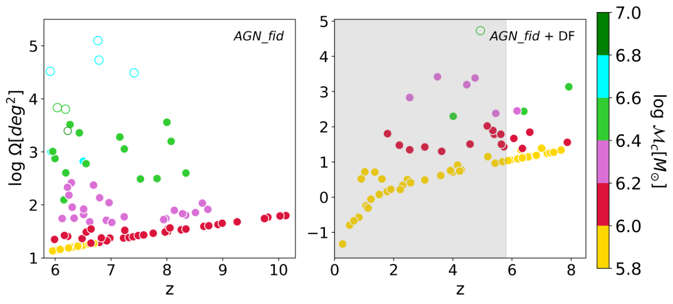
The upper left panel of fig. 7 shows the trend of the SNR with redshift, without assuming any time delay. For a given chirp mass, the further the source is located, the lower is the SNR of the GW event. Furthermore, although increases with the mass of the MBHB system, for a fixed redshift, the SNR is higher for sources with lower chirp mass. This trend occurs because low-mass binaries merge slower and enter in the LISA band sooner: hence, they stay in the LISA band for longer time and accumulate more SNR over their inspiraling lifetime. The maximum SNR that is resulting in this case is .
The upper right panel of fig. 7 shows instead the same trend of the SNR with redshift, when time delay due to dynamical friction is taken into account. We find that in this case events delayed at epochs are characterized by SNRs that can be as high as , while at the highest SNR limit remains the same as AGN_fid without any delays (SNR 150).
| Run | |||||||||
|---|---|---|---|---|---|---|---|---|---|
| AGN_fid | 145 | 0.69 | 0.9-7.0 | 0.5-30 | 0.10-0.38 | 1.9-9.3 | 0.31 | 0.04 | 0.8-4.0 |
| AGN_fid+DF | 116 | 0.66 | 0.2-3.2 | 0.0-18 | 0.10-0.9 | 0.1-9.6 | 0.31 | 0.01 | 1.33 |
| BHs_noFB | 140 | 0.46 | 0.9-6.0 | 0.7-39 | 0.09-0.38 | 1.9-9.5 | 0.50 | 0.03 | 0.7-3.9 |
| AGNcone | 583 | 0.76 | 0.6-10 | 1.1-75 | 0.09-0.42 | 1.8-10.5 | 0.22 | 0.02 | 0.4-4.7 |
| AGNsphere | 415 | 0.78 | 0.6-7.5 | 0.6-54 | 0.09-0.40 | 1.6-8.4 | 0.22 | 0.005 | 1.6-3.7 |
Finally, for the prospect of follow-up observations with electromagnetic telescopes, we calculate the LISA angular resolutions of LDEs to quantify how large is the region in the sky that must be covered by a telescope to detect the electromagnetic signals from merging MBHBs. We adopt the results found by McGee et al. 2020, which are derived from a range of population models: the median angular resolution can be associated to the median SNR at which a merger is observed by the following relation:
| (18) |
The lower panel of Fig. 7 tracks the redshift evolution of the angular resolution for LDEs. Following the SNR trend, the optimal angular resolution is found for lower redshift (higher ) and smaller chirp mass (higher SNR) systems. This figure clearly shows that, although GW events from MBHB coalescence can be detected at high-, their sky localization is poor (McWilliams et al. 2011, 10 deg2 in the most optimistic case; see also), making follow-up observations in different EM bands challenging.
5.2 Mass ratio
Fig. 8 shows how the number of LDEs is distributed in terms of the "mass ratio" (defined as , and shown in the x axis) and the "total mass" (, and shown in the y axis), for AGN_fid with (right) and without (left) considering additional delay in the mergers due to dynamical friction.
The highest fraction of LDEs occurs for equi-mass binaries, in the low mass range (), irrespective of consideration of delay time and is about 35 per cent to 40 per cent of the total LDE population in each run. In other words, "just-seeded" black holes in binaries have a higher probability to coalesce as compared to black holes with higher mass, assembled by accretion and/or merging.
Furthermore, we note that for a fixed , the larger is the mass ratio the higher is the fraction of mergers. This is simply due to the fact that the number of black holes decreases with increasing masses, thus for a fixed most of the mergers occurs for the BHs with lowest mass.

5.3 Time, frequency, and spatial scales of interest
Two MBHs1717 17 We only consider binary coalescences in our analysis, neglecting systems composed by three (or more) MBHs. at a distance require a certain time to merge through the emission of GWs. Such a time scale is called coalescing time () and defined as follows:
| (19) |
where is the initial separation of the two merging MBHs and is the symmetric mass ratio. However, as already mentioned in Sec. 5.1, we can detect the GW signal only after SNRSNRthresh. We thus compute the observational time as the time interval between the moment when SNRSNRthresh and when the two MBHs start merging:
| (20) |
which provides the period of time during which the GW event is actually observable. This timescale provides the interval of time required to eventually trigger electromagnetic telescopes for follow-up observations to find the EM counterpart of the MBHB merging (Loeb 2016, see for example), or to simply probe the host galaxies of the system.
To the observational time of a merger event we can associate the frequency and the separation of the MBHs such that SNRSNRthresh, which are related by the following expression:
| (21) |
We summarise the resulting scales of interest in Table 3.
6 Caveats and discussion
The results presented in this work are affected by several limitations:
- •
Spatial resolution: the dynamical range required to study galaxy formation and BH co-evolution through numerical simulations is extremely large, ranging from hundreds of Mpc scales (to search for massive DM halos in N-body simulations) to sub-kpc scales (required to properly model gas accretion onto BHs and the subsequent feedback processes). This implies that the spatial resolution that is possible to achieve within a reasonable amount of computational time is typical limited to tens of pc scale1818 18 The largest spatial resolution achieved so far by zoom-in cosmological simulations is 15 pc of a z = 7 quasar (Lupi et al. 2019)., namely more than 7 orders of magnitude larger than the typical scales of interest for GW studies (see Table 3).
- •
Temporal resolution: a discussion similar to the spatial resolution can be done for what concerns the temporal resolution. Black hole properties in our simulations are evolved with time-steps of Myr, which are several orders of magnitude larger than the typical scales of interest for GW studies (see Table 3). The situation gets worse if we consider the time interval between two snapshots ( tens Myr). This implies that we are not associating an LDE to the galaxy properties at the time of the coalescence (see Sec. 4.1).
- •
Seeding prescription: our simulations are based on a seeding prescription that mimicks the DCBH, given the mass of the seeds that we choose. However, the formation of a DCBH is governed by a complex network of physical processes (i.e. H2 formation, metal enrichment, radiative transfer) that is impossible to take into account self-consistently in cosmological zoom-in hydrodynamical simulations. Our seeding prescription (namely a BH of mass in each DM halo) is thus certainly overestimating the number of MBHs in 5 simulations (Vito et al. 2022, see e.g.) and consequently the expected number of merger events reported here.
For the reasons reported above, the merger rate computed in this work represents a solid upper limit on the number of merger events that LISA will be able to detect.
7 Summary and conclusions
In this work, we adopted a suite of cosmological zoom-in hydrodynamical simulations of galaxy formation and BH co-evolution, developed with the GADGET-3 code, and characterised by different numerical resolutions and star formation/AGN feedback prescriptions. Our simulations are based on a seeding prescription such that BHs are planted in DM halos; furthermore, if two BHs are at a distance smaller than the smoothing length of the simulations and their relative velocity is smaller than the local sound speed, they are assumed to merge instantaneously. We use these simulations to investigate the coalescence of massive black hole () binaries at and to compute their GW properties. We summarise below the findings of our work and draw the main conclusions arising from these results.
- •
Merger rate : We calculated the merger rates of MBHBs with different AGN feedback scenarios and numerical resolution: thermal (AGN_fid and BHs_noFB by 106, ) and kinetic (AGNcone and AGNsphere by 5, ). We found that the merger rate strongly depends on the numerical resolution adopted, ranging within 80 to 300 events per year in the 106 and 5, respectively at redshift 6. Furthermore, the merger rates of MBHBs at fixed resolution depend on the feedback recipe implemented: the AGN_fid model predicts a merger rate that is a factor 2 higher than BHs_noFB at for chirp masses in the range ; analogously, the AGNcone model predicts a merger rate that is a factor 3 higher than AGNsphere at both for low () and high () chirp masses. Different feedback prescriptions and numerical resolutions also affect the epoch of the furthest GW signal detectable with LISA: in the 106 simulations, for , the furthest GW signal occurs at while in the 5 at . We discussed in details all the physical and numerical explanations for these trends and we underlined the several motivations that make our predictions stringent upper limits to the actual merger rates that are expected to be observed.
- •
Halo bias : Our merger rate predictions are biased since they are based on zoom-in simulations targeting massive DM halos. To quantify this bias, we adopted the semi-analytical model by Barausse 2012 and showed that a MBH model like ours (with heavy BH seeds and instantaneous mergers) overpredicts the actual merger rate by a factor of 20 at comparable redshifts (z > 6). For lighter seeds as well as heavy seed models with time delays included, the merger rate overprediction still remains at a factor between 20 to 30.
- •
Delays in MBHB mergers : We corrected in post-processing the coalescing time of MBHB mergers including a time delay due to dynamical friction from the surrounding stars. We found that, if this delay is considered, 83 per cent of MBHBs will merge within the Hubble time, but only 21 per cent of them, will merge within 1 Gyr, namely the age of the Universe at .
- •
Signal-to-noise ratio and angular resolution : Taking into account the LISA frequency bands, we calculated the signal-to-noise ratio and the angular resolution of the GW events predicted by our fiducial run, AGN_fid. The fraction of LISA detectable events with high signal-to-noise ratio (SNR5) ranges between 66-69 per cent depending on the inclusion of time delays in post-processing. The largest SNR is reached in the case of low chirp masses () which, although being characterized by a smaller characteristic strain, remain in the LISA band for a longer time, thus decreasing the noise and increasing the SNR. These systems are however, characterized by very low angular resolutions (10 ).
- •
Mass ratio of LDEs : We computed the distribution of the mass ratio of the LDEs in the AGN_fid run and we found that the maximum number of mergers occurs for equi-massed binaries which are ’just-seeded’ (i.e. with ). For a fixed total mass of a MBHB, the number of mergers increases with increasing mass ratio which can be attributed to hierarchical structure formation: several low-mass MBHs merge (and accrete) to form more massive MBHs. This remained true even when further time delays in merging are considered.
One of the main goals of our study was to quantify the range of uncertainties on the merger rate of LISA detectable events. We find that considerable different merger rates result from the simulations in our suite. To get a more reliable constraint on this important issue, the shortage of currently adopted models should be addressed. For what concerns the EM signals arising from LDEs, the main challenge remains the poor LISA sky localization that in the most optimistic case ( at ) is around 10 . For this reason, it is important to further investigate the EM properties of LDEs to search for eventual, unique signatures from MBH coalescences to maximize the chances of their detections which we address in our future work.
Acknowledgements
The authors thank Andrea Pallottini, Hamsa Padmanabhan and Alessandro Lupi for their helpful insights and comments. SG acknowledges support from the ASI-INAF n. 2018-31-HH.0 grant and PRIN-MIUR 2017. MV is supported by the Alexander von Humboldt Stiftung and the Carl Friedrich von Siemens Stiftung. MV also acknowledges support from the Excellence Cluster ORIGINS, which is funded by the Deutsche Forschungsgemeinschaft (DFG, German Research Foundation) under Germany’s Excellence Strategy - EXC-2094 - 390783311. PB acknowledges support from the Brazilian funding agency FAPESP (grants 2016/01355-5, 2016/22183-8). D.I.V. acknowledges the financial support provided under the European Union’s H2020 ERC Consolidator Grant “Binary Massive Black Hole Astrophysics” (B Massive, Grant Agreement: 818691)
Data Availability Statement
The data underlying this article will be shared on reasonable request to the corresponding author.
References
- Amaro-Seoane et al. (2022) Amaro-Seoane P., et al., 2022, arXiv e-prints, p. arXiv:2203.06016
- Arun et al. (2009) Arun K. G., et al., 2009, Classical and Quantum Gravity, 26, 094027
- Arzoumanian et al. (2018) Arzoumanian Z., et al., 2018, The Astrophysical Journal, 859, 47
- Barai & de Gouveia Dal Pino (2019) Barai P., de Gouveia Dal Pino E. M., 2019, Monthly Notices of the Royal Astronomical Society, 487, 5549
- Barai et al. (2018) Barai P., Gallerani S., Pallottini A., Ferrara A., Marconi A., Cicone C., Maiolino R., Carniani S., 2018, MNRAS, 473, 4003
- Barausse (2012) Barausse E., 2012, Monthly Notices of the Royal Astronomical Society, 423, 2533
- Barausse et al. (2020) Barausse E., Dvorkin I., Tremmel M., Volonteri M., Bonetti M., 2020, The Astrophysical Journal, 904, 16
- Barkana & Loeb (2001) Barkana R., Loeb A., 2001, Phys. Rep., 349, 125
- Begelman et al. (2006) Begelman M. C., Volonteri M., Rees M. J., 2006, Monthly Notices of the Royal Astronomical Society, 370, 289–298
- Bhowmick et al. (2022) Bhowmick A. K., et al., 2022, Probing the quasars in a universe with IllustrisTNG physics: Impact of gas-based black hole seeding models, doi:10.48550/ARXIV.2205.05717, https://arxiv.org/abs/2205.05717
- Binney & Tremaine (2008) Binney J., Tremaine S., 2008, Galactic Dynamics: Second Edition
- Blanchet et al. (1995) Blanchet L., Damour T., Iyer B. R., Will C. M., Wiseman A. G., 1995, Physical Review Letters, 74, 3515
- Blecha et al. (2015) Blecha L., et al., 2015, Monthly Notices of the Royal Astronomical Society, 456, 961
- Blumenthal et al. (1984) Blumenthal G. R., Faber S., Primack J. R., Rees M. J., 1984, Nature, 311, 517
- Bondi (1952) Bondi H., 1952, MNRAS, 112, 195
- Bondi & Hoyle (1944) Bondi H., Hoyle F., 1944, MNRAS, 104, 273
- Bonetti et al. (2019) Bonetti M., Sesana A., Haardt F., Barausse E., Colpi M., 2019, Monthly Notices of the Royal Astronomical Society, 486, 4044–4060
- Booth & Schaye (2009) Booth C. M., Schaye J., 2009, Monthly Notices of the Royal Astronomical Society, 398, 53–74
- Chabrier (2003) Chabrier G., 2003, Publications of the Astronomical Society of the Pacific, 115, 763–795
- Chandrasekhar (1943) Chandrasekhar S., 1943, ApJ, 97, 255
- Ciardi & Loeb (2000) Ciardi B., Loeb A., 2000, The Astrophysical Journal, 540, 687–696
- Correa et al. (2015a) Correa C. A., Wyithe J. S. B., Schaye J., Duffy A. R., 2015a, Monthly Notices of the Royal Astronomical Society, 450, 1514
- Correa et al. (2015b) Correa C. A., Wyithe J. S. B., Schaye J., Duffy A. R., 2015b, Monthly Notices of the Royal Astronomical Society, 450, 1521
- Cutler & Flanagan (1994) Cutler C., Flanagan É . E., 1994, Physical Review D, 49, 2658
- Davies et al. (2011) Davies M. B., Miller M. C., Bellovary J. M., 2011, ApJ, 740, L42
- Dayal et al. (2019) Dayal P., Rossi E. M., Shiralilou B., Piana O., Choudhury T. R., Volonteri M., 2019, Monthly Notices of the Royal Astronomical Society, 486, 2336–2350
- DeGraf & Sijacki (2019) DeGraf C., Sijacki D., 2019, Monthly Notices of the Royal Astronomical Society, 491, 4973–4992
- DeGraf et al. (2021) DeGraf C., Sijacki D., Di Matteo T., Holley-Bockelmann K., Snyder G., Springel V., 2021, MNRAS, 503, 3629
- Devecchi et al. (2012) Devecchi B., Volonteri M., Rossi E. M., Colpi M., Portegies Zwart S., 2012, MNRAS, 421, 1465
- Di Matteo et al. (2012) Di Matteo T., Khandai N., DeGraf C., Feng Y., Croft R. A. C., Lopez J., Springel V., 2012, The Astrophysical Journal, 745, L29
- Edgar (2004) Edgar R., 2004, New Astronomy Reviews, 48, 843–859
- Eisenstein & Loeb (1995) Eisenstein D. J., Loeb A., 1995, The Astrophysical Journal, 443, 11
- Fan et al. (2006) Fan X., et al., 2006, The Astronomical Journal, 132, 117–136
- Farmer & Phinney (2003) Farmer A. J., Phinney E. S., 2003, Monthly Notices of the Royal Astronomical Society, 346, 1197–1214
- Ferrara et al. (2014) Ferrara A., Salvadori S., Yue B., Schleicher D., 2014, Monthly Notices of the Royal Astronomical Society, 443, 2410–2425
- Flanagan & Hughes (1998) Flanagan É. É., Hughes S. A., 1998, Phys. Rev. D, 57, 4535
- Haehnelt (1994) Haehnelt M. G., 1994, Monthly Notices of the Royal Astronomical Society, 269, 199–208
- Hahn & Abel (2011) Hahn O., Abel T., 2011, Monthly Notices of the Royal Astronomical Society, 415, 2101–2121
- Hartwig et al. (2018) Hartwig T., Agarwal B., Regan J. A., 2018, Monthly Notices of the Royal Astronomical Society: Letters, 479, L23–L27
- Hawking & Israel (1989) Hawking S. W., Israel W., 1989, Three Hundred Years of Gravitation. Cambridge University Press
- Heger et al. (2003) Heger A., Fryer C. L., Woosley S. E., Langer N., Hartmann D. H., 2003, The Astrophysical Journal, 591, 288–300
- Hirano et al. (2015) Hirano S., Hosokawa T., Yoshida N., Omukai K., Yorke H. W., 2015, Monthly Notices of the Royal Astronomical Society, 448, 568
- Hoyle & Lyttleton (1939) Hoyle F., Lyttleton R. A., 1939, Proceedings of the Cambridge Philosophical Society, 35, 405
- Izquierdo-Villalba et al. (2021) Izquierdo-Villalba D., Sesana A., Bonoli S., Colpi M., 2021, Monthly Notices of the Royal Astronomical Society, 509, 3488
- Jaffe & Backer (2003) Jaffe A. H., Backer D. C., 2003, The Astrophysical Journal, 583, 616–631
- Jiang et al. (2010) Jiang C. Y., Jing Y. P., Lin W. P., 2010, Astronomy and Astrophysics, 510, A60
- Johnson et al. (2012) Johnson J. L., Whalen D. J., Fryer C. L., Li H., 2012, The Astrophysical Journal, 750, 66
- Katz & Larson (2019) Katz M. L., Larson S. L., 2019, MNRAS, 483, 3108
- Katz et al. (2019) Katz M. L., Kelley L. Z., Dosopoulou F., Berry S., Blecha L., Larson S. L., 2019, Monthly Notices of the Royal Astronomical Society
- Kelley et al. (2016) Kelley L. Z., Blecha L., Hernquist L., 2016, Monthly Notices of the Royal Astronomical Society, 464, 3131
- Klein et al. (2016) Klein A., et al., 2016, Physical Review D, 93
- Knollmann & Knebe (2009) Knollmann S. R., Knebe A., 2009, The Astrophysical Journal Supplement Series, 182, 608–624
- Kormendy (2001) Kormendy J., 2001, AIP Conference Proceedings
- Koushiappas et al. (2004) Koushiappas S. M., Bullock J. S., Dekel A., 2004, Monthly Notices of the Royal Astronomical Society, 354, 292–304
- Krolik et al. (2019) Krolik J. H., Volonteri M., Dubois Y., Devriendt J., 2019, The Astrophysical Journal, 879, 110
- Latif et al. (2013) Latif M. A., Schleicher D. R. G., Schmidt W., Niemeyer J., 2013, Monthly Notices of the Royal Astronomical Society, 433, 1607
- Lentati et al. (2015) Lentati L., et al., 2015, Monthly Notices of the Royal Astronomical Society, 453, 2577
- Lodato & Natarajan (2006) Lodato G., Natarajan P., 2006, Monthly Notices of the Royal Astronomical Society, 371, 1813–1823
- Loeb (2016) Loeb A., 2016, The Astrophysical Journal, 819, L21
- Loeb & Rasio (1994) Loeb A., Rasio F. A., 1994, The Astrophysical Journal, 432, 52
- Lupi et al. (2014) Lupi A., Colpi M., Devecchi B., Galanti G., Volonteri M., 2014, Monthly Notices of the Royal Astronomical Society, 442, 3616–3626
- Lupi et al. (2019) Lupi A., Volonteri M., Decarli R., Bovino S., Silk J., Bergeron J., 2019, MNRAS, 488, 4004
- Madau et al. (1998) Madau P., Pozzetti L., Dickinson M., 1998, ApJ, 498, 106
- Magorrian et al. (1998) Magorrian J., et al., 1998, The Astronomical Journal, 115, 2285–2305
- Mapelli (2016) Mapelli M., 2016, MNRAS, 459, 3432
- McGee et al. (2020) McGee S., Sesana A., Vecchio A., 2020, Linking gravitational waves and X-ray phenomena with joint LISA and Athena observations (arXiv:1811.00050)
- McWilliams et al. (2011) McWilliams S. T., Lang R. N., Baker J. G., Thorpe J. I., 2011, Physical Review D, 84
- Mikkola & Valtonen (1992) Mikkola S., Valtonen M. J., 1992, Monthly Notices of the Royal Astronomical Society, 259, 115
- Murante et al. (2010) Murante G., Monaco P., Giovalli M., Borgani S., Diaferio A., 2010, MNRAS, 405, 1491
- Murante et al. (2015) Murante G., Monaco P., Borgani S., Tornatore L., Dolag K., Goz D., 2015, MNRAS, 447, 178
- Navarro et al. (1996) Navarro J. F., Frenk C. S., White S. D. M., 1996, The Astrophysical Journal, 462, 563
- Nelemans et al. (2001) Nelemans G., Yungelson L. R., Portegies Zwart S. F., 2001, A&A, 375, 890
- Nelson et al. (2015) Nelson D., et al., 2015, Astronomy and Computing, 13, 12
- Ostriker (1999) Ostriker E. C., 1999, The Astrophysical Journal, 513, 252
- Peebles (1980) Peebles P. J. E., 1980, The large-scale structure of the universe. Princeton University Press
- Pillepich et al. (2018) Pillepich A., et al., 2018, MNRAS, 473, 4077
- Planck Collaboration et al. (2016) Planck Collaboration Ade P. A. R., et al., 2016, Astronomy & Astrophysics, 594, A13
- Press & Schechter (1974) Press W. H., Schechter P., 1974, ApJ, 187, 425
- Quinlan (1996) Quinlan G. D., 1996, New Astronomy, 1, 35
- Reines et al. (2013) Reines A. E., Greene J. E., Geha M., 2013, The Astrophysical Journal, 775, 116
- Reinoso et al. (2018) Reinoso B., Schleicher D. R. G., Fellhauer M., Klessen R. S., Boekholt T. C. N., 2018, A&A, 614, A14
- Salcido et al. (2016) Salcido J., Bower R. G., Theuns T., McAlpine S., Schaller M., Crain R. A., Schaye J., Regan J., 2016, Monthly Notices of the Royal Astronomical Society, 463, 870
- Schaye et al. (2015) Schaye J., et al., 2015, MNRAS, 446, 521
- Sesana & Khan (2015) Sesana A., Khan F. M., 2015, Monthly Notices of the Royal Astronomical Society: Letters, 454, L66
- Sesana et al. (2004) Sesana A., Haardt F., Madau P., Volonteri M., 2004, The Astrophysical Journal, 611, 623–632
- Sesana et al. (2005) Sesana A., Haardt F., Madau P., Volonteri M., 2005, The Astrophysical Journal, 623, 23–30
- Sesana et al. (2007) Sesana A., Volonteri M., Haardt F., 2007, Monthly Notices of the Royal Astronomical Society, 377, 1711–1716
- Sesana et al. (2008) Sesana A., Vecchio A., Colacino C. N., 2008, Monthly Notices of the Royal Astronomical Society, 390, 192
- Sesana et al. (2016) Sesana A., Shankar F., Bernardi M., Sheth R. K., 2016, Monthly Notices of the Royal Astronomical Society: Letters, 463, L6
- Shang et al. (2010) Shang C., Bryan G. L., Haiman Z., 2010, MNRAS, 402, 1249
- Shannon et al. (2015) Shannon R. M., et al., 2015, Science, 349, 1522
- Sijacki et al. (2009) Sijacki D., Springel V., Haehnelt M. G., 2009, MNRAS, 400, 100
- Silk (2017) Silk J., 2017, The Astrophysical Journal, 839, L13
- Silk & Rees (1998) Silk J., Rees M. J., 1998, Astron. Astrophys., 331, L1
- Sądowski & Gaspari (2017) Sądowski A., Gaspari M., 2017, MNRAS, 468, 1398
- Smith & Caldwell (2019) Smith T. L., Caldwell R. R., 2019, Physical Review D, 100
- Springel (2005) Springel V., 2005, MNRAS, 364, 1105
- Springel & Hernquist (2003) Springel V., Hernquist L., 2003, Monthly Notices of the Royal Astronomical Society, 339, 289–311
- Springel et al. (2005) Springel V., Di Matteo T., Hernquist L., 2005, MNRAS, 361, 776
- Steinborn et al. (2015) Steinborn L. K., Dolag K., Hirschmann M., Prieto M. A., Remus R.-S., 2015, MNRAS, 448, 1504
- Tanaka & Haiman (2009) Tanaka T., Haiman Z., 2009, The Astrophysical Journal, 696, 1798
- Tornatore et al. (2007) Tornatore L., Borgani S., Dolag K., Matteucci F., 2007, Monthly Notices of the Royal Astronomical Society, 382, 1050–1072
- Valentini et al. (2017) Valentini M., Murante G., Borgani S., Monaco P., Bressan A., Beck A. M., 2017, MNRAS, 470, 3167
- Valentini et al. (2019) Valentini M., Borgani S., Bressan A., Murante G., Tornatore L., Monaco P., 2019, MNRAS, 485, 1384
- Valentini et al. (2020) Valentini M., et al., 2020, MNRAS, 491, 2779
- Valentini et al. (2021) Valentini M., Gallerani S., Ferrara A., 2021, MNRAS,
- Valiante et al. (2020) Valiante R., et al., 2020, Monthly Notices of the Royal Astronomical Society, 500, 4095–4109
- Vito et al. (2022) Vito F., Di Mascia F., Gallerani S., Zana T., Ferrara A., Carniani S., Gilli R., 2022, MNRAS, 514, 1672
- Vogelsberger et al. (2014) Vogelsberger M., et al., 2014, Nature, 509, 177
- Volonteri & Bellovary (2012) Volonteri M., Bellovary J., 2012, Reports on Progress in Physics, 75, 124901
- Volonteri et al. (2003) Volonteri M., Haardt F., Madau P., 2003, The Astrophysical Journal, 582, 559–573
- Volonteri et al. (2017) Volonteri M., Reines A. E., Atek H., Stark D. P., Trebitsch M., 2017, The Astrophysical Journal, 849, 155
- Volonteri et al. (2020) Volonteri M., et al., 2020, MNRAS, 498, 2219
- Weinberger et al. (2017) Weinberger R., et al., 2017, MNRAS, 465, 3291
- White & Rees (1978) White S. D. M., Rees M. J., 1978, MNRAS, 183, 341
- Wiersma et al. (2009) Wiersma R. P. C., Schaye J., Smith B. D., 2009, MNRAS, 393, 99
- Woods et al. (2019) Woods T. E., et al., 2019, Publications of the Astronomical Society of Australia, 36
- Wyithe & Loeb (2003) Wyithe J. S. B., Loeb A., 2003, The Astrophysical Journal, 590, 691–706
- Yoshida et al. (2008) Yoshida N., Omukai K., Hernquist L., 2008, Science, 321, 669
- Yue et al. (2013) Yue B., Ferrara A., Salvaterra R., Xu Y., Chen X., 2013, Monthly Notices of the Royal Astronomical Society, 433, 1556–1566
- Zana et al. (2022) Zana T., Gallerani S., Carniani S., Vito F., Ferrara A., Lupi A., Di Mascia F., Barai P., 2022, MNRAS,
- eLISA Consortium et al. (2013) eLISA Consortium T., et al., 2013, The Gravitational Universe (arXiv:1305.5720)
Appendix A Constraints from PTA
We compare our predictions with upper limits placed by several Pulsar Timing Array (PTA) observations. PTAs are sensitive to GWs with frequencies between to Hz. In this nano-Hz regime, the signal mostly arises from stochastic gravitational wave background (GWB) produced by the incoherent superposition of GWs from the population of inspiralling MBHBs overlapping in frequencies. The characteristic strain arising from this stochastic GWB can be written as (Sesana et al. 2008):
| (22) |
where is the comoving number density of MBHB merger per unit redshift, and rest-frame chirp mass, is the frequency of the GWs in the observer frame, and is the energy emitted per logarithmic rest-frame frequency, .
Assuming the inspiralling population of MBHBs in the PTA band are in perfect circular orbits, Eq. 22 can be re-written as:
| (23) |
This type of relation is typically written as:
| (24) |
where is the amplitude of the signal at the reference frequency which is usually normalized at , and is typically denoted as .

We present our predictions in Fig. 9, where we apply a bias correction factor of 20 (see Sec. 3.2). We find , which is below the upper limits placed by the NANOGrav (Arzoumanian et al. 2018), EPTA (Lentati et al. 2015) observations and the PPTA observations (Shannon et al. 2015). We emphasize that our predictions do not include any contribution from sources at , which are instead expected to dominate the background (Izquierdo-Villalba et al. 2021, e.g.).
Appendix B Time delay due to stellar hardening
Stellar hardening is the process by which stars interact with the MBHB and gradually become more tightly bound to it over time. For already bound MBHBs, the gravitational field can be strong enough to disrupt the orbits of nearby stars. As a result, some of these stars can be captured by the MBHB and start to orbit around it (Mikkola & Valtonen 1992). As these stars continue to interact with the binary, they can extract energy and angular momentum from the MBHB, causing it to become more tightly bound (Quinlan 1996).
We compute the stellar hardening timescale following Sesana & Khan 2015:
| (25) |
where and are the velocity dispersion and the stellar density at the sphere of influence1919 19 The sphere of influence is approximated as the sphere containing twice the binary mass in stars., and is the transition separation of stellar hardening and GW hardening at which the binary spends most of its time:
| (26) |
| (27) |
| (28) |
where is the radius containing twice the binary mass in stars:
| (29) |
and we assume the index = 2 (Volonteri et al. 2020) and Sesana & Khan 2015.
Finally, the total time of the MBHB merger including dynamical friction and stellar hardening is given by:
| (30) |
According to the formalism reported above, we find that varies in the range 1-10 Gyr, since central stellar densities are in the range 40-600 . These values are not a fair representation, likely because the resolution of our simulations do not allow us to properly determine the matter distribution on such small scales. For comparison, in Sgr A∗ . In addition, galaxies at high redshift are likely more centrally concentrated than local galaxies. Thus, we would expect values even larger than what is found in Sgr A∗. For all these reasons, we do not include the delay due to stellar hardening in our post-processing calculations.
Appendix C GW detectables for different simulation runs
Here we show the comparison of different GW detectables for the simulation runs AGNcone, AGNsphere and BHs_noFB compared with AGN_fid. In all cases we report the results for a biased halo with no delays in post-processing.


Fig. 10 shows the redshift distribution of SNR (upper panel) and angular resolution (lower panel) of the GW events for different chirp masses in our four different simulation suits. The overall trend in the SNR and resolution distribution is explained in Sec. 5.1. Since only in the 5 simulations the chirp mass PDF is populated for , this explains why for these simulations the SNR predicted reaches the highest value (SNR160). Apart from this aspect (and the different number of events predicted, already discussed in Sec. 3.1), we do not find in the SNR predictions huge differences among different models. Consequently, the corresponding angular resolutions of event the loudest GW events remain quite poor () for all models.
In Fig. 11, we also show the fraction of mergers are distributed in the "mass ratio" and "total mass" plane, in the four simulation runs analysed in this work. The different coverage of the "mass ratio"-"total mass" plane simply reflects the different numbers of LDEs in the simulations runs: as shown in table 3 a higher number of LDEs occurs in the AGNcone run, which shows the most densely populated "mass ratio"-"total mass" plane, while the smaller number of LDEs is predicted in the BHs_noFB run.
As seen in Sec.5.2, highest fraction of LDEs occurs for equi-mass binaries, in the low mass range (), independent of the feedback implemented and the simulation resolution and it ranges between 20 per cent and 40 per cent of the total LDE population in each run.
