Evolution of Cosmological Parameters and Fundamental Constants in a Flat Quintessence Cosmology: A Dynamical Alternative to CDM
Rodger I. Thompson
Department of Astronomy and Steward Observatory University of Arizona; rit@arizona.edu
1 Abstract
The primary purpose of this work is the provision of accurate, analytic, evolutionary templates for cosmological parameters and fundamental constants in a dynamical cosmology. A flat quintessence cosmology with a dark energy potential that has the mathematical form of the Higgs potential is the specific cosmology and potential addressed in this work. These templates, based on the physics of the cosmology and potential are intended to replace the parameterizations currently used to determine the likelihoods of dynamical cosmologies. Acknowledging that, unlike CDM, the evolutions are dependent on both the specific cosmology and the dark energy potential the templates are referred to as Specific Cosmology and Potential, SCP, templates. The requirements set for the SCP templates are that they must be accurate, analytic functions of an observable such as the scale factor or redshift. This is achieved through the utilization of a modified beta function formalism that is based on a physically motivated dark energy potential to calculate the beta function. The methodology developed here is designed to be adaptable to other cosmologies and dark energy potentials. The SCP templates are essential tools in determining the relative likelihoods of a range of dynamical cosmologies and potentials. An ultimate purpose is the determination whether dark energy is dynamical or static in a quantitative manner. It is suggested that the SCP templates calculated in this work can serve as fiducial dynamical templates in the same manner as CDM serves for static dark energy.
Keywords:
Cosmological Parameters ; Fundamental Constants; Quintessence
2 Introduction
This manuscript examines the evolutions in the late time, matter and dark energy dominated, epoch between the scale factors of 0.1 and 1.0 for a flat quintessence cosmology. This epoch is the primary focus of the upcoming Rubin and Roman observatories observations. The study does not consider radiation but only matter and dark energy and is therefore only relevant to late epochs not under the influence of radiation. The farthest look back time considered here is at a scale factor of 0.1 where radiation has no measurable effect.
Some preliminary aspects of areas covered in this publication are discussed in 2022. This work, however, expands the study and is intended for both experts in the field and those who wish an introduction to calculations of the evolution of cosmological parameters and fundamental constants. The methodology presented here is particular to the specific cosmology, quintessence, and the evolutionary templates it calculates are for a specific dark energy potential. The templates from the methodology are therefore referred to as Specific Cosmology and Potential, SCP, templates.
The nature of dark energy has been declared one of the “grand challenges in both physics and astronomy” by the Decadal Survey of Astronomy and Astrophysics 2022 (National Academies of Sciences, Engineering, and Medicine 2021). A major part of that challenge is the question of whether dark energy is static or dynamic. An important aspect of the question is whether a dynamical cosmology can fit the current and future observational data as well or better than CDM. This work explores a flat quintessence cosmology with current parameter boundary conditions close but not equal to CDM to provide accurate predictions of parameter and fundamental constant evolutions for comparison with data. The calculation of the evolutions is described in detail, particularly the use of a modified beta function formalism that produces accurate, analytic, functions of the parameters and constants as a function of the observable scale factor. The dark energy potential has a natural origin, having the same mathematical polynomial form as the Higgs potential. It is, however, not the Higgs field and has none of the rich physics of the Higgs. It is simply a rolling scalar field with quintessence physics that is coupled to gravity. Since the potential has the same mathematical form as the Higgs potential it is referred to as the Higgs Inspired or HI potential.
The development of the SCP templates for a flat, minimally coupled, Quintessence cosmology takes advantage of the property of minimally coupled systems that the dark energy and matter density evolutions are independent of each other. Each can be calculated separately, as is traditionally done for Quintessence. (Scherrer and Sen 2008; Copeland 2006; Cicciarella and Pieroni 2017; 2018), and then combined when necessary for the calculation of the cosmological parameters such as the Hubble parameter. As an example the evolution of the matter density is simply where is the current matter density and is the scale factor. The evolution of the scalar and other dark energy functions are calculated in sections 4 through 11 without reference to the matter density except in the introduction of the Friedmann constraints. The matter density is incorporated in section 12 where the Hubble parameter is calculated using the first Friedmann constraint. An approximation is made in equation 16 where the term is set to zero to achieve equation 17 which is only a function of the dark energy potential and scalar. The approximation is valid for all of the dark energy EoS values in this study but could lose accuracy for high deviations of from minus one.
Beyond demonstrating the methodology for producing SCP templates for cosmological parameter evolution this work also examines the role of fundamental constants in setting constraints on both static and dynamical cosmologies. Without invoking special symmetries it is difficult to prevent a scalar field that couples with gravity from also coupling with other sectors such as the weak, electromagnetic and strong forces (Carroll 1998). The values of the fundamental constants such as the fine structure constant and the proton to electron mass ratio are determined by the Quantum Chromodynamic Scale , the Higgs vacuum expectation value and the Yukawa couplings (Coc 2007). It is assumed here that the HI scalar responsible for dark energy also interacts with these sectors. The temporal evolution of the constants produced by the interactions is examined in section 18 along with the connection to the dark energy Equation of State, EoS, .
The study utilizes natural units with , and set to one where is the Newton gravitational constant. The mass units are reduced Planck masses . The constant is the inverse reduced Planck mass . In the mass units of this study but it is retained in equations to display the proper mass units.
3 The Need for SCP Templates
The SCP templates generated in this study are candidates for a fiducial set of templates to compare with the observations in the same way that the well known static CDM templates are currently used. Although accurate analytic templates for the static CDM cosmology exist similar templates for dynamical cosmologies are exceedingly rare. Currently the primary tools for analyzing dynamical cosmologies are parameterizations such as the Chevallier, Polarski and Linder , CPL, (Chevallirer 2001; Linder. 2003) linear parameterization of the dark energy Equation of State, EoS, . Such parameterizations do not contain any of the physics of the dynamical cosmology and its dark energy potential. Figure 1 shows the CPL fit to a quintessence cosmology with the dark energy potential described in section 6.

The linear CPL, dashed line, is a poor fit to the true evolution, solid line, and is not an accurate measure of its likelihood. Beyond producing an erroneous likelihood the CPL fit also produces erroneous conclusions. At scale factors greater than 0.8 the CPL fit is in the phantom region, , even though the true evolution has no phantom values. It is well known that it is quite difficult for quintessence to cross the phantom boundary (Vikman 2005). Three recent analyses of observational data (Planck Collaboration 2019; Di Valentino, Melchiorri and Silk 2020; Di Valentino 2020) using a MCMC analysis with a CPL dark energy template find phantom values of at low redshift. The presence of phantom values of can be interpreted as strong evidence against quintessence, however, figure 1 clearly shows that for a quintessence cosmology, with no phantom values, a CPL fit erroneously produces phantom values due to fitting a non-linear evolution with a linear parameterization. The methodology described here produces templates based on the action of the quintessence cosmology and a specific dark energy potential for comparison to the observational data. SCP templates are essential to properly compare accurate predictions to the observational data in establishing the true likelihood of the cosmology and potential.
4 Quintessence
As one of the simplest dynamical cosmologies, flat quintessence provides a straightforward example of a methodology for producing SCP templates. Quintessence is a well studied (Copeland 2006) and well known cosmology but for easy reference some important aspects of its physics are given here.
The quintessence cosmology is defined by its action .
| (1) |
where is the dark energy action and is the matter (dust) action. is the Ricci scalar, is the determinant of the metric , is the scalar, and is the dark energy potential. The scalar is the true scalar with a value on the order of . A second scalar is introduced in section 6 for the Ratra-Peebles form of the dark energy potential. This scalar is, therefore, referred to as the Ratra-Peebles, or RP scalar and has a value on the order of unity in units of . In the matter action is the current matter density and is the scale factor. The matter component of the total action is separate from the quintessence dark energy component resulting in a total action of as in equation (3.1) of (Cicciarella and Pieroni 2017) The matter component is introduced via the first Friedmann constraint in section 12 in the calculation of the Hubble parameter. In the following only dark energy is considered in the derivation of the scalar since its evolution is not affected by matter. Matter is then introduced in section 12 to derive the proper Hubble parameter that includes both dark energy and matter.
The kinetic component of is
| (2) |
The common kinetic symbol for is used throughout the manuscript. is a function of only time since the universe is assumed to be spatially homogeneous.
The quintessence dark energy density and pressure are set by the action as
| (3) |
In natural units both the density and the pressure have units of and the time derivative of the scalar has units of . The dark energy EoS is
| (4) |
which is a pure number. Combining eqns. 3 gives
| (5) |
It follows that
| (6) |
giving a relationship to the dark energy EoS and the dark energy density.
| (7) |
5 General Cosmological Constraints
Independent of the particular cosmology there are general constraints on the evolution of the cosmological parameters. The first are the Friedmann constraints.
5.1 The Friedmann constraints
The two Friedmann constraints play an important role in calculating the SCP templates. The forms of the first and second Friedman constraints used here are
| (8) |
where is the dark energy density, is the matter density, is the sum of the matter and dark energy densities and is the dark energy pressure. In a universe with only dark energy the Friedmann constraints are
| (9) |
where denotes the dark energy only Hubble parameter. The critical density is and the ratios of the dark energy density and matter density to the critical density are and that add to one in a flat universe. The dark energy only Hubble parameter is then .
5.2 The Boundary Conditions
Since we are looking for solutions of differential equations the second set of constraints is imposed by the boundary conditions, the current values of certain cosmological parameters. Table 1 displays the cosmological boundary conditions chosen for this study. The range of the scale factor is slightly arbitrary but is set to include the range covered by the Rubin and Roman observations. The range of is set close to minus one to be near but not exactly minus one. The value is set to 73 consistent with the current late time expectations (Riess et al. 2022). and are the current concordance values. All of the boundary conditions appear in the evolutionary functions of the SCP templates and are therefore easily changed.
| scale factor | ||||||
|---|---|---|---|---|---|---|
| 73 | 0.3 | 0.7 | -0.99 | -0.995 | -0.999 | 0.1 - 1.0 |
6 The Higgs Inspired Potential
The dark energy potential has the mathematical form of the Higgs potential a quartic polynomial with a constant . It is chosen for two reasons. The first is that the mathematical form is identical to the Higgs potential which gives rise to a scalar field that is known to exist and is therefore physically motivated, hence the name Higgs Inspired or HI potential. A second reason is that by varying the constant term it produces dark energy equations of state that are freezing, thawing, and transitioning between freezing and thawing. This makes it a good choice for a fiducial potential that covers a wide range of evolutions.
The most convenient form for the potential is a modified Ratra Peebles format (Ratra and Peebles 1988; Peebles and Ratra 1988) with a scalar field denoted by , the RP scalar introduced in section 4 that has units of mass in . The potential is then
| (10) |
where the true scalar is . and are constants with units of mass and both and are dimensionless therefore all of the dimensionality is in the leading term. Since both arguments are dimensionless there is no need for the in the usual Ratra Peebles format. The terms and replace the scalar and terms to differentiate them from the true scalar and constant which have values on the order of . The values of and are of the order unity, The value of is chosen to be greater than the current scalar to place the equilibrium point in the future. This makes the constant the dominant term followed by the two dynamical terms and in descending order.
7 The Quintessence Methodology
The methodology developed here is for the specific quintessence cosmology and only applies to a cosmology whose action is given by equation 1. Among the current plethora of dynamical cosmologies there are some with quite different names that have the same action as quintessence where this methodology will apply but not for cosmologies such as k-essence that has a different action. The methodology is demonstrated with the modified Ratra Peebles HI potential of equation 10.
7.1 The Modified Beta Function Formalism
The key to producing SCP templates that are accurate analytic functions of the scale factor is the beta function formalism (Binetruy et al. 2015; Binetruy, Mabillard & Pieroni 2017; Cicciarella and Pieroni 2017; Kohri and Matsui 2017). The beta function is a differential equation relating the scalar to the scale factor allowing the calculation of an analytic form of . The analytic form for the scalar is achieved via the approximation of a dominant potential component of the dark energy density that allows the exclusion of the kinetic component to calculate the beta function given in equation 17. This, in turn, enables the calculation of the analytic function for the scalar. The cosmological parameters are analytic functions of the scalar that are quite accurate but not exact. The cosmological parameter templates do not contain any numerical calculations.
The primary beta function formalism papers relative to this work are (Binetruy et al. 2015; Cicciarella and Pieroni 2017). The work by (Binetruy et al. 2015) considers a quintessence dark energy only universe while the work of (Cicciarella and Pieroni 2017) considers a quintessence universe with both matter and dark energy which is the universe considered in this work. Both (Binetruy et al. 2015) and (Cicciarella and Pieroni 2017) consider the general physics of the beta function formalism rather than the explicit evolution of cosmological parameters. Their approach is therefore modified in this work to provide analytic evolutionary templates for cosmological parameters. These modifications are noted in the following discussion.
The generalized beta function (Binetruy, Mabillard & Pieroni 2017) is defined as
| (11) |
From equation. 3 for the quintessence dark energy pressure it is evident that is one, giving a quintessence beta function of
| (12) |
From equation 12 and the definition of the quintessence beta function and the Hubble parameter
| (13) |
The dark energy only Hubble parameter is used in equation 13 to be consistent with the dark energy only derivation of the scalar, however, when the matter density is introduced in section 12 the Hubble parameter for both dark energy and matter should be used since it sets the time evolution of the scale factor . Equations 7 and 13 provide the useful relation
| (14) |
Since the beta function formalism is developed for dark energy the first Friedmann constraint in equation 9 applies and
| (15) |
where now the subscript designates the dark energy density.
In (Binetruy et al. 2015; Cicciarella and Pieroni 2017) the beta function is defined as the negative of the logarithmic derivative of the dark energy density. To achieve the desired analytic SCP templates equation 15 is rearranged to a slightly modified density
| (16) |
noting that for all of the cases considered here . Using the modified density the beta function is then the negative of the logarithmic derivative of the analytic HI potential.
| (17) |
The leading constant, , in the dark energy potential does not appear in the logarithmic derivative defining the beta function leaving it as an adjustable parameter to satisfy the Friedmann constraints. Note that the approximation that is equivalent to the statement that the kinetic term is small compared to the dark energy potential. This is roughly equivalent to the slow roll condition often used in evaluating dynamical cosmologies. In fact equation 17 is the negative of the first slow roll condition. The first slow roll condition is often set to a small constant, eg. (Scherrer and Sen 2008), which is only valid for an exponential potential. Here the approximation of a small value of is only used to calculate the analytic form of the scalar and the non-constant time derivative of the scalar is used in all parameter calculations. The approximation that is set to zero in determining the beta function also means that the Hubble parameter is not used in the derivation of the scalar and that its value of either or is not a factor.
Although the beta density is slightly different than the real density, application of the boundary conditions and the Friedmann constraints produces evolutionary SCP templates of high accuracy as illustrated in section 16.
7.1.1 The beta function for the HI potential
Using the HI potential in equation 10 the negative of the logarithmic derivative is
| (18) |
where the last term is from equation 14. Solving the equation formed by the last two terms for the current time yields the current value for the scalar which is an important boundary condition.
| (19) |
Since the argument of the square root in the numerator is greater than 16 equation 19 is the positive solution of the quadratic equation.
7.2 The scalar as a function of the scale factor
An essential step in achieving SCP templates as analytic functions of the scale factor is finding the scalar as a function of . From the definition of the beta function in equation 17 the differential equation for the scalar as a function of the scale factor is
| (20) |
Separating the scale factor and scalar terms gives
| (21) |
An integral of both sides of equation 21 from 1 to for the left side and from to on the right side gives
| (22) |
Equation 19 provides the value of . The following manipulations from (2022) provide a solution for involving the Lambert W function in terms of a constant and the scale factor. Dividing both sides of equation 22 by gives
| (23) |
Taking the exponential of both sides of equation 23 and dividing again by yields
| (24) |
Equation 24 has the mathematical form of the Lambert W function that is the solution to
| (25) |
where
| (26) |
Equations 25 and 26 provide an analytic solution for
| (27) |
that is the positive solution for the square root which is real since is negative. The following variable changes produce a concise form for .
| (28) |
which yields
| (29) |
Equation 29 provides the key to transforming evolutions that are a function of the scalar into functions of the observable scale factor to produce the SCP templates.
The term appears often in this manuscript. In terms of the Lambert W function it is
| (30) |
The form of the HI potential is then
| (31) |
The beta function also has a compact form in the W function format
| (32) |
7.3 Summary of the methodology
Although the methodology may appear to be complex the separate steps of the quintessence beta function formalism are relatively simple. The quintessence beta function is given in equation 12 which connects the scalar to the scale factor . As stated in the text the beta function is defined as the negative of the logarithmic derivative of the dark energy density but here it is noted that the kinetic term in the density is small compared to the potential term and a legitimate approximation is to ignore it and set the beta function to the negative of the logarithmic derivative of the potential as given in equation 17. This is the only place in the methodology that is set to zero. The kinetic term , as shown in equation 15, is used in all subsequent calculations of the templates. Equation 18 shows the beta function calculated from equation 17 and is shown in differential form in equations 20 and 21. The solution for is achieved through mathematical manipulation to the simple form in equation 29. This provides a solution for a cosmological parameter as a function of the scale factor if the solution as a function of the scalar is known.
Since the matter (dust) action is separate from the dark energy action the evolution dark energy scalar is calculated from the dark energy action as described above. The matter is included in section 12 that derives the Hubble parameter which is a function of the dark energy and matter. It is added to the total density in equation 38 for the first Friedmann constraint and is present in the Hubble parameter template in equation 40. This is the Hubble parameter that is used in the calculation of the time derivative of the scalar . Adherence to the Friedmann constraints and the inclusion of the matter density in the Hubble parameter that calculates produces accurate SCP templates that are functions of both the matter and the dark energy densities and conforms to both Friedmann constraints.
8 The Cosmology of
Before moving on to consider the evolution of , and other parameters it is worthwhile to examine the cosmology embedded in the evolution of . A thorough discussion of the mathematical properties of the Lambert W function is in (Olver, F. W. F., Lozier, D. W., Boisvert, R.F., and Clark, C.W 2010). There it is shown that has negative values if its argument is between and zero which is true for all cases considered here. This makes the argument of the square root in equation. 29 positive producing a real value of the scalar . Figure 2 shows the evolution of the principal branch of . The formal designation of the principal branch is but the subscript is dropped in the following since only the principal branch is used in this work.

Figure 2 shows the evolution of ) as a solid line for negative and a dashed line for positive . The negative portion of the Lambert W function terminates at while the positive portion continues indefinitely. Only the negative portion has real solutions for the scalar. Equation 26 shows that is negative for all positive values of the scale factor . Evolution in figure 2 proceeds from right to left as the top arrow indicates. The variable is zero when therefore the big bang is at shown by the vertical thin line. The dashed vertical line just to the left of the big bang shows the maximum excursion of the greatest evolution case, and . All of the cases considered here have values much less than one which means that .
Figure 3 shows the detail of the evolution region of figure 2. The black solid and dashed lines are the same as in figure 2 but only for the evolution region between the thick dashed and thin solid vertical lines. The first case, in red, with the highest and largest deviation of from minus one has the most extensive evolution with the right end of the evolution, , significantly after the big bang. Note that the evolutions which actually overlap the black lines have been shifted downward for visibility. The third case with the lowest value of and the least deviation of from minus one has the least evolution with its start at and its maximum of barely visible on the diagram. The middle excursion with = 2 and = -0.995 starts with = and a current of . The similar numbers are due to the end scale factor being ten times the beginning scale factor. Recall that is not time so that a small value of does not mean that the scale factor of 0.1 is very near the big bang. As hinted at in figure 2 the evolution region’s small extent make the evolutionary tracks in to appear linear. Figure 3 is an indication, verified later on, that the value of has a strong influence on the SCP templates. The upper left of the figure shows the color code of the values and the line styles of the values maintained through out the manuscript.

The black sloped solid and dashed line is the same as in Figure 2 for the small expanded region. The red solid and green dashed line are the evolutions of the , and the cases. The long dashed blue evolution for the is so short that it appears only as a small dot near below the and 2 evolutions. The evolutions are offset downward from the black track for visibility.
To aid comprehension of Figure 3 table 2 gives the value of at scale factors of 01., 0.5 and 1.0 for all values of and . All values of are negative The magnitude of increases with increasing values of and higher deviations of from minus one. The time evolution of the tracks in Figure 3 is from right to left, the same as in Figure 2. The time extents for all tracks are the same, to 1.0, but the evolution of has a large variation.
| The Values of | |||||
| scale factor | |||||
| . | 0.1 | 0.5 | 1.0 | ||
| 1. | -0.99 | 2.024 | |||
| 1. | -0.995 | 2.206 | |||
| 1. | -0.999 | 2.698 | |||
| 2. | -0.99 | 8.437 | |||
| 2. | -0.995 | 11.885 | |||
| 2. | -0.999 | 26.492 | |||
| 3. | -0.99 | 49.776 | |||
| 3. | -0.995 | 106.479 | |||
| 3. | -0.999 | 640.859 | |||
8.1 Past Evolution
The main content of this manuscript is the past evolution from the present to a past scale factor of 0.1 which is a redshift of nine. This encompasses a large fraction of the history of the universe in the matter and dark energy dominant epochs. An important question is how far back can the SCP templates be utilized. A hard limit is the onset of the radiation dominated epoch since the radiation density is not included in the present work. A reasonable limit is when the radiation density is of the matter density. The present matter density for and of 0.3 is and a present radiation density of . The radiation density is of the matter density at a scale factor of 0.0168 or a redshift of 58.5. This is strictly a physics limit on the validity of the templates. Figures 2 and 3 plus table 2 indicate that the template for the scalar is valid back to this limit but the templates have not been tested for mathematical stability at scale factors smaller than 0.1. Inclusion of the radiation density is beyond the scope of this work but it can probably be included in the same manner as the matter density.
8.2 Future Evolution
A perhaps even more intriguing question is how far in the future can the templates be extended. The solution of is analytic at scale factors greater than one which is all of the region to the left of the dashed vertical line in Figure 2. There is a limit however to the principal branch of the Lambert W function at . Figure 2 marks this location with a O at . Equation 29 shows that at which is an equilibrium point where the dark energy potential is zero. The scale factor, , where this occurs is given by
| (33) |
where and are the same as in equation 28. The values of are listed in the last column of Table 2. It is beyond the scope of this manuscript to determine whether this is a stable equilibrium point. If it is a stable equilibrium, with also zero, then it would be the end of dark energy acceleration. The universe would return to a matter dominated evolution. with making a graceful exit from acceleration. The speed of expansion would be
| (34) |
The universe would then evolve in a classical manner, slowing down to zero expansion at infinity. Given the past history of the universe it is reasonable that the lowering level of total density might reveal a new source of accelerated expansion whose density is below that of the current density.
9 The Evolution of the Scalar and the Beta Function
The scalar and the beta function influence the evolution of all of the cosmological parameters in this study. The sections below document their evolution.
9.1 The Evolution of
Figure 4 shows the evolution of the scalar over the scale factors considered in this work. The colors and line styles are consistent with the previous figure.

The values for the case are labeled on the plot. The order and line styles are the same for the other two values. The evolution is relatively small consistent with a slow roll. As expected the scalar values are monotonically increasing. The most striking feature is that the second derivative of the evolution changes from positive for to almost zero for to negative for . The three, seemingly arbitrary, delta values were chosen to illustrate this transition. The transition has a large effect on some parameters, such as the dark energy EoS, , but relatively little effect on the Hubble parameter as is shown later in Figure 7.
9.2 The Evolution of
The beta function evolution is shown in figure 5
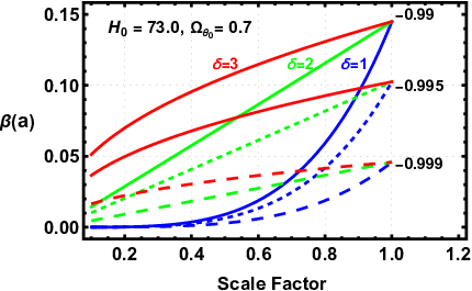
Although the general nature of the evolution of the beta function is different from the scalar it shows the same change in the second derivative of the evolution, positive for , almost zero for and negative for . The absolute value of is small and decreases as approaches minus one. The current value of beta, is identical for a given value of due to equation 14 which sets at where the subscript 0 indicates the current values. The beta function appears in many cosmological parameters due to equation 13 that links and the Hubble parameter.
10 The Value of in the Dark Energy Potential
At this point the value of in equation 10 has not been calculated. The Friedmann constraints and equation. 3 provide the means of calculating . The dark energy density is
| (35) |
Using
| (36) |
Since is a constant it can be set using the current boundary conditions which insures adherence to the first Friedmann constraint at a scale factor of one. This eliminates any constant offsets due to the approximation in equation 17 further improving the accuracy of the templates.
Rearranging equation 36 and using the current values of the parameters gives
| (37) |
11 The Evolution of the HI Dark Energy Potential
The evolution of the dark energy potential can now be calculated. Figure 6 shows the evolution of the HI dark energy potential for all of the cases.
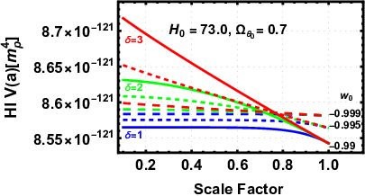
Figure 6 shows that there is only a small evolution of the potential between scale factors of 0.1 and 1.0, again consistent with a slow roll. The maximum evolution is for the case. The evolutions are essentially constant, mimicking CDM, until a scale factor of and then decrease slightly to the value for and -0.995. The cases deviate from constant evolution earlier than the cases, The cases have almost linear evolution and have the highest values, particularly at small scale factors. All of the cases have a very flat evolution. For a given value of the current value of the potential is the same for all values. From eqns. 10 and 37 the potential at a scale factor of one is . Equation 14 shows that the value of the beta function at a scale factor of one is making the same for a given .
12 The Hubble Parameter
The calculation of the Hubble parameter for the real universe requires the inclusion of both dark energy and matter. In (Cicciarella and Pieroni 2017) matter is introduced via a differential equation involving the Hubble parameter and the beta function. Here the Friedmann constraints are the primary tools for deriving the Hubble parameter in a universe with both matter and dark energy. The first Friedmann constraint gives
| (38) |
Here is the current matter density and is the mass density as a function of the scale factor. Using equation 13 is substituted for in equation 38 to obtain
| (39) |
The Hubble Parameter is therefore
| (40) |
12.1 The Time Derivative of the Hubble Parameter
The second Friedmann constraint in eqns. 9 provides the method for calculating .
| (41) |
where in units of the reduced Planck mass.
12.2 The Evolution of the Hubble Parameter
Figure 7 shows the evolution of the Hubble parameter for all values of and plus CDM. At the resolution of the figure all of the tracks overlap each other to the thickness of the line.

The dashed line on figure 7 shows the time derivative of the scale factor to show the transition to acceleration of the expansion of the universe. It occurs at a scale factor of consistent with current observations eg. (Dahiya 2022). The track has been multiplied by ten to remove its overlap with the H parameter track. The following section shows the percentage deviation of the HI Hubble parameters from CDM for all of the cases
12.3 The Percentage Deviation from CDM
The fractional deviation of the HI Hubble parameters from CDM is given by
| (42) |
Figure 8 shows the percentage deviation of the HI H parameters from the CDM H parameter.

The figure readily shows that the percentage deviation of the HI Hubble parameter from CDM is exceedingly small. The highest deviation is for the , and the smallest deviation is for the , case. All of the cases have a negative deviation indicating that the HI Hubble parameter is slightly less than CDM while the other values have positive deviations with the HI Hubble parameter slightly higher than CDM. The maximum deviations occur at scale factors between 0.6 for and 0.8 for where dark energy begins to dominate. The overall shape of the deviations are reasonable. The deviation is zero at since it set by the boundary condition. After the peak the deviation drops again as the density becomes matter dominated. Currently the deviations of the cases are impossible to detect observationally and the highest deviation is below the detection limit of the proposed near future facilities. Further discussion of the implications of the HI quintessence cosmology appears in section 17.
13 The Scale Factor and Time Derivatives of the Scalar
The scale factor and time derivatives of the scalar are not observables but are essential for the calculation of the SCP templates. The starting point is the derivative of the Lambert W function in equation 43
| (43) |
From this base the derivative of the scalar with respect to the scale factor is
| (44) |
The derivative of the scalar with respect to time is then
| (45) |
Figure 9 shows the evolution of in units of for all of the cases along with a more detailed plot of the region between a scale factor of 0.4 and 1.0.

The units of are since has the units of mass and time has units of inverse mass. In figure 9 is multiplied by to show the value of the time derivative of the true scalar . In the left panel the full evolution of is shown for the scale factors between 0.1 and 1.0 Unlike the scalar the magnitude of is decreasing for but increasing for with corresponding differences in the second derivative. The right hand panel shows the evolution between scale factors of 0.4 and 1.0 in more detail. Close inspection of the and track show that it was initially decreasing but is currently increasing. This non-monotonic evolution is also present in the dark energy EoS described later.
14 The Dark Energy Density and Pressure
Several cosmological parameters depend on the evolution of the dark energy density and pressure. Equation 3 gives the functions for them in terms of the kinetic term and the dark energy potential. Figure 10 shows the evolution of the dark energy density for all of the cases.

As usual the evolutions have a different character from the other two. The density evolution for is essentially flat and the highest evolution case, , only changes by . For all values of the density has a slight rise near a scale factor of one. For scale factors less than 0.6 the densities are essentially constant acting like a cosmological constant in the matter dominated epoch. For and 3 the density is monotonically decreasing with increasing scale factor. The second derivative of the decrease of density for the case changes from negative to positive with increasing scale factor similar to the scalar. The decrease in density for the case is larger than for the other two cases but is still only on the order of for the maximum case. Unlike the case the second derivative of the evolution is negative at all scale factors.
Figure 11 shows the evolution of the dark energy pressure.

The dark energy pressures have their characteristic negative values and, although more than the density, the absolute evolution is relatively small. The and 3 evolutions are monotonically positive and negative respectively but the pressure evolutions have stronger transitions from negative to positive than the density. As in the dark energy density the evolution is quite flat as would be expected for a value so close to minus one.
15 The Dark Energy Equation of State
By definition the dark energy EoS is the ratio of the dark energy pressure to the dark energy density. Figure 12 shows the evolution of .

The evolution is the classic thawing evolution where is initially near minus one and then thaws to the less negative values of . The is the classic freezing case where starts at values less negative than minus one and then freezes toward minus one. The evolution, however, is non-monotonic, starting as a freezing solution, and then transitioning to a thawing evolution. These evolutions mirror the evolution of the dark energy pressure in figure 11 since the magnitude of the pressure evolution is greater than the evolution of the density. The author does not know of any similar case in the literature but suggests that it may be called the freeze and thaw evolution. Figure 12 demonstrates the motivation for the simple choices of one, two and three for the values. The cases have late time evolutions very similar to CDM but significant and observable deviations at early times. The evolutions of are indistinguishable from CDM at early times and only slightly deviant from CDM at late times due to the purposely chosen values very near minus one. The evolution of would not be distinguishable from CDM with current analysis techniques. These aspects are discussed more thoroughly in section 17 that considers the HI quintessence as a candidate for a fiducial dynamical cosmology in the same way that CDM is a fiducial static cosmology.
16 The Accuracy of the Cosmology and Dark Energy Potential
At this point the SCP evolutionary templates of all of the cosmological parameters considered in this work are calculated. It is appropriate then to consider the accuracy of the cosmology and HI potential as a whole. The metric for the accuracy utilized here is the accuracy of the two Friedmann constraints which contain the Hubble parameter and its time derivative, the dark energy density and pressure plus the matter density and HI potential. Other parameters such as the dark energy equation of state are functions of the parameters in the Friedmann constraints. The first and second Friedmann constraints are given in equation 8. The two constraints are considered separately below.
16.1 The Accuracy of the First Friedmann Constraint
The left and right sides of the first Friedmann constraint should be equal therefore the accuracy, , is determined by
| (46) |
The results for all of the cases are similar in the overall magnitude but of course dissimilar in detail. The results for and the three values of are shown in figure 13.

It is obvious that the first Friedmann constraint is satisfied to better than one part in . This is on the order of the digital accuracy of the Mathematica code used in the calculation.
16.2 The Accuracy of the Second Friedmann Constraint
The second Friedmann constraint explicitly covers more parameters including the time derivative of the Hubble parameter. The fractional error for the second Friedmann constraint is given by
| (47) |
Unlike the first Friedmann constraint where all of the terms are positive the second Friedmann constraint has a mixture of positive and negative terms. Both the left and right hand term in the numerator of the constraint transition between positive and negative values. The left hand term is the denominator in equation 47 which means that it goes through zero making the fractional error infinite. The transition occurs at a scale factor of approximately 0.6. Since the calculations in Mathematica are digital true zero rarely occurs but the fractional error does spike at the transition point. Figure 14 shows the fractional error for the same cases considered in the first Friedmann constraint.

The regions away from the spike have similar fractional errors as for the first Friedmann constraint but build slightly before the spike. Even including the spike the second Friedmann constraint is satisfied to a high accuracy indicating that the SCP evolutionary templates also have a high degree of accuracy, exceeding the accuracy of the observations by a high degree.
17 The HI Quintessence as a Fiducial Dynamical Cosmology
In most likelihood examinations of cosmological data CDM is considered the fiducial static cosmology. A fiducial dynamical cosmology, however, has not been identified. This may be due in part to the multitude of dynamical cosmologies and the number of possible dark energy potentials. This leads to the use of parameterizations and their incumbent pitfalls as discussed in section 3. HI quintessence may be a good candidate for a fiducial dynamical cosmology for comparison with CDM. This confronts the question of whether dark energy is static or dynamic with the canonical scientific method of comparing physics based predictions to the data to measure the likelihood of the predictions.
There are compelling reasons for picking HI quintessence as one of perhaps several fiducial dynamical cosmologies. A particularly compelling reason is that the HI potential has a natural physical basis since its mathematical form is the same as the only confirmed isotropic and homogenous field, the Higgs field. It should be emphasized again here that the HI scalar is not the Higgs field. It is just a quintessence scalar field with the mathematical form of the Higgs potential. Another compelling reason is that, unlike monomial potentials, the HI potential covers a wide range of possible evolutions by simply varying the value of in the potential. Section 15 showed that both freezing and thawing evolutions of the dark energy EoS, , are easily obtained as well as evolutions that transition between freezing and thawing. The SCP templates for all of these evolutions are physics based and test real predictions for discriminating between static and dynamic dark energy plus determining the nature of a dynamical dark energy.
An additional reason for utilizing HI quintessence as a fiducial cosmology is that it comes arbitrarily close to CDM by varying the constant in the HI potential and adjusting the boundary conditions such as without invoking a cosmological constant. The best example of a CDM type of evolution in this work is the and case examined more closely in the next section.
17.1 A CDM like dynamical cosmology
Due to the many successes of the CDM cosmology in matching the observational data the dark energy EoS values were purposely set close to but not equal to minus one. The and case is the closest one to CDM. All of the cases are thawing which means that the maximum value of is and the early time values of are very close to minus one. It is this dynamical case of all studied in this work that has the best chance of having a likelihood close to that of CDM. In earlier plots that show evolutions for all cases the evolution of this case is often hard to discern since it is much smaller than the maximum evolution case in the plots. To better illustrate the , evolutions figure 15 plots the fractional deviations from CDM of this case only for the Hubble parameter, the dark energy density and the dark energy EoS.

The left panel shows the fractional, not percentage as in figure 8, deviation of the HI Hubble parameter from CDM. The maximal fractional deviation is only -0.00005 which is below any current or expected near term detectable limit. The center panel shows the ratio of the dark energy density to the cosmological constant, black line at 1.0, with a maximum deviation of 0.00025 at small scale factors. The boundary conditions set the deviation at to zero. The first panel of figure 10 indicates that the deviation smaller scale factors than 0.6 is constant at the value. It is unlikely that the small deviation produces any detectable effects. The right hand panel shows the dark energy EoS which has a maximum deviation from minus one of 0.001. This also is below current or expected near term detection limits. It is clear that any constraint on the deviation of can be met by moving closer to minus one, which also lowers the deviations of the other two parameters. This indicates that it is very difficult to falsify a dynamical cosmology or to confirm CDM. On the other hand a confirmed deviation from the CDM predictions can falsify it but not necessarily confirm a dynamical cosmology. It would, however, produce a higher likelihood for a dynamical cosmology than for CDM.
18 Temporal Evolution of Fundamental Constants
Constraints on the temporal and spatial variance of fundamental constants are excellent, but seldom used, discriminators between static and dynamic dark energy. They are also sensitive tests of the validity of the standard model of physics. Fundamental constants are dimensionless numbers whose values determine the laws of physics. Primary examples are the fine structure constant and the proton to electron mass ratio that are cosmological observables. Both are measured by spectroscopic observation of atomic and molecular transitions respectively. As discussed briefly in the introduction the same scalar that produces the late time inflation by interacting with gravity most likely interacts with other sectors producing changes in the values of the fundamental constants. Since the same scalar is determining the value of the dark energy EoS and the values of the constants there is a relationship that makes the fundamental constants meters in the universe. The summation of the interactions of the scalar with the Quantum Chromodynamic Scale , the Higgs vacuum expectation value and the Yukawa couplings produce a net coupling constant where can be either or . In the absence of any knowledge of the coupling it is assumed to be linear as in equation 48 which can be thought of as the first term of a Taylor series of the real coupling.
| (48) |
Current limits on the temporal variation of the constants are , (Murphy 2021) at and (Bagdonaite 2013; Kanekar 2015) at . The redshifts for both of these measurements are look back times greater than half the age of the universe. The constraints are from optical spectroscopy of multiple atomic fine structure lines and the constraints are from radio observations of methanol absorption lines in cold molecular clouds along the line of sight to a quasar. In the following the tighter constraint on the temporal variation of is used as an example.
Figure 16 shows the evolution of for and 3 for all three values and .
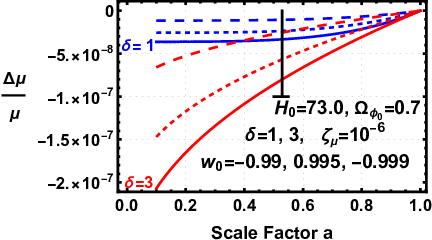
The cases represent the least evolution and the cases represent the most evolution with the lying between the two. All of the cases satisfy the constraint, mainly because of the small deviations of from minus one. Only a small tightening of the constraint would start to eliminate some of the cases. The proposed fiducial case of and is well within the observational constraint. Additionally restrictive observational constraints can always be cosmologically accommodated by making closer to minus one or by lowering the value of the particle physics parameter .
The last sentence in the above paragraph indicates that a constraint on the temporal variance of either or is a constraint on a cosmology-particle physics plane defined by and . An earlier analysis (Thompson 2013) determined the relationship between and as
| (49) |
where is the scale factor of the observation. Equation 19 for is the source of the term in equation 49. Equation 49 defines regions in the - plane that satisfy the observational constraint and those that don’t. Figure 17 shows the allowed and forbidden area for the constraint.

The positive and negative tracks for each case are due to the positive and negative values for in equation 49. The more restricted allowed area is due to the greater evolution of . as shown in figure 16, that requires a smaller to meet the constraint than the case. The CDM point in the figure is the 0,0, origin where and . A confirmed observation of with no detected variance of would place a hard limit on the particle physics parameter but also would require new physics to account for a deviation of from minus one.
19 Conclusions
This study addresses the question of whether dark energy is static or dynamic by first pointing out that the use of parameterizations to represent dynamical cosmologies results in not only erroneous likelihoods but also in erroneous conclusions about the validity of dynamical cosmologies such as quintessence. The study then presents a methodology for creating accurate analytic templates of the evolution of cosmological parameters and fundamental constants for the flat quintessence dynamical cosmology. The methodology utilizes a modified beta function formalism to determine the evolution of the quintessence scalar as a function of the observable scale factor. Solutions for the evolution of parameters and constants that were previously only functions of the unobservable scalar are then translated to templates that are functions of the scale factor for direct comparison with the current and expected cosmological observations. Recognizing that dynamical cosmologies can have a multitude of dark energy potentials the study introduced the concept of Specific Cosmology and Potential, SCP, templates to replace the parameterizations with SCP evolutionary templates based on the physics of the cosmology and dark energy potential.For this reason the study concentrated on the methodology to produce SCP templates that can embrace a broad range of analytic physics based potentials..
To demonstrate the formalism the study then calculated SCP templates of several observable and some necessary but not observable parameters such as the time derivative of the scalar that appear in the functions of many observable parameters. An important aspect of the study is the example quartic polynomial dark energy HI potential. The modified beta function formalism applied to flat quintessence with the HI potential resulted in a scalar that is a simple function of the Lambert W function. This step provided the means to produce accurate analytic SCP templates as a function of the scale factor.
Given the many observational successes of the CDM static cosmology the study chose boundary conditions close to CDM. In particular values close to, but not equal to, minus one were adopted. This choice produced a simplification of the beta function formalism where the beta function for quintessence is the negative of the logarithmic derivative of a slightly modified dark energy density. The beta function is then accurately approximated by the logarithmic derivative of the potential. Care should be taken in using the formalism for values significantly different than minus one. Equation 7 shows that the kinetic term is directly proportional to . If becomes too large the approximation can break down and other means must be employed. The SCP templates are calculated by imposing the Friedmann constraints on the parameters. Since the studied epoch included only the matter dominated and dark energy dominated epochs, radiation is not included in the calculations. This precludes utilization of the templates for scale factors smaller than 0.016, such as the CMB dominated epoch, that have significant radiation densities.
The polynomial HI potential provided a significantly larger range of evolutions than the often use monomial potentials. In particular small changes of the constant term in the potential produced dark energy EoS evolution that were both freezing and thawing plus evolutions that transitioned from freezing to thawing. Giving the naturalness of the HI potential and the large range of evolutions the study suggests that the HI SCP templates become a fiducial dynamical cosmology in the same way as CDM is for static cosmologies. Several of the cases studied are indistinguishable from CDM with the accuracy of the present and near future observations even though their dark energy density arises from a dynamical scalar field rather than a cosmological constant. Given this and the relative rigidity of the predicted evolutions it appears that CDM is easy to falsify but hard to confirm and that flat HI quintessence is hard to falsify but easy to confirm if new observations confirm predictions such as a dynamical dark energy EoS.
The study concluded with an examination of the role of fundamental constants in the discrimination between static and dynamical cosmologies. The scalar in a dynamical dark energy that interacts with gravity will most likely interact with other sectors which produces temporal variations in the fundamental constants. To date no confirmed variations of either or have been found at the one part in level. All of the cases in this study predict variations that are less than the current limits. Future observations may, however, lower the limit that would make it difficult to meet the constraints or find a variation that is consistent with the dynamical predictions.
20 Appendix 1, Flat HI quintessence abridged templates
This is an abridged set of evolutionary templates for flat HI quintessence. The unabridged template set contains significantly more information including code for implementing the templates. The templates developed in the main text are gathered here to provide a convenient listing for community use. The appendix repeats information provided in the text to gather most of the relevant material in a single location.
Units: Natural units are utilized with , , and set to one. The units of mass are the reduced Planck mass .
General constants: The constant . In the mass units utilized here but it is retained to provide the proper mass units for the templates.
Primary variable: The primary variable is the scale factor . All templates are functions of the observable scale factor.
Special functions: The Lambert W function is used extensively in the templates. See (Olver, F. W. F., Lozier, D. W., Boisvert, R.F., and Clark, C.W 2010) for a comprehensive description of the function.
The Ratra-Peebles, RP scalar: The RP scalar is used in all of the templates. Its functional from is
in terms of the Lambert W function with and as constants given below.
The Higgs Inspired, HI, dark energy potential: The dark energy potential is
where is a constant with units of mass in . The constant also has units of . Both and
will be repeated below along with the definitions of the constants , and .
Assigned constants: The HI potential constant is assigned the constants 1.0, 2.0, and 3.0 in this work
Changeable cosmological constants: These constants are assigned values in this work and appear in the templates, thus they can be assigned different values according the the desired boundary conditions for the cosmological parameters. The boundary conditions are set at the current epoch hence the subscript 0 on their designations.
the Hubble parameter
The dark energy equation of state
Cosmological parameter templates: The cosmological parameter template formats include, where possible, the parameter first in terms of the RP scalar , second the parameter in terms of the Lambert W function, third its magnitude at a scale factor of one for , and and fourth any associated constants.
The Ratra Peebles scalar
The beta function
The dark energy potential
The Hubble parameter
The derivative of the scalar with respect to the scale factor
The derivative of the scalar with respect to time
The kinetic term X =
The dark energy density
The matter density
is not a function of
The dark energy pressure
The dark energy equation of state
21 Referrences
References
- (2022) Thompson, R.I. 2022, ”Dynamical templates for comparison to Lambda CDM: Static or dynamical dark energy?”, 2022arXiv220401863v1 ,2022
- National Academies of Sciences, Engineering, and Medicine (2021) Committee for a Decadal Survey on Astronomy and Astrophysics 2020 (Astro2020) Pathways to Discovery in Astronomy and Astrophysics for the 2020s, 2-22 (The National Academies Press, Washington, DC)
- Scherrer and Sen (2008) Scherrer, R. J., and Sen, A.A., 2008, “Thawing quintessence with a nearly flat potential”, Physical Review D. 77, 083515 2008
- Copeland (2006) Copeland, E. J., Sami, M. and Tsujikawa, S. Dynamics of dark energyJ. Mod. Phys. D, 15, (2006),1753–1936.
- Cicciarella and Pieroni (2017) Cicciarella, F. and Pieroni, M. 2017, “Universality for quintessence”, Journal of Cosmology and Astroparticle Physics, 1708, no. 8, 010 -039
- (2018) Bahamonde, S., Bohmer, C.G., Carloni, S., Copeland, E.J., Fang, W. and Tamanini, N. 2018, “Dynamical systems applied to cosmology: Dark energy and modified gravity”, Physics Reports, 775-777, 1-122.
- Carroll (1998) Carroll, S. M., Quintessence and the rest of the world: Suppressing long-range interactions, Phys. Rev., Lett., 81 (1998), 3067, [arXiv:astro-ph/9806099]
- Coc (2007) Coc, A., Nunes,N., Olive, K.A., Uzan, J-P, and Vangioni, E., Coupled variations of fundamental constants and primordial nucleosynthesis, Phys. Rev. D 76 (2007) 023511, [astro-ph/0610733]
- Chevallirer (2001) Chevallier, M. and Polarski, D. 2001, “Accelerating universes with scaling dark matter”,International Journal of Modern Physics D, 10, 213-224
- Linder. (2003) Linder, E.V. 2003.”Exploring the expansion history of the universe”, Physical Review Letters, 90, 091301
- Vikman (2005) Vikman, A. 2005 “ Can dark energy evolve to the phantom?, Physics Review, D 71, 023515.
- Planck Collaboration (2019) Planck Collaboration: Aghanim, N., Akrami,Y., Ashdown, M. Aumont, J. Baccigalupi, C. Ballardini, M., Banday, A. J., Barreiro, V, Bartolo, N., Basak, S., Battye, R., Benabed, K., Bernard, J.-P., Bersanelli, M. , Bielewicz, P. J., Bock, J., Bond, J. R., Borrill, J., Bouchet, F. R., Boulanger, F., Bucher, M., Burigana, C., Butler, R. C., Calabrese, E. Cardoso, J.-F., Carron, J., Challinor, A., Chiang, H. C., Chlub, J., Colombo, L. P. L., Combet, C., Contreras,D., Crill, B. P., Cuttaia, F., de Bernardis, V, de Zotti, G, Delabrouille, J., Deloui, J.-M., Di Valentino, E., Diego, J. M. Dore6, O., Douspis, M., Ducout, A., Dupac, X., Dusini, S. Efstathiou, G., Elsner, F. Enßlin, T. A., Eriksen, H. K., Fantaye, Y., Farhang, M. Fergusson, J., Fernandez-Cobos, R., Finelli, F., Forastieri, F., Frailis, M., Fraisse, A. A. Franceschi, E., Frolov, A., Galeotta, S., Galli, S., Ganga, K., Genova-Santos, R. T., Gerbino, M., Ghosh, Gonzalez-Nuevo, T. J., Gorski, K. M., Gratton, S., Gruppuso, A., Gudmundsson, J. E., Hamann, J., Handley, W., Hansen, F. K., Herranz, D., Hildebrandt, S. R., Hivon, E., Huang, Z., Jones, W. C., Karakci, A., Keihanen, E., Keskitalo, R., Kiiveri, K., Ki2 J., Kisner, T. S., Knox, L., Krachmalnico, N., Kunz, M., Kurki-Suonio, H., Lagache, G., Lamarre, J.-M., Lasenby, A., Lattanzi, M., Lawrence, C. R., Le Jeune, M., Lemos, P., Lesgourgues, J., Levrier, F., Lewis, A., Liguori, M., Lilje, P. B., Lilley, M., Lindholm, V., Lopez-Caniego, M., Lubin, P. M. Ma, Y.-Z., Macas-Perez, J. F., Maggio, G., Maino, D., Mandolesi, N., Mangilli, A., Marcos-Caballero, A., Maris, M., Martin, P. G., Martinelli, M., Martnez-Gonzalez, E., Matarrese, S., Mauri, N., McEwen, J. D., Meinhold, P. R., Melchiorri, A., Mennella, A., Migliaccio, M., Millea, M., Mitra, S., Miville-Deschˆenes, M.-A., Molinari, D., Montier, Morgante, L. G., Moss, A., Natoli, P., Nørgaard-Nielsen, H. U., Pagano, L., Paoletti, D., Partridge, B., Patanchon, G., Peiris, H. V., Perrotta, F., Pettorino, V., Piacentini, F., Polastri, L., Polenta, G., Puget, J.-L., J. P. Rachen18, M. Reinecke72, M. Remazeilles64, Renzi, A., Rocha, G., Rosset, C., Roudier, G., Rubi˜no-Mart60, J. A., Ruiz-Granados, B., Salvati, L., Sandri, M., Savelainen, M., Scott, D., Shellard, E. P. S., Sirignano, Sirri, G., Spencer, L. D., Sunyaev, R., Suur-Uski, A.-S. , Tauber, J. A., Tavagnacco, D., Tenti, M., Toffolatti, L., Tomasi, M., Trombetti, T., Valenziano, L., Valiviita, J., Van Tent, B., Vibert, L., Vielva, P., Villa, F., Vittorio, N. Wandelt, B. D., Wehus, I. K., White, M., White, S. D. M., Zacchei, A., and Zonca, A. 2019 “Planck 2018 results. VI. Cosmological parameters “,arXiv:1807.06209v2 [astro-ph.CO] 20 Sep 2019
- Di Valentino, Melchiorri and Silk (2020) Di Valentino E., Melchiorri, A and Silk, J. 2020, ‘Cosmological constraints in extended parameter space from the Planck 2018 Legacy relase”, Journal of Cosmology and Astroparticle Physics, 01, 013, 1-13
- Di Valentino (2020) Di Valentino E. 2020, “A (brave) combined analysis of the Ho late time direct measurements and the impact on the Dark Energy sector”, arXib:2011.0024v1 [astro-ph.CO] 31 Oct. 2020
- Riess et al. (2022) Riess, A.G., Yuan, W., Marci, L.M., Scolnic, D., Brout, D., Casertano, S., Jones, D.O., Murakami, Y., Breuval, L., Brink, T.G., Filippenko, A.V., Hoffjann, S., Jha, S.W., Kenworthy, W.D., Mackenty, J., Stahl, B.E. and Zheng, W., A Comprehensive Measurement of the Local Value of the Hubble Constant with 1 km s Mpc Uncertainty from the Hubble Space Telescope and the SH0ES Team, ApJL 934 (2021). L7 59, arXiv:2112.04510v2
- Ratra and Peebles (1988) Ratra, B and Peebles, P. J. E.. 1988, “Cosmological consequences of a rolling homogeneous scalar field” Physical Review D 37,12, 3406.
- Peebles and Ratra (1988) Peebles, P. J. E. and Ratra,B. 1988, “Cosmology with a Time-Variable Cosmological ”Constant””, The Astrophysical Journal Letters, 325, L17
- Binetruy et al. (2015) Binetruy, P., Kiritsis, E., Mabillard, J. . Pieroni, M. & Rosset, C. 2015 “Universality classes for models of inflation”, Journal of Cosmology and Astroparticle Physics, 1504, no. 04, 033-64
- Binetruy, Mabillard Pieroni (2017) Binetruy, P., Mabillard, J. and Pieroni, M. 2017, “Universality in generalized models of inflation”, Journal of Cosmology and Astroparticle Physics, 060, 1-19
- Kohri and Matsui (2017) Kohri, K. and Matsui H., 2017, “Cosmological Constant Problem and Renormalized Vacuum Energy Density in Curved Background”, Journal of Cosmology and Astroparticle Physics, 06, 006
- Olver, F. W. F., Lozier, D. W., Boisvert, R.F., and Clark, C.W (2010) Olver, F. W. F., Lozier, D. W., Boisvert, R.F., and Clark, C.W 2010, in NIST Handbook of Mathematical Functions, Chap. 4, p. 111, 1st ed, (Cambridge University Press, New York)
- Dahiya (2022) Dhiya, D. and Jain, D., 2022 ”Revisting the epoch of cosmic acceleration” 2022 arXiv:2212.04751v2 [astro-ph.CO]
- Murphy (2021) Murphy, M. et. al. Fundamental physics with ESPRESSO: Precise limit on variations in the fine-structure constant towards the bright quasar HE 0515-4414, (2021), arXiv:2112.05819v1
- Bagdonaite (2013) Bagdonaite, J., Dapra‘, M., Jansen,P., Bethlem, H. L., Ubachs, W., Muller, S., Henkel, C. and Menten, K. M. Robust Constraint on a Drifting Proton-to-Electron Mass Ratio at z = 0:89 from Methanol Observation at Three Radio Telescopes Phys. Rev. Let. 111, (2013) 231101, arXiv:1311.3438
- Kanekar (2015) Kanekar, N., Ubachs, W., Menten, K. M., Bagdonaite, J., Brunthaler, A., Henkel, C., Muller, S., Bethlem, H.L., and Dapra, M. Constraints on changes in the proton–electron mass ratio using methanol lines MNRAS, 448, (2015), L104, arXiv:1412.7757
- Thompson (2013) Thompson, R.I., Constraining cosmologies with fundamental constants - I. Quintessence andK-essence, MNRAS 428, (2013), 2232, arXiv:1210.3031