Differential Convolutional Fuzzy Time Series Forecasting
Abstract
Fuzzy time series forecasting (FTSF) is a typical forecasting method with wide application. Traditional FTSF is regarded as an expert system which leads to loss of the ability to recognize undefined features. The mentioned is the main reason for poor forecasting with FTSF. To solve the problem, the proposed model Differential Fuzzy Convolutional Neural Network (DFCNN) utilizes a convolution neural network to re-implement FTSF with learnable ability. DFCNN is capable of recognizing potential information and improving forecasting accuracy. Thanks to the learnable ability of the neural network, the length of fuzzy rules established in FTSF is expended to an arbitrary length that the expert is not able to handle by the expert system. At the same time, FTSF usually cannot achieve satisfactory performance of non-stationary time series due to the trend of non-stationary time series. The trend of non-stationary time series causes the fuzzy set established by FTSF to be invalid and causes the forecasting to fail. DFCNN utilizes the Difference algorithm to weaken the non-stationary of time series so that DFCNN can forecast the non-stationary time series with a low error that FTSF cannot forecast in satisfactory performance. After the mass of experiments, DFCNN has an excellent prediction effect, which is ahead of the existing FTSF and common time series forecasting algorithms. Finally, DFCNN provides further ideas for improving FTSF and holds continued research value.
Index Terms:
Fuzzy Time Series, Forecasting, Deep Learning, Convolutional Neural NetworkI Introduction
Time series is a common data type, with univariable and multivariable sub-types. There are also many research directions of time series, such as time series clustering [1, 2, 3], anomaly detection [4, 5], time series entropy [6, 7], time series forecasting [8, 9, 2] and so on [10]. Time series forecasting has attracted the attention of many scholars and experts. Time series forecasting is useful in a wide range of fields, such as stock forecasting [11], wind forecasting, population forecasting and so on. At present, there are many forecasting methods, such as the common statistical methods including exponential smoothing (ETS) model [12] and Holt-Winter ETS model [13], autoregression (AR) [14], moving average model (ARIMA) [15] and seasonal ARIMA model [16]. However, the forecasting accuracy of the common model is not enough to meet needs currently. In order to improve the accuracy of forecasting, increasingly novel and advanced methods have been developed, such as the method based on machine learning [17], neural network [18] and complex network. How to further improve the accuracy of time series forecasting is an open problem.
Fuzzy time series forecasting (FTSF) is a far-reaching time series method based on fuzzy theory. Fuzzy theory has the ability to deal with the uncertainty of data. It is widely used in engineering practice, such as game theory [19, 20, 21], intelligent decision-making [22, 23, 24, 25], information fusion [26, 27], data classification [28, 29, 30], bioinformatics [31, 32], pattern classification [33, 34] and so on [35, 36]. The previous FTSF works have a common fact that the process of fuzzifying a variable and the process of defuzzifying a variable must be certain. Furthermore, there is only reasoning between fuzzy variables which leads to a high possibility of prediction bias due to fuzzy set creation. In addition, due to reasoning among the mass of fuzzy rules, reasoning as a expert system is not an optimal way that there are potential differences and inherent relations. Besides, the length of fuzzy reasoning is also limited by the mode of the expert system, since the expert system is not able to learn pattern of longer fuzzy rules. Therefore, it is proper to utilize optimization algorithm to further reasoning. One of the implementations of the optimization algorithm is the neural network.
Stationary is a crucial feature of time series, and time series are usually non-stationary due to trend and so on. According to the method of Cleveland et al. [37], time series can be decomposed into residuals component, seasonal component and trend component. Because of the trend component, the tendency of a time series to change in one direction over time. As mentioned above, FTSF can only reason about fuzzy variables. When the time is far from the time when the fuzzy system is established, the variables will be fuzzified to first or last fuzzy set of the previously established fuzzy set because of the accumulated trend. Then, each time will be regarded as the same fuzzy variable and defuzzifying process leads to the same forecasting output which called fuzzy failure (FF). To solve FF problem, on the one hand, the time series need to remove the trend, and on the other hand the expert system approach needs to be replaced, because expert systems lacks knowledge summarization and autonomous learning capabilities.
To solve the mentioned problem, Differential Fuzzy Convolutional Neural Network (DFCNN) is proposed. In DFCNN, the data are differenced, which is an effective method to remove time series trends. To solve the problem that the expert system can only reason about fuzzy variables, the DFCNN utilizes the neural network to optimize the FTS. Recently, some works proposed FTSF with Artificial Neutral Network (ANN) [38, 39, 40, 41, 42]. FTSF with ANN is limited by the optimization object of ANN fuzzy variables [43, 44, 45, 46, 47]. Compared with the combined FTS and ANN approach, the proposed method skips the establishment of fuzzy sets, making the inference not limited to fuzzy variables. Proposed Fuzzy Generator with reference to the fuzzy treatment of traditional FTS prediction methods. Fuzzy Generator divides the fuzzy interval with the construction of coding theory, which makes the input time series expand into Fuzzy Token. Fuzzy Token is a type of vector remained the full information of converting time series to fuzzy variables. The convolutional layer is a mechanism used to replace the membership functions while making the inference not limited to fuzzy variables. For the problem of the length of fuzzy inference, Sliding Window algorithm is applied in DFCNN to process the data, and the window size is equivalent to the length of the fuzzy rules of traditional FTS. By processing the convolutional layer, DFCNN can handle fuzzy rules that are not restricted to the previous binary fuzzy rules and can build longer fuzzy inference. So the contribution of this work is as follows:
- •
Proposing Fuzzy Generator solves the limitation of fuzzifying variables.
- •
Utilizing the Convolution layer as membership functions solves the limitation of expert system.
- •
Utilizing the Sliding Windows algorithm expands the limitation of length of fuzzy rules.
In the experimental section, many FTSF methods are selected to be compared methods. To avoid the effect of trend, each compared method was appended the Difference algorithm. In terms of prediction error, DFCNN exceeds the comparison method. DFCNN is also compared with common time series forecasting methods. In the vast majority of cases, the predictive performance of DFCNN is stable. However, in one of the small datasets DFCNN is not able to achieve the most accurate prediction. The limitations of DFCNN are analyzed in this dataset, as well as for the prediction errors of the comparison methods. Meanwhile, the effects of the number of convolutional kernels and window size on DFCNN predictions were experimented. The window size directly affects the prediction accuracy and does not show a significant correlation with the selected data and correlation, and the prediction is relatively stable under the default parameters. In a word, the experimental results demonstrate that the comprehensive prediction error of DFCNN is low, which is better than the comparison methods.
The structure of the article is as follows. In the second section, it explains the previous methods and problems of fuzzy time series forecasting. In the third section, the basic theory of the proposed method is introduced. In the fourth section, the article proposes DFCNN. In the fifth section, the article shows the experimental effect of DFCNN and the comparison and analysis with traditional fuzzy time series forecasting. In the sixth section, the article summarizes the full text and looks forward to future work.
II Previous Fuzzy Time forecasting Research and Problems
Fuzzy time series forecasting is a common method in time forecasting. The initial fuzzy time series was used for enrollment forecasting of University of Alabama [48]. The data size of the previous experiments was small, and in this case, the pure use of fuzzy logic can effectively predict future enrollment. In today’s era of mega data, it is possible to meet FF problems when use FTSF algorithm.
II-A Process of fuzzy time series forecasting
First assume that the time series is T, and T is defined in Eq.1:
| (1) |
where is the time of time node , is the value of time node and is the size of time series .
Taking Chen’s methods [48] as an example, the fuzzy time series forecasting method usually adopts the following steps:
- 1.
An interval of a time series is defined so that the maximum values and minimum values of the time series belong to this interval as Eq.2. is an arbitrary positive number.
(2) - 2.
According to the proposed method, the interval is divided into some sub-intervals . The number of divisions is an arbitrary positive number.
- 3.
Establish fuzzy sets . The establishment of the fuzzy set and the interval established in the second step are related by the membership function.
- 4.
Fuzzify time series into fuzzy linguistic variable series .
- 5.
The inference system is built by forming fuzzy rules from two consecutive linguistic variables in the fuzzy linguistic variable series.
- 6.
Assume current time is . Fuzzy current time value into corresponding fuzzy linguistic variable . According the existed fuzzy rules, inference system generates a certain fuzzy rule .
- 7.
Defuzzify into and output .
II-B Existing problems
II-B1 Limitation of fuzzy reasoning
According to the forecasting process of fuzzy time series, the input of fuzzy time series forecasting is the current time node and the fuzzy set to which the current node belongs. The fuzzy set can be defined by membership functions and intervals . The membership function belongs to the process of fuzzy time series forecasting, and the input of the fuzzy time series forecasting is the time node and the interval to which the time point belongs.
The forecasting method of fuzzy time series can be transformed as a function ”Fuzzy Time Series Forecasting” () in Eq.3, Eq.4.
| (3) |
| (4) |
where are the left and right boundaries of interval .
The flow chart of FTSF is left side of Fig.1. It means that the fuzzy inference logic of FTSF is independent of the original data directly. It is also a limitation of expert system which is unable to learning data feature by itself. Also there are some FTSF methods based on ANN, and fuzzy inference is improved. But FTSF methods based on ANN is not able to solve the improper process when fuzzy sets is establishing.
II-B2 Fuzzy failure
FF problem is mentioned. Different time series have different properties, such as periodicity and trend. Chen’s method was an example of FTSF and forecast the Association of Securities Dealers Automated Quotations (NASDAQ) average [48] in Fig.2. There is a FF problem. Each time is regarded as the same fuzzy variable and the same defuzzifying process then output the same result.
II-B3 Limitation of length of fuzzy rules
When FTSF method fit to an existed time series need to generate many fuzzy roles like . It is base of fuzzy inference and defuzzifying. But there is no reason not to consider how to process fuzzy rules which length is large than 2. Arbitrary positive number large than 2 is a possible length of fuzzy rules, but FTSF is an expert system method which means it need to proposed certain reasoning logics for each arbitrary positive number.
III Preliminary
III-A Difference algorithm
The difference algorithm takes the difference between each time node in the time series , while retaining the value of the first time node as Eq.5 .
| (5) |
The difference series effectively removes the trend of the time series, and the initial value of the time series is recorded. If you restore the original time series, it only need to add the difference subseries values before each node.
III-B Convolution
In deep learning, convolution operation is a common operation for feature mapping [49]. Now suppose the input of the convolution operation is and the kernel function is . The convolution operation is usually denoted by the symbol . The output of the convolution operation is denoted as in Eq6, Eq.7.
| (6) |
| (7) |
Where , , are in matrix form. The convolution operation will continuously update the weight of the kernel function after supervised learning and multiple cashback propagation, and finally output the features of the map. If is a vector, the output of the convolution is calculated according to Eq.8.
| (8) |
IV Differential Fuzzy Convolutional Neural Network
A time series is assumed.
IV-A Difference Layer
The sequence obtained after differencing the time series is called as Eq.5.
Difference Layer is capable of removing the trend and time series is more stationary. The first value of time series needs to reserve for recover the original time series from difference series.
IV-B Sliding Window Layer
The formula for sliding window algorithm is Eq.9, where refers to the i-th result of the sliding window and is the original input.
| (9) |
Suppose that the two adjacent values of the original time series are and . The fuzzy variable corresponding to is and the fuzzy variable corresponding to is . So the resulting fuzzy rule is . When , Sliding Windows algorithm’s first output is which is equivalent to defuzzified .
Suppose the value of the original time series after is . The fuzzy variable corresponding to is . Then the fuzzy rule becomes . When , Sliding Windows algorithm’s first output is which is equivalent to defuzzified .
There is no good way to deal with fuzzy rules which length is over 2 and make forecastings based on fuzzy rules. Sliding Windows algorithm slove the problem of limitation of fuzzy rules’ length. But Silding Windows algorithm is not able to consider any information of original fuzzy sets. So Fuzzy Generator is a way to embed the necessary information of establishing fuzzy set instead of create fuzzy sets and fuzzy variables directly.
IV-C Fuzzy Generator Layer
Definition 1
Encoding Partition
For a given fuzzy interval , assuming corresponding time series length is , then the number of divided fuzzy interval is . The fuzzy intervals boundaries set is shown in Eq.10. The partitioned fuzzy intervals are all of equal length.
| (10) |
Here is the proof of this definition. Suppose the fuzzy set membership is either 1 or 0 in Eq.11.
| (11) |
where is the membership function of arbitrary fuzzy set and is the i-th time node in time series .
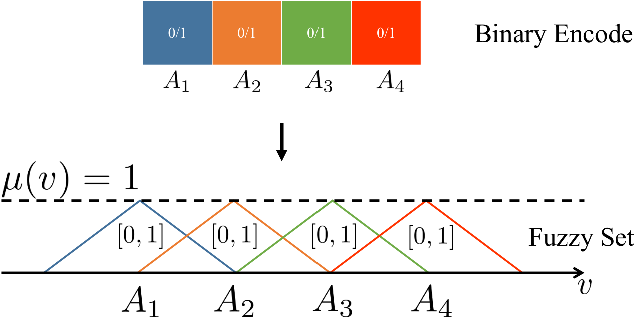
Then if fuzzy sets needs to be used to encode a time series of length bits, the required number of fuzzy sets is calculated in Eq.12, Eq.13, Eq.14:
| (12) |
| (13) |
| (14) |
This method of calculating the number of fuzzy sets is the same as that of binary encoding [50]. However, the membership function of a fuzzy set is a continuous map. The original fuzzy set is used as a bit, which can represent more states. Fig.3 shows an example of partitioning fuzzy sets by coding ideas. Therefore, the number of fuzzy intervals is split according to , which is able to fully encode all the nodes in the time series.
Example Assume a time series T in Eq.15
| (15) |
where is composed of time points . The number of fuzzy intervals in Eq.16 required for the time series is
| (16) |
According to Eq.16, the resulting fuzzy set is assumed to be three equally long fuzzy intervals .
| (17) |
| (18) |
| (19) |
Domain is defined in Eq.17, Eq.18, Eq.19 which refer to the minimum value in time series values, also refer to the maximum value and refer to standard deviation. The quantity of partial coincident fuzzy intervals is in Eq.20 that the length of the time series is reduced to due to Differential Layer. The interval is then divided into uncoincident segments of equal length. There are boundaries for these equally long intervals, and the set of boundaries is denoted by in Eq.21 as Fig.4.
| (20) |
| (21) |

Definition 2
Fuzzy Token
Fuzzy Token is a vector contains the information of establishing fuzzy set and fuzzy variable. The nearest fuzzy intervals boundaries of time series values are embedded into Fuzzy Token. The formula of Fuzzy Token is Eq.22, Eq.23 and Eq.24.
| (22) |
| (23) |
| (24) |
Time series value is converted into the Fuzzy Token which are the two nearest boundaries in fuzzy intervals boundary set mentioned by Fuzzy Generator. The definition of and is shown in Eq.23, Eq.24. and has two cases to be defined shown in Fig.5. If time series value is in the boundary set , for , generating Fuzzy Token ignores in and also find the nearest two boundaries.

IV-D Batch Norm Layer
For the Fuzzy Token , it is a optimal to normalize as Eq.26 [51, 52] which is able to accelerate the process of learning process. The mean and standard-deviation are calculated. and are learnable parameter vectors of size which is the number of features or channels of the input. The normalized Fuzzy Token is written as .
| (25) |
IV-E Convolution Layer
Fuzzy Generator combines the value of traditional fuzzy variable, and convolution operation can be used as a type of fuzzy function. Convolution Layer is a one-dimensional Convolution Layer which is equivalent to membership function with learning parameter weight and bias .
| (26) |
| (27) |
| (28) |
Fuzzy variable is determined membership function which is determined by fuzzy interval and membership function in FTSF. Eq.26, Eq.27 and Eq.28 is common membership functions of fuzzy sets. Assume is the boundaries of corresponding fuzzy set . For a fuzzy intervals like , the membership function of is Eq.29.
| (29) |
is a constant variable. To optimal fit to input time series, needs to be treat as a learnable parameter . is same as the left and right boundaries in Fuzzy Token. So one dimension Convolution Layer is equivalent mechanism of fuzzy variables.
Because of the sliding window, the length of the input for the convolution layer is , where the number of channels is and feature size is 3. The convolution layer has a parameters, the number of output channels of the convolution , which is also the number of convolution kernels. The number of convolution kernels can be set to multiple and is usually set to 2. Multiple convolution kernels can increase the robustness of the network. Convolution kernel size is , and convolution kernel sums the all channel which gathers information of fuzzy rules in Eq.30. And the length of equivalent fuzzy rule is not limited.
| (30) |
In right side of Fig.1, Fuzzy Generator and Convolution layer is separated in fuzzy information extraction block. It is different to FTSF’s Fuzzifying process based on expert system for Fuzzy Generator and Convolution layer that the relevant learnable parameter helps fit the input time series further.
IV-F Linear Layer
To predict the next time point, in FTSF, the fuzzy rules should be weighted according to the existing fuzzy rules and output. The output of the convolution is summed and the final forecasting is made through the linear layer. Assuming the output of the convolution layer is , the last dimension needs to added weight and sum up. Similar to FTSF, linear layer adopts a weighted way to predict the previously created fuzzy rules in Eq.31. The overall structure of the network is shown in Fig.6.
| (31) |
In left side of Fig.1, in the fuzzy inference and forecasting block, traditional FTSF’s defuzzifying process is based on expert system. Also FTS with ANN utilize ANN to output the proper label of target fuzzy set and use same method as traditional FTSF to defuzzyify. In essence, FTS with ANN does not have enough learning ability.
IV-G Recovery
The target of Linear Layer is difference series . The recovery process is necessary for output in Eq.32.
| (32) |
is origin time series of previous one time step of . In the same way as the FTSF, DFCNN is a single step forecasting method due to Recovery mechanism. To keep stationary, Difference algorithm is applied in DFCNN also leads to single step forecasting. If Difference algorithm is replaced by other algorithm which transforms time series to stationary time series and does not rely on one time step values, the multistep forecasting can be implemented.

V Experiment and Analysis
The datasets used in the experiment are M competition dataset and Construction Cost Index (CCI). Involved in the experiment compared methods from forecastingdata.org. The experimental environment is AMD Ryzen 7950X (Cores: 16, Base Clock: 4.5GHz), RTX3090 (24GB) and the RAM is 64GB.
V-A Datasets
The experiments involve 5 datasets with different sizes and types.
Dataset 1: Construction Cost Index
- •
Description: The Construction Cost Index (CCI) is published once a month by Engineering Cost Record (ENR) [53]. For the purpose of forecasting time series, 295 CCI data values (CCI data sets from January 1990 to July 2014) were employed. In the experiment, CCI divided the time series into training data sets and forecasting data sets in an 8:2 ratio.
- •
Intention: CCI data set is a single time series which is a typical non-stationary time series with significant trend. Fig.7 shows the trend of CCI test part. CCI data sets can verify the validity of DFCNN for non-stationary time series. In Fig.7, traditional FTS methods failed to forecast.

Fig. 7: Trend of CCI dataset and comparative results
Dataset 2-5: Makridakis Competition
- •
Description of M Competition: Makridakis Competition is also known as M Competition. The M Competition is an open competition to evaluate the accuracy of different time series forecasting methods. So M Competition can be used as a benchmark test of the effect of time series forecasting method.
- •
Dataset 2: M1 Competition The first M Competition provided 1001 time series which is not real-time time series.
- •
Dataset 3: M2 Competition The second M Competition provided 29 time series which is real-time time series come from many collaborating organizations and competition announced in advance.
- •
Dataset 4: M3 Competition The third M Competition provided 3003 time series which were in the following domains: micro, industry, macro, finance, demographic, and other.The frequencies of time series include yearly, quarterly, monthly, daily, and other.
- •
Dataset 5: M4 Competition The fourth M Competition provided 100000 time series which were in the following domains: micro, industry, macro, finance, demographic, and other. The frequencies of time series include yearly, quarterly, monthly, weekly, daily, and hourly.
TABLE I: M Dataset Features Dataset Quantity Number Min Max Horizion M1 Yearly 181 15 58 6 Quarterly 203 18 114 8 Monthly 617 48 150 18 Total 1001 M2 Quarterly 12 163 167 5 Monthly1 42 33 94 14 Monthly2 4 213 225 15 Total 60 M3 Yearly 645 20 47 6 Quarterly 756 24 72 8 Monthly 1428 66 144 18 Other 174 71 104 8 Total 3003 M4 Yearly 23000 19 841 6 Quarterly 24000 24 874 8 Monthly 48000 60 2812 18 Weekly 359 93 2610 13 Daily 4227 107 9933 14 Hourly 414 748 1008 48 Total 100000 - •
Statistical characteristics: Each M Competition specifies different forecast horizons for different frequency time series, in order to ensure that each prediction method has the same prediction interval. The maximum length of time series in M4 is even longer than 8000 time points which is a huge challenge for single step forecasting methods (include DFCNN and traditional FTS methods). Simultaneously, there is a large margin between minimum and maximum length of M datasets which evaluates the capability of time series forecasting algorithms to extract predictive features from time series of varying lengths.
- •
Intention: M Competition datasets is involved by Monash Time Series Forecasting Repository (https://forecastingdata.org/) which mentioned in the comparison model section and is an open source containing time series data set to assess benchmark [54]. M Competition datasets and Monash repository guarantee the fairness of the data and the comprehensiveness of the evaluation of the time series forecasting algorithm.
V-B Comparative Models
In order to demonstrate the accuracy of the proposed model, the comparative models are divided into two categories: fuzzy time series forecasting method and Monash benchmark method.
Fuzzy time series forecasting method:
Comparative FTSF methods demonstrate the improvement of DFCNN on previous work. In order to verify the advantages of DFCNN fairly, the comparative models is representative backbone works of FTSF because DFCNN is a novel FTSF method and also a backbone work.
- •
First Order Conventional FTS method (FOCFTS) [48] is a basic method that transforms the crisp historical data into fuzzy sets based on predefined linguistic variables, establishes fuzzy logical relationships between the fuzzy sets, and converts the fuzzy forecasted values.
- •
Trend Weighted FTS method (TWFTS) [55] extends the First Order Conventional FTS method by incorporating trend analysis. It detects the direction and magnitude of the changes in the historical data and assigns trend weights to the fuzzy sets and rules.
- •
High Order Interval FTS method (HOIFTS) [56] extends the First Order Conventional FTS method by incorporating weight algorithm and high order FTS algorithm. It utilized a group of continuous fuzzy logic relationships as input of FTSF algorithm and applied the weight algorithm to improve forecasting accuracy.
- •
FTS with ANN (FTSWA) [43] extends the First Order Conventional FTS method by determining fuzzy relationships by Artificial Neural Networks (ANN). After establishing the fuzzy sets, ANN processed the fuzzy relationships which solved the problem that observations of time series are defined linguistically or do not follow the assumptions required for time series theory.
A more intuitive difference between DFCNN and the comparative models is shown in Tab.2.
| Model | Weighted | Learnable | Non-stationary | Expanded-Relationship | Differences with DFCNN |
| FOCFTS | Same as below | ||||
| TWFTS | ✓ | DFCNN uses differences algorithm to remove trends | |||
| HOIFTS | ✓ | ✓ | DFCNN extends the length of fuzzy relationships | ||
| FTSWA | ✓ | DFCNN learns before establishing fuzzy sets | |||
| DFCNN | ✓ | ✓ | ✓ | ✓ | - |
The Monash Time Series Forecasting Benchmark is aimed to compare common models of DFCNN and non-FTS with M Competiton datasets. These include statistical models such as Auto-Regressive Integrated Moving Average, machine learning models such as CatBoost, deep learning models such as Transformer and so on.
Monash Time Series Forecasting Benchmark:
- •
Exponential Smoothing (ETS) [57] is a time series forecasting method that uses an exponential window function to smooth data. Unlike the simple moving average, where past observations are weighted equally, exponential functions are used to assign exponentially decreasing weights over time.
- •
Dynamic Harmonic Regression Auto-Regressive Integrated Moving Average (ARIMA) [58] is a forecasting model that combines the strengths of both global and local models. It leverages the strengths of Dynamic Harmonic Regression and ARIMA (Auto-Regressive Integrated Moving Average) models to provide accurate forecasts
- •
Pooled Regression Model (PR) [59] is a type of model that has constant coefficients, referring to both intercepts and slopes. It is usually carried out when we have available time series of cross-sections such as data that has observations over time for several different groups or cross-sections.
- •
CatBoost [60] is not a specific time series forecasting model. However, it can be used to forecast time series data by using its regression or classification models. CatBoost is a high-performance open-source library for gradient boosting on decision trees. It is developed by Yandex researchers and engineers.
- •
DeepAR [61] is a probabilistic forecasting model that uses an autoregressive Recurrent Neural Network (RNN) to forecast scalar (one-dimensional) time series. It combines deep learning with traditional probabilistic forecasting by using a RNN in conjunction with an Auto-Regressive (AR) process to make predictions.
- •
WaveNet [62] is a deep generative model of raw audio waveforms developed by DeepMind. While it has been primarily used for generating speech and audio, it has also been applied to time series forecasting.
- •
Transformer [63] is originally developed for natural language processing tasks, such as machine translation, but has since been applied to a wide range of tasks, including time series forecasting. The Transformer is based on the self-attention mechanism, which allows it to weigh the importance of different parts of the input sequence when making predictions.
V-C Basic Experiment Setting
Mean Absolute Error (MAE) [54] are selected as error indexes and the definition shown in Eq.33.
| (33) |
Error Calculation Setting:
- •
CCI Dataset: On the test set of CCI, all models are predicted in a single step continuously, and finally the error is calculated.
- •
M Competition Dataset: M Competion Datasets contain not only one time series in each sub-dataset. So all models are predicted in a single step continuously, and save the mean MAE error of all tested time series in each sub-dataset.
As mentioned in Section IV, DFCNN keeps which is default parameter for because the length of fuzzy relationship established by comparative FTSF models is 2 and DFCNN set the same length of fuzzy relationship established in learning process as Eq.30. Tab.3 shows the detailed parameters of DFCNN used in experiment 1 and experiment 2.
| Parameter | Value | Note |
| seed | / | |
| lookback | Default value | |
| out | Default value | |
| Training Epoch | / | |
| Loss Function | MAE | / |
| Optimizer | NAdam | / |
| Scheduler | ReduceLROnPlateau | / |
| Scheduler Target | Current Loss | / |
| Learning Rate | / |
The implementation framework for DFCNN is PyTorch. For comparative FTSF models, they all implemented by pyFTS Library and set which is the maximum values on CCI training dataset which keeps that fuzzy interval is divided into most fuzzy intervals. For Monash Time Series Forecasting Benchmark, the implementation is provided by Monash Time Series Forecasting Repository (https://forecastingdata.org/) which has already been set uniform parameter for each dataset and comparative models and comparative models is implemented by GluonTS and R Language.
V-D Experiment 1: Comparison Between The Proposed Method And Previous Fuzzy Time Series Forecasting Methods
Many academics in the construction sector have undertaken study using the CCI data. There is a significant issue that CCI is type of economic index which means it will increase with economic development. Therefore, the non-stationary characteristic of CCI need to be considered into forecasting modeling. Most FTSF ignores the non-stationary characteristic because when fuzzy sets of model are established, the boundaries of fuzzy sets are specific which will not change with the trend of time series and lead to forecasting failure in Fig.7.
| Method (with Difference) | MAE |
| High Order Interval FTS | 31.92 |
| FTS with ANN | 27.84 |
| First Order Conventional FTS | 25.74 |
| Trend Weighted FTS | 21.39 |
| DFCNN (default) | 19.05 |
To ensure the feasibility of comparative models, the same difference algorithm is applied on the comparative models. Tab.4 shows the forecasting error of CCI dataset. Fig. 8 is forecasting line diagram of experiment 1.
In experiment, the difference between DFCNN and comparative is process of fuzzy relationships. In Tab.2, the differences between model optimization methods are compared.
- •
First Order Conventional FTS is regarded as basic model. Optimal rate is a feature to describe how much better proposed model predict than the comparison model in Eq.34. and stand for forecasting error of comparative model and proposed model. Compared to DFCNN, First Order Conventional FTS The boost of DFCNN relative to First Order Conventional FTS is huge which optimal rate reaches up to 26.11%.
(34) Trend Weighted FTS, High Order Interval FTS, High Order Interval FTS and DFCNN are all opitimal methods based on First Order Conventional FTS. But First Order Conventional FTS is not farthest one from the target line in Fig.8. The following focuses on the improvement ways of First Order Conventional FTS and differences between DFCNN and comparative model for FTSF.
- •
Trend Weighted FTS considered the trend of FTS, and it is feasible when forecasted time series are stationary. So for CCI dataset, Trend Weighted FTS handles the all parts of CCI with frequent trend changes well, so optimal rate is the lowest one 19.05%. DFCNN contains difference algorithm which is also a approach to ensure the time series made difference are more possible to be close to be stationary. Therefore, the performance of DFCNN in processing trend changes is similar to that of Trend Weighted FTS, which is close to the target line. Another improve way of FTSF in Trend Weighted FTS is weighted operation which is a process in expert system. DFCNN utilizes Linear Layer to weight Fuzzy Token which equals to fuzzy relationships in Trend Weighted FTS.
- •
High Order Interval FTS considered a group of continuous fuzzy logic relationships as input which expand the original fuzzy logic in First Order Conventional FTS and contains more information. More accurate information helps First Order Conventional FTS to fetch lower error, but more meaningless information leads to higher error. DFCNN also considers more information and controls the information by parameter . Similar to First Order Conventional FTS, DFCNN expands the length of fuzzy relationships instead of expanding the input of fuzzy relationships which both increase the quantity of fuzzy information. In CCI dataset, High Order Interval FTS has the worst performance and highest optimal rate 40.32% which means that the improvement with DFCNN is greatest on the basis of High Order Interval FTS, especially in terms of expanding the relationship. In Fig.8 time 51 and 52, High Order Interval FTS even loses the fiducial standard of last value. The problem is that specific weight or established fuzzy relationships is much possible to be different with time series’ actual variation. Unlike First Order Conventional FTS and Trend Weighted FTS, the input to High Order Interval FTS is a set of fuzzy relationships. When High Order Interval FTS cannot establish a group of valid weight for the input data, High Order Interval FTS will accumulate errors of each fuzzy relationship and its weight. For a initial DFCNN, it can not solve accumulating errors, but learnable feature can do. With weight of model updating, weight of DFCNN tends to fit to input time series CCI.
- •
FTS with ANN is hybrid model which only utilizes ANN to reason fuzzy relationship. Comparing to First Order Conventional FTS, the only difference is the way of fuzzy reasoning. DFCNN is not similar to FTS with ANN. Fuzzy Token records the values of time series and fuzzy interval. But the actual fuzzy relationship is not established, equivalent information could be learning by Convolution Layer. FTS with ANN does not perform well in CCI ( and ) due to time 32 in Fig.8. FTS with ANN outputs single fuzzy relationship and defuzzifies the fuzzy relationship which means there is more possible to generate a bias of fuzzy relationship than weighted models such as Trend Weighted FTS and DFCNN. The robustness of FTS with ANN is weak. FTS with ANN is relatively accurate in predicting other parts of CCI, indicating that learning ability is of great help to enhance the prediction accuracy of time series.
Many financial data, such as stocks and indices, are similar to CCI in that they are non-stationary and changeable. DFCNN combines the advantages of comparison model and shows good results in trend and model construction. At the same time, compared with large predictive models, DFCNN has a low time complexity, which will be analyzed in detail in the time complexity analysis. However, DFCNN is a single step prediction model. DFCNN is not suitable for making continuous predictions with short intervals. For example, DFCNN is suitable for predicting the highest price of a stock the next day, but is not suitable for predicting the trend of a stock in real time. The future derived model of DFCNN can focus on how to realize multi-step forecasting, which needs to give up the difference algorithm and use other methods to remove the trend of time series.
V-E Time Complexity Analysis
DFCNN is a lightweight and sophisticated forecasting model. Assume there are elements in a time series. Difference Layer and Sliding Windows Layer ’s time complexity is . The time complexity of the computation in the Fuzzy Generator Layer is for each time point, and there is no recursion or looping. So the time complexity of Fuzzy Generator Layer is . Batch Norm Layer, Convolution Layer (one dimension) and Linear Layer are common modules in the neural network and their time complexity is . What needs attention is that the input channels of Convolution Layer affects the time complexity. Usually, it is assume that . If is not established, Convolution Layer’s time complexity is . In summary, time complexity of DFCNN usually approaches to and tends to when is not established.
| ETS | ARIMA | PR | CatBoost | DeepAR | WaveNet | Transformer | DFCNN | |
| M1 Yearly | 146110.11 | 145608.87 | 134246.38 | 215904.20 | 152084.40 | 284953.90 | 164637.90 | 66599.77 |
| M1 Quarterly | 2088.15 | 2191.10 | 1630.38 | 1802.18 | 1951.14 | 1855.89 | 1864.08 | 1197.90 |
| M1 Monthly | 1905.28 | 2080.13 | 2088.25 | 2052.32 | 1860.81 | 2184.42 | 2723.88 | 1559.51 |
| M2 Monthly1 | 42539.44 | 46204.07 | 34909.65 | 64139.56 | 33925.16 | 31885.42 | 32913.58 | 125772.73 |
| M2 Monthly2 | 115955.49 | 136663.12 | 105961.92 | 99467.05 | 126581.94 | 112061.01 | 118304.19 | 34484.96 |
| M2 Quarterly | 16.84 | 13.73 | 14.42 | 48.55 | 21.92 | 20.55 | 16.22 | 8.96 |
| M3 Yearly | 1031.40 | 1416.31 | 1018.48 | 1163.36 | 994.72 | 987.28 | 924.47 | 525.81 |
| M3 Quarterly | 513.06 | 559.40 | 519.30 | 593.29 | 519.35 | 523.04 | 719.62 | 334.94 |
| M3 Monthly | 626.46 | 654.80 | 692.97 | 732.00 | 728.81 | 699.30 | 798.38 | 520.00 |
| M3 Other | 194.98 | 193.02 | 234.43 | 318.13 | 247.56 | 245.29 | 239.24 | 92.24 |
| M4 Yearly | 920.66 | 1067.16 | 875.76 | 929.06 | - | - | - | 413.74 |
| M4 Quarterly | 573.19 | 604.51 | 610.51 | 609.55 | 597.16 | 596.78 | 637.60 | 382.43 |
| M4 Monthly | 582.60 | 575.36 | 596.19 | 611.69 | 615.22 | 655.51 | 780.47 | 343.66 |
| M4 Weekly | 335.66 | 321.61 | 293.21 | 364.65 | 351.78 | 359.46 | 378.89 | 222.52 |
| M4 Daily | 193.26 | 179.67 | 181.92 | 231.36 | 299.79 | 189.47 | 201.08 | 62.64 |
| M4 Hourly | 3358.10 | 1310.85 | 257.39 | 285.35 | 886.02 | 393.63 | 320.54 | 141.87 |
V-F Experiment 2: Comparison Between The Proposed Method And Common Time Series Forecasting Methods
In Tab.5, there is mean MAE error of DFCNN and comparison model and the red marked is the lowest error in the single dataset. In order to critically assess the difference in prediction effectiveness between DFCNN and other methods, these methods were analyzed quantitatively by applying the Nemenyi test (). Fig. 9 is Friedman test figure. The horizontal line segment of DFCNN has no overlapping area with most methods, and it can be concluded that DFCNN significantly outperforms the vast majority of compared algorithms. Although PR horizontal line segment has overlapping area with DFCNN, the length of overlapping area is so short that could be ignored.
DFCNN gains all red marks except red mark in M2 Monthly1. DFCNN dose not handle the forecasting well and gains the unsatisfactory error which marked green. The phenomenon is abnormal, so the difference between DFCNN and averaged comparison method of each time series in M2 Monthly1 is depicted as bar chart in Fig.11. To figure out the abnormal errors, the errors are applied Z Test. The average of errors is recorded as and the standard difference of errors is recorded as . According to Gaussian distribution, there is 99.7% probability that the errors out of (blue area in Fig.11) are abnormal. Obviously, errors of time series 34,35 marked orange are abnormal. In the forecasting part of time series 34,35, there is a large margin raising and descent which is different from training part. The blue area in Fig.10 (a) and Fig.10 (b) is Z Test area which is 99.7% probability that the test data out of are abnormal. To be different, the Z Test only considers the average value and standard difference of training data. DFCNN cannot learn these abnormal data efficiently, which leads to forecasting errors on M2 Monthly2.
The following compares DFCNN with other models for model categories:
- •
Statistical Models: ETS, ARIMA and PR belong to statistical model. Through Nemenyi test in Fig.9, it can be concluded that the statistical model has a good effect on the M Competition datasets. The forecasting goal of M Competition datasets in experiment 2 is short sequence single step forecasting, because the forecasting step sizes defined by M Competition datasets are all short. The forecasting of statistical models come entirely from the statistical features of the data, so they can be relatively accurate even with small amounts of data. DFCNN can also handle small amounts of data well. Fuzzy modeling and Machine learning is different from deep learning in that fuzzy modeling is based on reasoning of previously established fuzzy relationships. DFCNN can also be understood as an FTS model with more flexible parameters or weights. DFCNN can learn to make the parameters more suitable for the target data, so the forecasting is smaller than that of the statistical model.
- •
Machine Learning Model: Catboost belongs to machine learning model. The essential difference between DFCNN and Catboost is that Catboost is not based on a specific forecasting process and DFCNN is based on FTSF. Therefore, Catboost performs poorly on small data sets such as M1, M2, M3 and other models. DFCNN maintains the ground forecasting error in different data sets. When the amount of data increases and FTSF is not suitable for processing, DFCNN’s learning parameters play a role in this case.
- •
Deep Learning Models: DeepAR, WaveNet and Transformer belong to deep learning model. DeepAR is a hybrid model that combines AR and RNN models. AR can predict time series with small amount of data and modify the result through RNN network. However, when the amount of data increases, for example, in M4 Hourly data sets, AR as a statistical model cannot effectively model data, resulting in a sharp drop in the accuracy rate of DeepAR. WaveNet itself can be used for data generation, so WaveNet captures data differently than regression models. WaveNet learns more abstract features, and the benefit is that it handles abnormal data better than regression models. This feature was demonstrated in the experimental results of M2 Monthly1. Transformer introduces the Attention mechanism and is a common backbone. Transformer focuses on interrelationships before processing underlying information, such as modeling natural language. Therefore, Transformer will have large forecasting error due to insufficient data on small data. This problem is also common to most deep time series forecasting models. For multi-step forecasting tasks, Transformer will perform better, including RNN. In the task of single-step forecasting, DFCNN has achieved good performance in various data quantities.
In short, compared with statistical model, DFCNN can guarantee the stability of forecasting with small data volume. Compared with machine learning and deep learning models, DFCNN’s learning ability to optimize weights can gain advantages in single-step forecasting of large data volumes, which is not possible with statistical models and traditional FTSF. At the same time, the underlying FSTF construction in DFCNN will not cause the model forecasting to be inaccurate due to insufficient data. Therefore, DFCNN is suitable for single-step time series forecasting of various lengths with little abnormal data.
V-G Experiment 3: Hyperparameter Testing Of The Model
DFCNN has 2 hyperparameter windows size and quantity of convolution kernels . Window size determines the length of fuzzy rules. Traditional FTSF is only able to generate the fuzzy rules with length 2. DFCNN utilizes Sliding Windows algorithm to expand the fuzzy rules’ length. Different fuzzy rules’ length contains different local information and observation field. The longer windows size is, the more local information is embedded. The quantity of convolution kernels is also called the output channels of convolution layer. Convolution kernel is mutually independent. The more convolution kernels work together, the more output channels generated which increases the possibility of better regression. But it is not absolute that forecasting error in longer and more is lower than one in shorter or less .
For and in parameter setting, the default setting refers to length of fuzzy rules in FTSF, while the out parameter is set as in order to improve the stability of the method instead of . DFCNN conducted a total of parameter portfolio experiments in both and .
The experimental results are presented in Fig.10 with a three-dimensional coordinate surface. The fact is that the forecasting error varies more with window size than out channels . When the window size is specified, the forecasting error has limited variation with the output channels . The prime way to improve the forecasting accuracy of DFCNN in the practice is to adjust the windows size . Adjusting the out channels is suitable for further improving accuracy after adjusting the windows size .
For a certain time series, the best hyperparameters is not absolute. In the practice, the windows size is recommended to set which follow the traditional FTSF. Windows size increasing involves more local information but there is possible to mislead DFCNN to recognize meaningless feature and decrease the forecasting accuracy. The best practice is increasing windows size step by step. In M3 Quarterly, DFCNN obtains the best performance with . Then considering adjust out channels is a useful way of subtle enhancements. A word of warning is that too many output channels can lead to overfitting problems, which is a common problem with neural networks. In the M3 Other dataset, when , the increase in the number of convolutional kernels approaches , and the error increases sharply, which is a sign of overfitting.
V-H Discussion And Future Direction
DFCNN is an improved FTSF method combined neural network. DFCNN absorbs the advantages of the previous work: considering the time series trend, using the difference algorithm to remove the non-stationarity, rather than weighting the trend; the length of fuzzy relation is expanded instead of the input of fuzzy relation; the model optimizes the weights globally using learning algorithms, rather than learning only in fuzzy reasoning.
DFCNN aims at the goal of single-step time series forecasting with single variable, especially for time series with trends such as stock forecasting. DFCNN can effectively deal with the trend of stocks. Due to the existence of the difference algorithm, each data is dependent on the previous time step. So it is important to note that DFCNN cannot predict multiple steps at once. Therefore, it is suitable to predict time series with time intervals, such as the number of school enrollments, the number of infections or the national GDP. According to the experimental results, DFCNN has low time complexity compared with the existing models, and can complete the task of low forecasting error when facing different types of time series. Another advantage of deploying DFCNN is that the DFCNN model is lightweight, does not have the data requirements such as large models, and the training period is short. DFCNN is suitable for data scientists to analyze and evaluate time series.
For multi-step forecasting, DFCNN can only be combined by multiple single-step forecastings, with the last forecasting result as the input. That will seriously reduce the forecasting accuracy, so DFCNN needs to be further improved to be compatible with multi-step forecasting. At this point, the difference algorithm needs to be replaced to remove the correlation between the data, while ensuring that the trend information is processed efficiently. In terms of periodicity, DFCNN does not carry out too much processing, because the window size parameter includes periodic information to a certain extent. In terms of periodic model improvement, the structure of convolutional layer and input fuzzy information can be improved by referring to RNN model structure. However, it should be noted that the parameter size of the model is too large, resulting in incomplete training. In terms of the number of variables or input channels, most FTSF work belong to univariate model. Because Fuzzy Token is proposed, which belongs to the representation method of fuzzy time series, the multi-channel learning model can be expanded based on Fuzzy Token. Fuzzy Token is a vector that can be optimized again for compatibility with an existing multivariate backone.
VI Conclusion
In this article, a imporved FTSF model DFCNN is proposed. Primarily, the process of FTSF is analyzed and limitation of FTSF is idea of expert system. Fuzzy Generator represents Fuzzy time series in the form of vector Fuzzy Token. Hence Convolution Layer achieves equivalent fuzzification and implementation of learnable properties. Then, DFCNN considers the stationary of time series and solve the FF problem of traditional FTSF by Difference algorithm. Besides, DFCNN further expands the length of fuzzy rules to provide more possibility of learning local information. Expanding the length of fuzzy rules also provides more chances to improve forecasting accuracy.
In the experimental part, the DFCNN was tested on the CCI and M competition datasets. Compared with the traditional FTSF, DFCNN absorbs the strengths of previous FTSF work. Compared with common time series forecasting methods, DFCNN still leads most of them. Under the verification of different data amounts and different types of time series, DFCNN has the stability similar to statistical models, and has the learning ability similar to machine learning and deep learning models, which further reduces the error.
DFCNN is suitable for application in single variable single step time series tasks. DFCNN is particularly suitable for data with significant trends such as national GDP, population and stock forecasts. The lightweight construction also makes the DFCNN easy to train and adjust parameters. In the future, the combination of FTSF and deep learning needs to focus on how to break through the limit of single step forecasting and how to adapt to multi-variable time series forecasting, which will further broaden the application scenario of FTSF.
References
- [1] A. Blázquez-García, A. Conde, U. Mori, and J. A. Lozano, “Water leak detection using self-supervised time series classification,” Information Sciences, vol. 574, pp. 528–541, 2021.
- [2] W. Wang, W. Liu, and H. Chen, “Time series forecasting via fuzzy-probabilistic approach with evolving clustering-based granulation,” IEEE Transactions on Fuzzy Systems, 2022.
- [3] T. Hayashi, D. Cimr, F. Studnička, H. Fujita, D. Bušovskỳ, and R. Cimler, “Ocstn: One-class time-series classification approach using a signal transformation network into a goal signal,” Information Sciences, vol. 614, pp. 71–86, 2022.
- [4] S. Liu, B. Zhou, Q. Ding, B. Hooi, Z. bo Zhang, H. Shen, and X. Cheng, “Time series anomaly detection with adversarial reconstruction networks,” IEEE Transactions on Knowledge and Data Engineering, 2022.
- [5] P. Karczmarek, Ł. Gałka, A. Kiersztyn, M. Dolecki, K. Kiersztyn, and W. Pedrycz, “Choquet integral-based aggregation for the analysis of anomalies occurrence in sustainable transportation systems,” IEEE Transactions on Fuzzy Systems, 2022.
- [6] K. Peng and P. Shang, “Characterizing ordinal network of time series based on complexity-entropy curve,” Pattern Recognition, vol. 124, p. 108464, 2022.
- [7] H. Cui, L. Zhou, Y. Li, and B. Kang, “Belief entropy-of-entropy and its application in the cardiac interbeat interval time series analysis,” Chaos, Solitons & Fractals, vol. 155, p. 111736, 2022.
- [8] A. Hernandez-Matamoros, H. Fujita, T. Hayashi, and H. Perez-Meana, “Forecasting of covid19 per regions using arima models and polynomial functions,” Applied soft computing, vol. 96, p. 106610, 2020.
- [9] Y. Wang, F. Yu, W. Homenda, W. Pedrycz, Y. Tang, A. Jastrzebska, and F. Li, “The trend-fuzzy-granulation-based adaptive fuzzy cognitive map for long-term time series forecasting,” IEEE Transactions on Fuzzy Systems, 2022.
- [10] D. Zhang, Y. Xu, Y. Peng, C. Du, N. Wang, M. Tang, L. Lu, and J. Liu, “An interpretable station delay prediction model based on graph community neural network and time-series fuzzy decision tree,” IEEE Transactions on Fuzzy Systems, 2022.
- [11] Y. Huang, X. Mao, and Y. Deng, “Natural visibility encoding for time series and its application in stock trend prediction,” Knowledge-Based Systems, vol. 232, p. 107478, 2021.
- [12] B. Billah, M. L. King, R. D. Snyder, and A. B. Koehler, “Exponential smoothing model selection for forecasting,” International journal of forecasting, vol. 22, no. 2, pp. 239–247, 2006.
- [13] W. Jiang, X. Wu, Y. Gong, W. Yu, and X. Zhong, “Holt–winters smoothing enhanced by fruit fly optimization algorithm to forecast monthly electricity consumption,” Energy, vol. 193, p. 116779, 2020.
- [14] H. Xu, F. Ding, and E. Yang, “Modeling a nonlinear process using the exponential autoregressive time series model,” Nonlinear Dynamics, vol. 95, no. 3, pp. 2079–2092, 2019.
- [15] S. d. O. Domingos, J. F. de Oliveira, and P. S. de Mattos Neto, “An intelligent hybridization of arima with machine learning models for time series forecasting,” Knowledge-Based Systems, vol. 175, pp. 72–86, 2019.
- [16] X. Liu, Z. Lin, and Z. Feng, “Short-term offshore wind speed forecast by seasonal arima-a comparison against gru and lstm,” Energy, vol. 227, p. 120492, 2021.
- [17] R. P. Masini, M. C. Medeiros, and E. F. Mendes, “Machine learning advances for time series forecasting,” Journal of Economic Surveys, 2021.
- [18] Y. Huang and Y. Deng, “A new crude oil price forecasting model based on variational mode decomposition,” Knowledge-Based Systems, vol. 213, p. 106669, 2021.
- [19] P. Ponce, A. Meier, J. I. Méndez, T. Peffer, A. Molina, and O. Mata, “Tailored gamification and serious game framework based on fuzzy logic for saving energy in connected thermostats,” Journal of Cleaner Production, vol. 262, p. 121167, 2020.
- [20] Y. Wu, B. Kang, and H. Wu, “Strategies of attack–defense game for wireless sensor networks considering the effect of confidence level in fuzzy environment,” Engineering Applications of Artificial Intelligence, vol. 102, p. 104238, 2021.
- [21] X. Xu, Q. Jiang, P. Zhang, X. Cao, M. R. Khosravi, L. T. Alex, L. Qi, and W. Dou, “Game theory for distributed iov task offloading with fuzzy neural network in edge computing,” IEEE Transactions on Fuzzy Systems, 2022.
- [22] F. Xiao, “GIQ: A generalized intelligent quality-based approach for fusing multi-source information,” IEEE Transactions on Fuzzy Systems, vol. 29, no. 7, pp. 2018–2031, 2021.
- [23] O. Albahri, A. Zaidan, A. Albahri, H. Alsattar, R. Mohammed, U. Aickelin, G. Kou, F. Jumaah, M. M. Salih, A. Alamoodi et al., “Novel dynamic fuzzy decision-making framework for covid-19 vaccine dose recipients,” Journal of advanced research, vol. 37, pp. 147–168, 2022.
- [24] F. Xiao, “EFMCDM: Evidential fuzzy multicriteria decision making based on belief entropy,” IEEE Transactions on Fuzzy Systems, vol. 28, no. 7, pp. 1477–1491, 2020.
- [25] K. Kumar and S.-M. Chen, “Multiple attribute group decision making based on advanced linguistic intuitionistic fuzzy weighted averaging aggregation operator of linguistic intuitionistic fuzzy numbers,” Information Sciences, vol. 587, pp. 813–824, 2022.
- [26] F. Xiao, Z. Cao, and C.-T. Lin, “A complex weighted discounting multisource information fusion with its application in pattern classification,” IEEE Transactions on Knowledge and Data Engineering, p. DOI: 10.1109/TKDE.2022.3206871, 2022.
- [27] F. Xiao, “GEJS: A generalized evidential divergence measure for multisource information fusion,” IEEE Transactions on Systems, Man, and Cybernetics - Systems, p. DOI: 10.1109/TSMC.2022.3211498, 2022.
- [28] J. Zhang, J. X. Huang, and Q. V. Hu, “Boosting evolutionary optimization via fuzzy-classification-assisted selection,” Information Sciences, vol. 519, pp. 423–438, 2020.
- [29] H. Zhang, S. Zhong, Y. Deng, and K. H. Cheong, “Lfic: Identifying influential nodes in complex networks by local fuzzy information centrality,” IEEE Transactions on Fuzzy Systems, 2021.
- [30] F. Xiao, “A distance measure for intuitionistic fuzzy sets and its application to pattern classification problems,” IEEE Transactions on Systems, Man, and Cybernetics: Systems, vol. 51, no. 6, pp. 3980–3992, 2021.
- [31] J. Rashid, J. Kim, A. Hussain, U. Naseem, and S. Juneja, “A novel multiple kernel fuzzy topic modeling technique for biomedical data,” BMC bioinformatics, vol. 23, no. 1, pp. 1–19, 2022.
- [32] P. D. Barua, T. Keles, S. Dogan, M. Baygin, T. Tuncer, C. F. Demir, H. Fujita, R.-S. Tan, C. P. Ooi, and U. R. Acharya, “Automated eeg sentence classification using novel dynamic-sized binary pattern and multilevel discrete wavelet transform techniques with tseeg database,” Biomedical Signal Processing and Control, vol. 79, p. 104055, 2023.
- [33] F. Xiao and W. Pedrycz, “Negation of the quantum mass function for multisource quantum information fusion with its application to pattern classification,” IEEE Transactions on Pattern Analysis and Machine Intelligence, p. DOI: 10.1109/TPAMI.2022.3167045, 2022.
- [34] F. Xiao, J. Wen, and W. Pedrycz, “Generalized divergence-based decision making method with an application to pattern classification,” IEEE Transactions on Knowledge and Data Engineering, p. DOI: 10.1109/TKDE.2022.3177896, 2022.
- [35] R. Cheng, J. Zhang, and B. Kang, “Ranking of z-numbers based on the developed golden rule representative value,” IEEE Transactions on Fuzzy Systems, vol. 30, no. 12, pp. 5196–5210, 2022.
- [36] M. Lin, X. Li, R. Chen, H. Fujita, and J. Lin, “Picture fuzzy interactional partitioned heronian mean aggregation operators: an application to madm process,” Artificial Intelligence Review, vol. 55, no. 2, pp. 1171–1208, 2022.
- [37] R. B. Cleveland, W. S. Cleveland, J. E. McRae, and I. Terpenning, “Stl: A seasonal-trend decomposition,” J. Off. Stat, vol. 6, no. 1, pp. 3–73, 1990.
- [38] N. H. A. Rahman, M. H. Lee, and M. T. Latif, “Artificial neural networks and fuzzy time series forecasting: an application to air quality,” Quality & Quantity, vol. 49, pp. 2633–2647, 2015.
- [39] P. Singh, “Rainfall and financial forecasting using fuzzy time series and neural networks based model,” International Journal of Machine Learning and Cybernetics, vol. 9, no. 3, pp. 491–506, 2018.
- [40] P. Jiang, H. Yang, and J. Heng, “A hybrid forecasting system based on fuzzy time series and multi-objective optimization for wind speed forecasting,” Applied energy, vol. 235, pp. 786–801, 2019.
- [41] C. Kocak, A. Z. Dalar, O. Cagcag Yolcu, E. Bas, and E. Egrioglu, “A new fuzzy time series method based on an arma-type recurrent pi-sigma artificial neural network,” Soft Computing, vol. 24, pp. 8243–8252, 2020.
- [42] E. Bas, E. Egrioglu, and E. Kolemen, “A novel intuitionistic fuzzy time series method based on bootstrapped combined pi-sigma artificial neural network,” Engineering Applications of Artificial Intelligence, vol. 114, p. 105030, 2022.
- [43] E. Egrioglu, C. H. Aladag, U. Yolcu, V. R. Uslu, and M. A. Basaran, “A new approach based on artificial neural networks for high order multivariate fuzzy time series,” Expert Systems with Applications, vol. 36, no. 7, pp. 10 589–10 594, Sep. 2009, wOS:000266851000044.
- [44] C. H. Aladag, M. A. Basaran, E. Egrioglu, U. Yolcu, and V. R. Uslu, “Forecasting in high order fuzzy times series by using neural networks to define fuzzy relations,” Expert Systems with Applications, vol. 36, no. 3, pp. 4228–4231, 2009.
- [45] C. H. Aladag, U. Yolcu, and E. Egrioglu, “A high order fuzzy time series forecasting model based on adaptive expectation and artificial neural networks,” Mathematics and Computers in Simulation, vol. 81, no. 4, pp. 875–882, 2010.
- [46] S.-M. Chen and K. Tanuwijaya, “Multivariate fuzzy forecasting based on fuzzy time series and automatic clustering techniques,” Expert Systems with Applications, vol. 38, no. 8, pp. 10 594–10 605, 2011.
- [47] E. Egrioglu, C. H. Aladag, and U. Yolcu, “Fuzzy time series forecasting with a novel hybrid approach combining fuzzy c-means and neural networks,” Expert Systems with Applications, vol. 40, no. 3, pp. 854–857, 2013.
- [48] S.-M. Chen, “Forecasting enrollments based on fuzzy time series,” Fuzzy sets and systems, vol. 81, no. 3, pp. 311–319, 1996.
- [49] I. Goodfellow, Y. Bengio, and A. Courville, Deep Learning. MIT Press, 2016, http://www.deeplearningbook.org.
- [50] J. Song, Y.-K. Wang, and Y. Niu, “Dynamic event-triggered terminal sliding mode control under binary encoding: Analysis and experimental validation,” IEEE Transactions on Circuits and Systems I: Regular Papers, vol. 69, no. 9, pp. 3772–3782, 2022.
- [51] S. Ioffe and C. Szegedy, “Batch normalization: Accelerating deep network training by reducing internal covariate shift,” in International conference on machine learning. PMLR, 2015, pp. 448–456.
- [52] M. Awais, M. T. B. Iqbal, and S.-H. Bae, “Revisiting internal covariate shift for batch normalization,” IEEE Transactions on Neural Networks and Learning Systems, vol. 32, no. 11, pp. 5082–5092, 2020.
- [53] B. Ashuri and J. Lu, “Time series analysis of enr construction cost index,” Journal of Construction Engineering and Management, vol. 136, no. 11, pp. 1227–1237, 2010.
- [54] R. Godahewa, C. Bergmeir, G. I. Webb, R. J. Hyndman, and P. Montero-Manso, “Monash time series forecasting archive,” arXiv preprint arXiv:2105.06643, 2021.
- [55] C.-H. Cheng, Y.-S. Chen, and Y.-L. Wu, “Forecasting innovation diffusion of products using trend-weighted fuzzy time-series model,” Expert Systems with Applications, vol. 36, no. 2, pp. 1826–1832, 2009.
- [56] C. A. Severiano, P. C. Silva, H. J. Sadaei, and F. G. Guimarães, “Very short-term solar forecasting using fuzzy time series,” in 2017 IEEE international conference on fuzzy systems (FUZZ-IEEE). IEEE, 2017, pp. 1–6.
- [57] R. Hyndman, A. B. Koehler, J. K. Ord, and R. D. Snyder, Forecasting with exponential smoothing: the state space approach. Springer Science & Business Media, 2008.
- [58] R. J. Hyndman and G. Athanasopoulos, Forecasting: principles and practice. OTexts, 2018.
- [59] J. R. Trapero, N. Kourentzes, and R. Fildes, “On the identification of sales forecasting models in the presence of promotions,” Journal of the operational Research Society, vol. 66, pp. 299–307, 2015.
- [60] L. Prokhorenkova, G. Gusev, A. Vorobev, A. V. Dorogush, and A. Gulin, “Catboost: unbiased boosting with categorical features,” Advances in neural information processing systems, vol. 31, 2018.
- [61] D. Salinas, V. Flunkert, J. Gasthaus, and T. Januschowski, “Deepar: Probabilistic forecasting with autoregressive recurrent networks,” International Journal of Forecasting, vol. 36, no. 3, pp. 1181–1191, 2020.
- [62] A. Borovykh, S. Bohte, and C. W. Oosterlee, “Conditional time series forecasting with convolutional neural networks,” arXiv preprint arXiv:1703.04691, 2017.
- [63] A. Vaswani, N. Shazeer, N. Parmar, J. Uszkoreit, L. Jones, A. N. Gomez, Ł. Kaiser, and I. Polosukhin, “Attention is all you need,” Advances in neural information processing systems, vol. 30, 2017.