Bayesian Nonparametric Multivariate Mixture of Autoregressive Processes: With Application to Brain Signals
Abstract
One of the goals of neuroscience is to study interactions between different brain regions during rest and while performing specific cognitive tasks. The Multivariate Bayesian Autoregressive Decomposition (MBMARD) is proposed as an intuitive and novel Bayesian non-parametric model to represent high-dimensional signals as a low-dimensional mixture of univariate uncorrelated latent oscillations. Each latent oscillation captures a specific underlying oscillatory activity and hence will be modeled as a unique second-order autoregressive process due to a compelling property that its spectral density has a shape characterized by a unique frequency peak and bandwidth, which are parameterized by a location and a scale parameter. The posterior distributions of the parameters of the latent oscillations are computed via a metropolis-within-Gibbs algorithm. One of the advantages of MBMARD is its robustness against misspecification of standard models which is demonstrated in simulation studies. The main scientific questions addressed by MBMARD are the effects of long-term abuse of alcohol consumption on memory by analyzing EEG records of alcoholic and non-alcoholic subjects performing a visual recognition experiment. The MBMARD model exhibited novel interesting findings including identifying subject-specific clusters of low and high-frequency oscillations among different brain regions.
Keywords: Bayesian non-parametrics, Autoregressive models, Dirichlet process, electroencehpalograms (EEG), Signal separation , Markov chain Monte Carlo, Spectral matrix.
1 Introduction
In the last decades, neuroscience has significantly advanced our understanding of the brain’s encoding and retrieving processes, aided by novel statistical models and data-analytic techniques. Modern neuroscience utilizes electroencephalogram (EEG) records as a non-invasive technique to study the dynamics and associations of the oscillatory patterns in brain electrical activity during resting state and various cognitive activities. Thus, the EEG signals recorded across the scalp can be interpreted as a mixture of latent sources oscillating at various frequencies with random amplitudes.
The basic oscillatory patterns in a stationary process can be formulated as having a spectral density characterized by different peaks determined by the location of the frequency peaks and sharpness (or bandwidth) around these peaks.These features can serve as biomarkers to determine differences among populations; for instance, Dickinson et al. 2018 analyzed the maximal peak location as a biomarker of cognitive function across the autism spectrum.
The signal waves are usually decomposed into separate frequency bands obtained empirically based on practical considerations (Buzsáki 2009). Studies have demonstrated the association between sensory and cognitive processing and the power over frequency bands. Examples of these studies include memory (Klimesch 1997), language translation (Grabner et al. 2007) or intelligence (Jaušovec and Jaušovec 2000). However, individual differences across subjects and other factors influence the specific frequency of task-associated oscillations, making the assumption of a universal frequency band partition unrealistic. This variation of the spectral pattern across the population on their peaks location and spread of power motivated the need to develop novel methods to determine frequency bands (Doppelmayr et al. 1998, Bruce et al. 2019).
The standard spectral approach to analyzing multivariate time series starts by transforming the entire multi-channel recordings into the spectral domain through the discrete Fourier transform (Shumway and Stoffer 2017, Ombao and Pinto 2021). This approach identifies the most prominent oscillations or waves that contribute the most to the signal variance. Indeed, the cross-association information between different signals in the frequency domain is contained in the spectral matrix. Different quantities derived from the spectral matrix can measure the strength of cross-channel relations as the coherence, coherency, partial directed coherence (PDC) Baccalá and Sameshima 2001, among others, see Ombao and Pinto 2021 and Ombao and Van Bellegem 2008 for a comprehensive review of spectral dependence metrics.
There are many approaches to estimating spectral matrix including tapering and smoothing of the periodogram matrices, (Shumway and Stoffer 2017; Brockwell and Davis 1986), smoothing the cross-correlation matrix via a multivariate window lag functions (Wei 2019; Shumway and Stoffer 2017). Other approaches smooth the Cholesky decomposition by using splines (Dai and Guo 2004), Bayesian estimation (Rosen and Stoffer 2007), penalization of the Whittle likelihood (Krafty and Collinge 2013), non-parametric Bayesian mixture based on Bernstein polynomials (Petrone 1999, Choudhuri et al. 2004, Meier et al. 2020, Hart et al. 2022). These approaches are not ideal when the goal is to identify oscillatory sources as spectrum peaks since these methods focus on estimating the spectrum as a whole, often resulting in over-smoothing the peaks.
Another approach to analyze EEG waveforms are factor models; this models describe a similar approach to our model by assuming there are latent processes that describe a complex time series. Factor models have their development in dynamic linear models (DLM) as described in West 1995, West 1997, and Motta and Ombao 2012, where a non-stationary time series is decomposed into latent processes. Each of these latent processes can be stationary, describing cyclical processes. Other components can be non-stationary with time-varying mixing matrices.
In DLM, the latent processes are also known as factors that capture specific effects on brain electrical activity following cognitive stimulation or during resting state. DLM models were extended to time-varying vector autoregressive processes (TVAR) as latent factors to analyze EEG traces displaying non-stationary behavior for subjects under diverse experimental conditions (see Prado 1998, West et al. 1999, Krystal et al. 1999, Prado et al. 2001, Prado and Huerta 2002). Recently Li et al. 2020 investigate the oscillatory behavior of local field potentials of rats using a factor model with Gaussian processes as components.
The main advantage of factor models is their predictive power and ease in interpretability via the decomposition of complex non-stationary behaviors in simpler processes. The main difference with our approach is our target problem in analyzing brain signals. Moreover, while factor models have been used to model time series of longer duration, the focus of the proposed model is on the immediate reaction of the brain during stimuli. The problem is that due to the speed in which the brain operates, capturing the effect of stimuli in the brain requires an immediate analysis after a stimulus.
The novel model proposed here to investigate the cross-dependence of oscillatory patterns in stationary time series is the multivariate Bayesian mixture autoregressive decomposition (MBMARD). Inspired by Gao et al. 2016 and building on Granados-Garcia et al. 2021, the proposed MBMARD model captures the association across the channels based on a Dirichlet process mixture (DPM). The DMP characterizes the strength of the shared oscillatory waves as latent second-order autoregressive processes.
The development of MBMARD targets is to investigate and compare the oscillations of the EEG signals from a long-term alcoholic subject and a non-alcoholic subject during a visual memory experiment. Evidence indicates that long-term alcoholics show deficits in response time and demand higher effort at retrieving visual information (see Zhanga et al. 1997; Zhang et al. 1997).
The novel elements of the MBMARD are a) The estimates allow the identification of specific oscillations that are shared across many channels. b) Each mixture component is associated with a unique wave in multivariate records. c) Since the kernels are derived from a parametric times series model, the computation of statistical quantities in the frequency domain, time domain, and Granger causality measures is straightforward. The advantages of MBMARD over existing approaches are a) The estimator reduces the absolute integrated error compared to the Bernstein polynomial approach. b) The model parameters are associated with biomarkers from the neuroscientist literature. c) MBMARD is computationally scalable since it focuses on identifying a reduced number of latent sources and not relying on a higher number of baseline functions to improve accuracy.
The structure of the remainder of this paper is as follows. The fundamentals of the MBMARD model as the mixture model and spectral basis developed from a second-order autoregressive process are introduced in Section 2. Section 3 presents important properties of MBMARD such as cross-correlation, spectral matrix, and causality measures. In Section 4, Bayesian inference and prior specification are developed. In Section 5, the performance of MBMARD is evaluated in a simulation study comparing to one competitor method for two scenarios. Section 6 uses the MBMARD method to analyze alcoholic and non-alcoholic subjects while performing a visual recognition experiment finding the frontal and occipital zones are associated with low-frequency oscillations while temporal zones are associated with high-frequency sources.
2 Mixture model for multivariate time series
The multivariate Bayesian mixture autoregressive decomposition (MBMARD) framework will be developed in this section. The proposed MBMARD method will be employed to identify EEG oscillatory behaviors at low and high frequencies often seen superposed at different frequencies and amplitudes. The EEGs will be represented as a mixture of latent quasi-periodic processes. These latent processes are modeled as low-order autoregressive processes (Gao et al. 2016, Granados-Garcia et al. 2021, West et al. 1999 ). This approach is also justified by the fact that the spectral density of a stationary time series could be approximated by the spectral density of an autoregressive process of order (AR()) where is sufficiently large, depending on the complexity of the spectra as characterized by number of peaks and the corresponding bandwidths (see Gao et al. 2016, Granados-Garcia et al. 2021 and Shumway and Stoffer 2017). Second, a fundamental property of an AR() process is that its spectrum can be decomposed as a superposition of the spectra from AR(1) and AR(2) processes. This univariate model is extended to the multivariate setting based upon idea that multivariate time series with correlated components have shared waveforms, which characterizes the synchronization of subsets of univariate signals.
2.1 Autoregressive latent oscillations
Granados-Garcia et al. 2021 demonstrated that the latent sources of a signal can be modeled by uncorrelated causal AR(2) processes with i.i.d. white noise process. The reason for using an AR(2) is its spectral density is characterized by a single peak function with peak location and bandwidth . The derivation of the basis function for the mixture model as a proper probability density function (PDF) and its parameters is as follows.
First the characteristic polynomial of the AR(2) is assumed to have complex conjugate roots . Based on the roots of the AR(2) characteristic polynomial the following one-to-one relationship holds: and .
Finally, the basis function is obtained by dividing the spectral density of the AR(2) by its variance. Then the derived PDF associated with is
Where , to set appropriate priors on the bandwidth parameters.

Figure 1 demonstrate the flexibility of the AR(2) spectral density showing seven examples of the autoregressive spectral density under different combinations of and . The phase parameter defines the location of the peak across the frequencies in the interval . The associated waveform observed on the right plot shows that the waves generated are from low-frequency to high-frequency oscillations. The bandwidth parameter determines the sharpness of the kernel. Note that sharper peaks correspond to low values of and are associated with quasi-periodic behavior and that the range of the frequency axis can be transformed from to the sampling rate.
2.2 Mixture model
We now provide the general definition of the mixture that will be vital to the derivation of the statistical dependence measures. Let be a multivariate time series which is assumed to be a mixture of latent oscillations , where the number of oscillations is unknown. Note that when target dimension reduction is biologically justifiable, a usual condition is . However, univariate processes () can be composed of several latent waveforms () (Gao et al. 2016; Granados-Garcia et al. 2021). Moreover, as higher dimensions of EEG channels are considered, the model will result in a parsimonious representation of few latent waveforms.
Based upon the assumption the set of latent processes are uncorrelated AR(2) processes; the observed multichannel time series is represented as a mixture where , , and is a white noise process with a diagonal autocovariance matrix . The general representation of the described linear mixture model is . Where is a zero-mean white noise process of dimension with covariance matrix where is the identity matrix of and is a matrix containing the mixture weights such that for identifiability. Thus, the weights represent the square root of the contribution of the -th latent oscillation to the total variance of the th series.
2.3 MBMARD model autocorrelation
One advantage of the MBMARD approach is the closed form derivation of statistical quantities of the multivariate signal in terms of the latent processes parameters leading to a faster computation. The autocovariance of can be expressed in terms of the spectral matrix and autocovariance of as follows: , where and is the autocovariance function of the -th latent component.
Note this implies the cross-correlation between the univariate signal components , is . Thus, the association between channels is determined by the mixture of the covariance function of each latent source wave. The cross-covariance of the latent components with the signals is . The covariance matrix that includes the latent components and the signals, can be expressed as the following block matrix
2.4 MBMARD spectral matrix computation
Analogous to the time domain approach, the association between the univariate signals in the frequency domain is contained in the spectral matrix computed from the spectral matrix of the latent processes , with computed as the autoregressive kernels which is diagonal by the assumption of uncorrelated error terms of . The cross-spectrum between time series , is . The cross-spectrum between the signal and the latent process is . Analogous to the time domain computations the spectral matrix of the latent processes and the multivariate signal is represented by the block matrix .
One specific measure of dependence between channels , is coherence (at a particular frequency ) which is given by which takes values closer to 1 as and in terms of each associated latent oscillation the contribution to the coherence is considerable if their weights are similar, otherwise the cross-spectrum will be shrunk by low weights.
2.5 Granger causality analysis via MBMARD
Beyond quantities such as cross-correlation and coherence, recent literature also aims to measure more general lead-lag relationships between brain signals through Granger causality (Kaminski and Blinowska 1991, Baccalá and Sameshima 2001,Liu et al. 2021, Ombao and Pinto 2021, Pinto-Orellana et al. 2021 ).
The concept of causality has been debated from a philosophical point of view to its practical use and interpretation in the statistical world ( Baldi and Shahbaba 2020). According to Russell 1913 a way to understand causality in a probabilistic context is if a sequence of events is observed frequently, then there is a probability that a cause-and-effect relationship exists. Recently, Baldi and Shahbaba 2020 proposed a framework that treats the causality as a hypothesis that could be tested through statistical models. Causality is inferred by considering two events, A as a possible cause and B as a potential effect. Under this framework, causality is stated as follows: given event B, what is the probability that event A is the cause; or given the occurrence of A, what is the probability that event B follows.
Causality in time series analysis was first reported in Granger 1963 from the approach of minimizing prediction uncertainty measured by the variance. To formalize, let be a multivariate time series and denote to be the all series of and the set that excludes . Suppose that our goal is to predict a series . Suppose now that the optimal unbiased estimator , based on the whole set , exists and has variance and is the optimal predictor based on with variance . Then, a measure of the extent of causality from to denoted as is the relative reduction in the variance between and .
Further work by Geweke 1982, Hosoya 1991 and Ombao and Pinto 2021 have imported Granger causality concepts into the frequency domain. Frequency domain causality is of particular interest when the goal is to identify lead-lag dependence of the quasi-cyclical behaviors between the signals.
The seminal work of Kaminski and Blinowska 1991 investigated Granger causality on brain signals via the directed transfer function (DTF) by assuming an autoregressive model for a multivariate time series as where is the matrix of coefficients at lag . Moreover, in Baccalá and Sameshima 2001, the DTF is interpreted as the quantity that measures the information flow between two signals, including indirect influences from the rest of the multivariate set. Consequently, partial directed coherence (PDC) is defined to be as an alternative function to measure the direct influence filtering other sources information flows.
In Liu et al. 2021, an approach is developed for investigating the temporal evolution of Granger causality and directionality (information transfer) from one time series to another. The local measure is analogous to Hosoya’s metric computed across time, assuming that the variation of the multivariate time series oscillatory behavior changes slowly. Granger Causality measures have been applied in fMRI data to explain the effective connectivity of specific regions of interest over other target voxels without assuming a structural model a priori (see Lindquist 2008, Deshpande et al. 2009, Roebroeck et al. 2005 ).

In the MBMARD framework, Granger causality from a latent oscillation to an observed signal is computed as
where . Figure 2 provides a sketch of the MBMARD framework with two latent waves oscillating at different frequencies and their mixture providing a realistic approximate behavior of the observed signals.
In the the model the indirect association between signals is captured by the latent oscillations explaining the apparent synchronization of the signals. Thus, the PDC between two distinct signals will be zero, because the “partial” definition of the PDC removes the direct influence of the latent waveforms.
3 Inference under the non-parametric Bayesian model
Let , be an observed a multivariate time series of length where is even, for simplicity and denotes the number of channels. The first step is to standardize each of the series to have mean 0 and variance 1. The discrete Fourier transform (DFT) of the data is computed as , where and is a vector of Fourier coefficients with dimension (one Fourier coefficient at frequency for each channel). The approximate log-likelihood up to a constant is the multivariate Whittle likelihood (Whittle 1953) given by
This log-likelihood assumes Under weak stationarity the are asymptotically uncorrelated across Fourier frequencies distributed as complex Normal distributed with mean 0 and variance covariance matrix which is Hermitian and complex-valued.
The matrix is modeled through the Bayesian non-parametric model by assuming the spectral matrix as an infinite dimensional parameter coming from the mixture model parameterized through the vector . is assumed distributed from a measure and set to it a Dirichlet Process prior (DP) with precision parameter (Ferguson 1973).
The necessary constraints to achieve identifiability are discussed below along with the prior specifications and the inference algorithm.
3.1 Prior specifications
The proposed algorithm adapts the matrix stick breaking representation from Dunson et al. 2008 to compute the posterior distributions of the mixing weights matrix . The iterative algorithm is based on the update of two matrices and where is the truncation level of the DP introduced by Ishwaran and James 2002 as a finite approximation of the constructive stick-breacking representation of Sethuraman 1994.
Each row of the matrices represents the univariate form of the DP, i.e., represents a set of atoms associated with the channel and represents the individual weights of the atoms, such that, given a value for the number of components the -th weight in channel is computed as . The phase parameters are constrained by a random partition built from an auxiliary variable vector , where , , such that .
The MH within Gibbs algorithm, implemented for posterior sampling, along iterations performs a Birth-Death process. At the -th iteration a subinterval of the partition is selected at random with equal probability. Then the algorithm decides with probability if the birth of a new component should be done by splitting adding a new value within the subinterval. Otherwise the death process joins with a neighbor subinterval deleting any of the edges of the subinterval, and generating new parameters for the resulting component. This process updates the number of components at each iteration allowing to track the uncertainty on and ensuring the identification of a peak per latent oscillation.
A uniform prior is set to inside its corresponding subinterval. The partition cutoffs are set a uniform prior between its neighbor values. For the log-modulus parameters the Jeffrey’s prior is chosen. The prior for the DP scale parameter was set to gamma distribution with , to set it a weakly informative prior.
In this case the marginal posterior of was implemented based on the derivations in Escobar and West 1995. The update of the parameters is made individually with symmetric proposals using Metropolis-Hastings steps.
In applied Bayesian analysis, prior distribution choice can impact the estimations of the parameters (Depaoli 2020). Prior sensitivity analyses were performed for the simulation study and the EEG data analysis under the following alternative priors for model parameters.
The location parameters alternative prior is a beta distribution of four parameters with shape parameters set equal to 2 to keep the location parameters constrained to each subsegment and centered a priori, i.e., . The Bandwidth parameters were set to a uniform prior as the alternative, where the upper limit serves to cap broad kernels. The alternative prior to the number of components is a Uniform discrete constrained to a maximum number of components , i.e., where was set equal to 30. The results of the simulations and data analysis (not shown here) indicate that the prior choice does not significantly impact the final results since, in all combinations of priors, the Gibbs within MH algorithm converges to the same estimates after the same number of iterations.
4 Simulation Study
The proposed MBMARD method and its non-parametric Bayesian inference algorithm is tested in four different simulation settings. The first setting is a sanity check to illustrate the MCMC where four different AR(2) processes are generated with phase parameters , , , and log modulus parameters . Based on the true latent processes a multivariate set of 7 time series is generated as follows
| (1) |
Where is a set of 7, i.i.d standard Gaussian noise variables, this example represents processes with peaks concentrated at low frequencies, which is what is most found in the data sets considered for the applications.
The second simulation setting, consider as latent oscillations a high-order autoregressive process, , a moving average process , and two low-order autoregressive processes, one concentrated in low frequencies and other generated to display high frequencies ; along with 3 time series that mix the latent oscillations. The generated time series is as follows:
| (2) |
The proposed method is compared with the method in Meier et al. 2020 that uses Bernstein polynomial splines extended to matrices and propose to model the weight matrix induced by a Hermitian positive definite Gamma process. The computations over the simulated scenarios were made through the R package beyondWhittle ( Meier et al. 2019).
The Metropolis-Hastings within Gibbs algorithm was implemented in Rcpp (Eddelbuettel and François 2011) to boost the computational performance. The MBMARD method was run for each simulation setting for 50000 total iterations and three chains. The process to summarize all the chains is the following: first, a burn-in period is defined. For the after burn-in samples kept, the likelihood values of all chains are stacked together to identify the samples whose log-likelihood is higher than the quantile of the stacked values. A matrix with columns is created, where the first two columns correspond to the stacked values vertically of the phase parameter and the bandwidth parameter, respectively. The other columns are filled similarly with the estimated weights, for all the iterations and chains found in the last step.
The matrix of stacked values generates a cloud of points in a dimensional space. The next step is to identify the components frequently found by the MCMC algorithm. To this end, a clustering method from the R package mclust (Scrucca et al. 2016) is run considering all possible number of components of each iteration then the optimized configuration for the complete integrated likelihood is chosen.
The algorithm returns, for each cluster, the mean and standard deviation of each of the parameters associated with the latent oscillatory waves. Finally, to compute the estimated spectral matrix, the iterations corresponding to the highest likelihood values obtained along the algorithm runs denoted as are set together and used to compute the pointwise mean for all the elements of the spectral matrix at all frequencies.
4.1 Simulation results
Since the underlying process is a mixture of AR(2), the first scenario results shown in Figure 3 demonstrate that MBMARD retrieves the prominent peak’s location and shape. The effect of the additional white noise is that MBMARD considers a series of peaks over high frequencies in the final estimator. However, to dismiss the extra high-frequency components, the mixture weights were used to filter only waves with considerable impact on the overall process variance.
As acknowledged by Meier et al. 2020, the Bernstein polynomial can produce oversmoothed estimates, which is noted on the broad estimation of the true peaks. The Bernstein polynomial method estimates the white noise effect by smooth curves across the high frequencies. Both methods made a fair estimation of the cross-spectrum of the first scenario (not shown), which is sparse due to the definition of the mixture.
The misspecification scenario challenges both methods to estimate the spectral matrix and find the main oscillatory components of the processes. The Bernstein polynomial estimation follows the overall shape of the true spectrum with a series of smooth curves across all the domains. In contrast, the MBMARD estimator shows how the shape of the AR(2) kernel is suitable for autoregressive processes as the AR(12) and AR(1) components.
As expected, the AR(1) components are identified as latent components present over the signals three to seven. The MA(4) signal points out a limitation since its spectrum has small curves on both sides of the frequency domain that can be identified as components; however, these curves are disregarded, and the AR(1) identification is prioritized. The purpose of the AR(1) components on the mixture is to show that when two peaks share the same location, the latent waves with higher contribution to the total variance, in this case, both AR(1), are identified.

The proposed MBMARD method decomposes each spectral matrix on a few prominent peaks associated with the single peak on the individual spectral densities. This decomposition for high-order autoregressive processes leads to a good fit, while for moving average processes, the fit is limited due to the autoregressive kernel shape. When the target is to estimate processes with complex associations as in the vector autoregressive scenarios, MBMARD finds the common peaks across the series. However, since the MBMARD retrieves the main latent processes with high spectrum power tends to miss smaller peaks overlapping high power peaks. In theory, when the time series is very long, then there is improved resolution in frequency and thus MBMARD can separate the two peaks in the frequency axis.
The Bernstein polynomial is a smoothing technique of the Fourier values. In some situations, the information of small peaks is retrieved, while the peaks are over smoothed in other cases. An important feature required in brain signal analysis is carefully retrieving the frequencies at which only prominent peaks appear since those peaks will be associated with cognitive processes. Then, cases where the method returns wiggle estimates can lead to false-positive detection of peak activity, for instance, the wiggle estimates of series with AR(1) components.

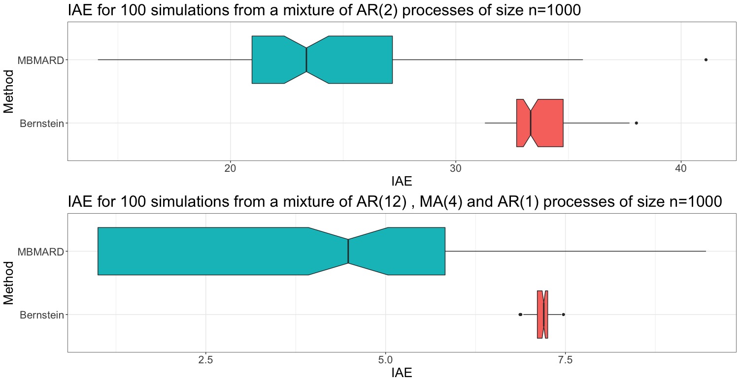
The discrepancy between the estimated and true spectral matrices is computed through the integrated absolute error (IAE) which we define as follows. Let and be the elements of the estimated and true spectral matrices for the observed a multivariate time series respectively. Due to and are hermitian, it is sufficient to compute the error for the lower triangular part of the matrices, then the integrated absolute error is . The MBMARD estimations outperform the estimations based on Bernstein polynomials as shown in Figure 5 boxplots of the IAE for the 100 simulated multivariate signals.
The MBMARD algorithm was run in a HPC cluster formed by Intel Cascade Lakes (40 cores), Skylakes (40 cores), AMD Rome (108 cores) assigned through the workload manager Slurm. The computational performance was, on average, 2 hours and a half for the misspecification scenario and 3 hours and a half for the AR(2) mixture scenario. The Bernstein polynomial method, on average, takes 6 hours to finish 50000 iterations for both scenarios. The difference in computational efficiency is due mainly to the order of updates. MBMARD maintains a small number of kernels by detecting only prominent peaks. At the same time, the Bernstein polynomial relies on increasing the number of kernels to achieve better accuracy in estimating the spectral curves. MBMARD and the Bernstein polynomial method take around 1 hour and a half to run 50000 iterations in both vector autoregressive scenarios.
5 Comparative analysis from EEG of an Alcoholic and a Non-alcoholic subjects
Memory studies are essential to discover the factors affecting memory performance. For instance, there is evidence of long terms affectations of alcoholism on retrieving visual information (see Zhanga et al. 1997; Zhang et al. 1997 ). However, other studies found alcohol consumption effects on memory seem negligible on retrieving information about words (Zhang et al. 1997).
According to Kelley and Lindsay 1996, the brain retrieves better the meaning associated to words than trying to remember their superficial features like shape. Another theory on human memory says that neuronal processes driven by consciously encoding memories, called explicit memory, are affected unconsciously by past experiences or implicit memory(see Schacter et al. 1993). Other studies point to evidence that different populations have different signals behavior when performing implicit or explicit memory tasks (Kelley and Lindsay 1996). Neuroscientists have reached these conclusions by obtaining electroencephalogram (EEG) records as a non-invasive technique to measures electrical signals across the scalp.
The EEG recordings of two subjects, one alcoholic and one non-alcoholic, are analyzed via MBMARD to identify subject-specific dependency within and across brain regions. The MBMARD’s properties to decompose multivariate brain signals in its fundamental latent waves allows the comparison of both subjects. This approach can potentially be extended to infer and compare recording from populations using hierarchical modeling, however, that extension goes beyond the goal of this paper that introduces and demonstrate the advantages of this multivariate methodology.
The experiment consists of presenting to each subject images for 300 ms over three different paradigms. In the first task, a single image is presented to the subject during the 3 seconds trial (Single). In the second task is shown twice the same image (Matching), while in the third task, each subject is exposed to two different images (No Match). The data were recorded at a sample rate of 256 Hz for 1 second for ten trials for each task. See Zhang et al. 1995 for a detailed and technical description of the data acquisition.
The MBMARD method was applied over 61 EEG channels for ten trials running 50,000 iterations for three chains leaving a burn-in period of 30,000 iterations. The estimated location parameters were grouped for all the trials in three of the classic prespecified frequency bands, delta (0-4 Hertz), Theta (4-8 Hertz), Alpha (8-12 Hertz), Beta (12-30 Hertz), Gamma (30-60 Hertz).
The alcoholic subject shows two principal spectral peaks. The first peak is located in the theta band. Figure 6 shows that the theta component is a sharp peak centered around 4-5 Hertz. The Theta peak appears over the frontal and occipital zones in some trials for all the experimental conditions. The Second peak lies on the Gamma band, with higher weights in both temporal zones, but is only found in the Single and No match trials. Contrary to the Theta peak, the Gamma peak is a broad peak with more variability in its centers. Table 1 contains the estimated average parameters of the peaks extracted from the alcoholic subject EEG data for each task.

| Band | Task | (Hz) | # Trials | ||
| Theta | Single | 4.25 | 0.02 | .65 | 3 |
| Match | 4.44 | 0.02 | .68 | 3 | |
| No Match | 4.35 | 0.03 | .67 | 3 | |
| Gamma | Single | 31.7 | 0.32 | .47 | 5 |
| No Match | 32.8 | 0.41 | .48 | 3 |
The Non-alcoholic subject shows a low-frequency component found in the Alpha band for the occipital brain region. This peak has high variability concerning its central location, bandwidth, and weight. Despite being found in several trials, the Alpha component indicates a non-stable behavior of the Alpha oscillations.
The Gamma band contains the second identified peak. However, the Gamma peak is such broad that the latent process estimated includes several oscillations at different frequencies. It is noted that only the peak during a No Match trial is sharp enough to be associated with a quasiperiodic process. The summary of the parameters of the peaks for the Non-alcoholic subject is displayed in Table 2.
The low-frequency components are consistent with the neuroscientific literature since according to DiCarlo et al. 2013 the ventral stream, which is located in the occipital and temporal zone, is where our brain processes object recognition.
Another analysis of the alcoholics and healthy subjects data set has centered on two goals. The first approach is to develop methods that use the EEG recordings or their features as inputs of classification algorithms to predict if a subject is an alcoholic or healthy subject. However, these methods do not delve into the features that help to differentiate between subjects and focus only on accuracy performance (See Palaniappan et al. 2002, Kok-Meng Ong et al. 2005, Yazdani and Kamaledin Setarehdan 2007, Guntaka and Tcheslavski 2013).

| Band | Task | (Hz) | # Trials | ||
|---|---|---|---|---|---|
| Alpha | Single | 10.2 | 0.03 | .34 | 3 |
| Match | 11 | 0.08 | .64 | 6 | |
| No Match | 10.7 | 0.05 | .61 | 5 | |
| Gamma | Single | 30.7 | 0.38 | .47 | 2 |
| Match | 30.6 | 0.6 | .28 | 4 | |
| No Match | 38.7 | 0.05 | .15 | 1 |
The second approach decomposes each channel signal according to frequency bands, analyzing each band’s power and making a comparative analysis. For instance, Sun et al. 2006 uses PCA for dimension reduction and then applies a wavelet decomposition into five frequency bands, finding an increased theta and delta power and a lower power in the alpha band for alcoholics subjects. However, they used different frequency bands, making it difficult to compare with analysis and reinforce the idea or use frequency-specific methods to identify the signals waveforms.
Tcheslavski and Gonen 2012 comprehensively analyzed frequency bands difference in spectral power, coherence, and phase synchrony frequency bands between alcoholics and non-alcoholics, evaluating the significance of the differences using Kruskall-Wallis tests. The authors found that alcoholic’s lower rhythms have lower spectral power and coherence. Delta and Theta rhythms show higher differences in the frontal region, while bands from 8-20 Hz highlight differences in the occipital region.
Our analysis is consistent with previous reports by finding that low-frequency waveforms contribute the highest to the spectral matrix in the frontal and occipital zones. Besides, an additional component was found in the gamma band on the temporal zones. Individual runs of our algorithm to the rest of the subjects in the data set (not shown here) are consistent with our previous findings. However, variability exists across subjects in the peak locations, bandwidths, and weights that should be treated in a hierarchical model.
In brief, the contributions of MBMARD to the alcoholic and healthy subject analysis are 1) the joint modeling of the EEG nodes finding shared information and dependence among the signals, 2) The identification of frequency-specific waveforms in the signals, zooming the analysis into particular frequencies, and making the segmentation by frequency bands optional for comparison with other analysis.
6 Conclusion
The Multivariate Bayesian Mixture Autoregressive Decomposition (MBMARD) is a novel Bayesian non-parametric method that employs the spectral densities of an AR(2) as an unimodal kernel that decompose a multivariate time series into latent stochastic processes.
The parametric kernel allows the straightforward derivation of classical dependence measures as cross-correlation and PDC between the signals in terms of the model parameters, providing a tool to display the association between the channels from the shared latent waveforms.
The Simulations study shows that MBMARD generates a smooth estimator of the spectral density matrix finding the most prominent peak activity of the signals. The computational performance of MBMARD has shown to be more efficient due to maintaining a lower number of components.
The analysis of two subject’s 61 channels EEG dataset via MBMARD highlighted two components in the signals low-frequency and high-frequency oscillations, activated in different zones of the brain. The MBMARD analysis isolated these component’s main characteristics, finding differences in frequency location, shape, variability, and contribution to the EEG variance. MBMARD provides interpretable properties to analyze brain signals under different contexts. In addition, the straightforward understanding of the time series decomposition makes the proposed method applicable to different contexts in time series analysis.
References
- Baccalá and Sameshima (2001) Baccalá, L. A. and K. Sameshima (2001, May). Partial directed coherence: a new concept in neural structure determination. Biological Cybernetics 84(6), 463–474.
- Baldi and Shahbaba (2020) Baldi, P. and B. Shahbaba (2020, July). Bayesian Causality. The American Statistician 74(3), 249–257.
- Brockwell and Davis (1986) Brockwell, P. J. and R. A. Davis (1986). Time Series: Theory and Methods. Berlin, Heidelberg: Springer-Verlag.
- Bruce et al. (2019) Bruce, S. A., C. Y. Tang, M. H. Hall, and R. T. Krafty (2019). Empirical frequency band analysis of nonstationary time series. Journal of the American Statistical Association 0(0), 1–21.
- Buzsáki (2009) Buzsáki, G. (2009, 01). Rhythms of The Brain, pp. xiv, 448 p.
- Choudhuri et al. (2004) Choudhuri, N., S. Ghosal, and A. Roy (2004). Bayesian estimation of the spectral density of a time series. Journal of the American Statistical Association 99(468), 1050–1059.
- Dai and Guo (2004) Dai, M. and W. Guo (2004, September). Multivariate spectral analysis using Cholesky decomposition. Biometrika 91(3), 629–643.
- Depaoli (2020) Depaoli, S. (2020). The Importance of Prior Sensitivity Analysis in Bayesian Statistics: Demonstrations Using an Interactive Shiny App. Frontiers in Psychology 11, 18.
- Deshpande et al. (2009) Deshpande, G., S. LaConte, G. A. James, S. Peltier, and X. Hu (2009). Multivariate Granger causality analysis of fMRI data. Human Brain Mapping 30(4), 1361–1373. _eprint: https://onlinelibrary.wiley.com/doi/pdf/10.1002/hbm.20606.
- DiCarlo et al. (2013) DiCarlo, J. J., D. Zoccolan, and N. C. Rust (2013). How does the brain solve visual object recognition? pp. 36.
- Dickinson et al. (2018) Dickinson, A., C. DiStefano, D. Senturk, and S. S. Jeste (2018). Peak alpha frequency is a neural marker of cognitive function across the autism spectrum. European Journal of Neuroscience 47(6), 643–651.
- Doppelmayr et al. (1998) Doppelmayr, M., W. Klimesch, T. Pachinger, and B. Ripper (1998). Individual differences in brain dynamics: important implications for the calculation of event-related band power. Biological cybernetics 79(1), 49–57.
- Dunson et al. (2008) Dunson, D. B., Y. Xue, and L. Carin (2008, March). The Matrix Stick-Breaking Process. Journal of the American Statistical Association 103(481), 317–327. Publisher: Taylor & Francis _eprint: https://doi.org/10.1198/016214507000001364.
- Eddelbuettel and François (2011) Eddelbuettel, D. and R. François (2011). Rcpp: Seamless R and C++ integration. Journal of Statistical Software 40(8), 1–18.
- Escobar and West (1995) Escobar, M. D. and M. West (1995). Bayesian density estimation and inference using mixtures. Journal of the american statistical association 90(430), 577–588.
- Ferguson (1973) Ferguson, T. S. (1973). A bayesian analysis of some nonparametric problems. The annals of statistics, 209–230.
- Gao et al. (2016) Gao, X., W. Shen, B. Shahbaba, N. Fortin, and H. Ombao (2016). Evolutionary state-space model and its application to time-frequency analysis of local field potentials. arXiv preprint arXiv:1610.07271.
- Geweke (1982) Geweke, J. (1982, June). Measurement of Linear Dependence and Feedback between Multiple Time Series. Journal of the American Statistical Association 77(378), 304–313.
- Grabner et al. (2007) Grabner, R. H., C. Brunner, R. Leeb, C. Neuper, and G. Pfurtscheller (2007). Event-related eeg theta and alpha band oscillatory responses during language translation. Brain research bulletin 72(1), 57–65.
- Granados-Garcia et al. (2021) Granados-Garcia, G., M. Fiecas, S. Babak, N. J. Fortin, and H. Ombao (2021). Brain waves analysis via a non-parametric bayesian mixture of autoregressive kernels. Computational Statistics & Data Analysis, 107409.
- Granger (1963) Granger, C. (1963, March). Economic processes involving feedback. Information and Control 6(1), 28–48.
- Guntaka and Tcheslavski (2013) Guntaka, R. and G. V. Tcheslavski (2013). On the EEG-based Automated Detection of Alcohol Dependence. pp. 10.
- Hart et al. (2022) Hart, B., M. Guindani, S. Malone, and M. Fiecas (2022). A nonparametric Bayesian model for estimating spectral densities of resting-state EEG twin data. Biometrics 78(1), 313–323. _eprint: https://onlinelibrary.wiley.com/doi/pdf/10.1111/biom.13393.
- Hosoya (1991) Hosoya, Y. (1991, December). The decomposition and measurement of the interdependency between second-order stationary processes. Probability Theory and Related Fields 88(4), 429–444.
- Ishwaran and James (2002) Ishwaran, H. and L. F. James (2002). Approximate dirichlet process computing in finite normal mixtures: smoothing and prior information. Journal of Computational and Graphical statistics 11(3), 508–532.
- Jaušovec and Jaušovec (2000) Jaušovec, N. and K. Jaušovec (2000). Differences in event-related and induced brain oscillations in the theta and alpha frequency bands related to human intelligence. Neuroscience letters 293(3), 191–194.
- Kaminski and Blinowska (1991) Kaminski, M. J. and K. J. Blinowska (1991, July). A new method of the description of the information flow in the brain structures. Biological Cybernetics 65(3), 203–210.
- Kelley and Lindsay (1996) Kelley, C. M. and D. S. Lindsay (1996). Chapter 2 - Conscious and Unconscious Forms of Memory. In E. L. Bjork and R. A. Bjork (Eds.), Memory, pp. 31–63. San Diego: Academic Press.
- Klimesch (1997) Klimesch, W. (1997). Eeg-alpha rhythms and memory processes. International Journal of psychophysiology 26(1-3), 319–340.
- Kok-Meng Ong et al. (2005) Kok-Meng Ong, K.-H. Thung, Chong-Yaw Wee, and R. Paramesran (2005). Selection of a Subset of EEG Channels using PCA to classify Alcoholics and Non-alcoholics. In 2005 IEEE Engineering in Medicine and Biology 27th Annual Conference, Shanghai, China, pp. 4195–4198. IEEE.
- Krafty and Collinge (2013) Krafty, R. T. and W. O. Collinge (2013, June). Penalized multivariate Whittle likelihood for power spectrum estimation. Biometrika 100(2), 447–458.
- Krystal et al. (1999) Krystal, A. D., R. Prado, and M. West (1999). New methods of time series analysis of non-stationary eeg data: eigenstructure decompositions of time varying autoregressions. Clinical Neurophysiology 110(12), 2197–2206.
- Li et al. (2020) Li, L., D. Pluta, B. Shahbaba, N. Fortin, H. Ombao, and P. Baldi (2020). Modeling Dynamic Functional Connectivity with Latent Factor Gaussian Processes. pp. 22.
- Lindquist (2008) Lindquist, M. A. (2008, November). The Statistical Analysis of fMRI Data. Statistical Science 23(4).
- Liu et al. (2021) Liu, Y., M. Taniguchi, and H. Ombao (2021, February). Statistical Inference for Local Granger Causality.
- Meier et al. (2019) Meier, A., C. Kirch, M. C. Edwards, and R. Meyer (2019). beyondWhittle: Bayesian Spectral Inference for Stationary Time Series. R package version 1.1.1.
- Meier et al. (2020) Meier, A., C. Kirch, and R. Meyer (2020). Bayesian nonparametric analysis of multivariate time series: A matrix gamma process approach. Journal of Multivariate Analysis 175, 104560.
- Motta and Ombao (2012) Motta, G. and H. Ombao (2012). Evolutionary factor analysis of replicated time series. Biometrics 68(3), 825–836.
- Ombao and Pinto (2021) Ombao, H. and M. Pinto (2021). Spectral dependence. arXiv preprint arXiv:2103.17240.
- Ombao and Van Bellegem (2008) Ombao, H. and S. Van Bellegem (2008). Evolutionary coherence of nonstationary signals. IEEE Transactions on Signal Processing 56(6), 2259–2266.
- Palaniappan et al. (2002) Palaniappan, R., P. Raveendran, and S. Omatu (2002, March). VEP optimal channel selection using genetic algorithm for neural network classification of alcoholics. IEEE Transactions on Neural Networks 13(2), 486–491.
- Petrone (1999) Petrone, S. (1999). Bayesian density estimation using bernstein polynomials. Canadian Journal of Statistics 27(1), 105–126.
- Pinto-Orellana et al. (2021) Pinto-Orellana, M. A., P. Mirtaheri, H. L. Hammer, and H. Ombao (2021). Scau: Modeling spectral causality for multivariate time series with applications to electroencephalograms. arXiv preprint arXiv:2105.06418.
- Prado (1998) Prado, R. (1998). Latent structure in non-stationary time series. Duke University.
- Prado and Huerta (2002) Prado, R. and G. Huerta (2002). Time-varying autoregressions with model order uncertainty. Journal of Time Series Analysis 23(5), 599–618.
- Prado et al. (2001) Prado, R., M. West, and A. D. Krystal (2001). Multichannel electroencephalographic analyses via dynamic regression models with time-varying lag–lead structure. Journal of the Royal Statistical Society: Series C (Applied Statistics) 50(1), 95–109.
- Roebroeck et al. (2005) Roebroeck, A., E. Formisano, and R. Goebel (2005, March). Mapping directed influence over the brain using Granger causality and fMRI. NeuroImage 25(1), 230–242.
- Rosen and Stoffer (2007) Rosen, O. and D. S. Stoffer (2007, February). Automatic estimation of multivariate spectra via smoothing splines. Biometrika 94(2), 335–345.
- Russell (1913) Russell, B. (1913, June). On the Notion of Cause. Proceedings of the Aristotelian Society 13(1), 1–26.
- Schacter et al. (1993) Schacter, D. L., C. Y. P. Chiu, and K. N. Ochsner (1993, March). Implicit Memory: A Selective Review. Annual Review of Neuroscience 16(1), 159–182.
- Scrucca et al. (2016) Scrucca, L., M. Fop, T. B. Murphy, and A. E. Raftery (2016). mclust 5: clustering, classification and density estimation using Gaussian finite mixture models. The R Journal 8(1), 289–317.
- Sethuraman (1994) Sethuraman, J. (1994). A constructive definition of dirichlet priors. Statistica sinica, 639–650.
- Shumway and Stoffer (2017) Shumway, R. H. and D. S. Stoffer (2017). Time series analysis and its applications: with R examples. Springer.
- Sun et al. (2006) Sun, Y., N. Ye, and X. Xu (2006). EEG Analysis of Alcoholics and Controls Based on Feature Extraction. In 2006 8th international Conference on Signal Processing, Guilin, China, pp. 4128837. IEEE.
- Tcheslavski and Gonen (2012) Tcheslavski, G. V. and F. F. Gonen (2012, April). Alcoholism-related alterations in spectrum, coherence, and phase synchrony of topical electroencephalogram. Computers in Biology and Medicine 42(4), 394–401.
- Wei (2019) Wei, W. W. (2019, February). Multivariate spectral analysis of time series. In Multivariate Time Series Analysis and Applications, pp. 301–436. Chichester, UK: John Wiley & Sons, Ltd. Series Title: Wiley Series in Probability and Statistics.
- West (1995) West, M. (1995, December). Bayesian Inference in Cyclical Component Dynamic Linear Models. Journal of the American Statistical Association 90(432), 1301–1312. Publisher: Taylor & Francis _eprint: https://www.tandfonline.com/doi/pdf/10.1080/01621459.1995.10476634.
- West (1997) West, M. (1997). Time series decomposition. Biometrika 84(2), 489–494.
- West et al. (1999) West, M., R. Prado, and A. D. Krystal (1999, June). Evaluation and Comparison of EEG Traces: Latent Structure in Nonstationary Time Series. Journal of the American Statistical Association 94(446), 375–387. Publisher: Taylor & Francis _eprint: https://www.tandfonline.com/doi/pdf/10.1080/01621459.1999.10474128.
- Whittle (1953) Whittle, P. (1953). The Analysis of Multiple Stationary Time Series. Journal of the Royal Statistical Society. Series B (Methodological) 15(1), 125–139. Publisher: [Royal Statistical Society, Wiley].
- Yazdani and Kamaledin Setarehdan (2007) Yazdani, A. and S. Kamaledin Setarehdan (2007, February). Classification of EEG signals correlated with alcohol abusers. In 2007 9th International Symposium on Signal Processing and Its Applications, Sharjah, United Arab Emirates, pp. 1–4. IEEE.
- Zhang et al. (1997) Zhang, X. L., H. Begleiter, and B. Porjesz (1997, October). Do chronic alcoholics have intact implicit memory? An ERP study. Electroencephalography and Clinical Neurophysiology 103(4), 457–473.
- Zhang et al. (1997) Zhang, X. L., H. Begleiter, B. Porjesz, and A. Litke (1997, December). Electrophysiological evidence of memory impairment in alcoholic patients. Biological Psychiatry 42(12), 1157–1171.
- Zhang et al. (1995) Zhang, X. L., H. Begleiter, B. Porjesz, W. Wang, and A. Litke (1995, January). Event related potentials during object recognition tasks. Brain Research Bulletin 38(6), 531–538.
- Zhanga et al. (1997) Zhanga, X.-L., H. Begleitera, and B. Porjesz (1997, September). Is working memory intact in alcoholics? An ERP study. Psychiatry Research: Neuroimaging 75(2), 75–89.
Appendix
The Partial directed coherence of the MBMARD model can be computed explicitly, since the MBMARD model has the same structure as a vector autoregressive model by assuming the signals are a convex combination of the latent oscillations.
The PDC matrix based on the notation of Baccalá and Sameshima 2001 is derived in the following way. First, we define the matrix as the sum of Fourier transform of the coefficient matrices and corresponding to the first and second-order lag, respectively, giving the following block matrix to then compute
The bottom left block from the matrix is the influence of the latent oscillations to the signals expressed as follows,
All the columns have the same factor due to and are diagonal matrices. Denote the common factor per column as for . To standarize the PDC values we denote as the -th column of the matrix then the PDC from the to () is computed as:
where indicate the transpose conjugate. in terms of the parameters the denominator is derived as
where the right term in the sum comes from the diagonal matrix in the upper left block from . The numerator of the PDC is therefore, we can simplify the case when is of interest the PDC from the latent oscillation to the signal in terms of the model parameters through
The other case of interest is the PDC between the signals; however, derived from the identifiability conditions of the model the bottom right side of the block matrix is the identity that leads to the PDC from signal to () be defined as
Therefore, all the associations between the signals are given through their shared latent waves.