Spectral-partitioned Kohn-Sham density functional theory

Consider a many-electron system in an external ionic potential $\hat{V}_{ie}(\{{\bf R}\})$, with the nuclei at positions $\{{\bf R}\}$ in a periodic array of unit cells each containing $N_{at}$ atoms in a volume $\Omega$. Ensemble Kohn-Sham DFT maps this system onto a reference system of non-interacting electrons in an external self-consistent potential $\hat{V}_{KS}$. The state of the non-interacting system is completely described by the ensemble density operator $\hat{\rho}$, whose real-space representation is the density matrix $\rho({\bf r^{\prime}},{\bf r})$ defined as

where the ${\bf k}$-index enumerates $N_{BZ}$ Bloch wave vectors on a uniform grid spanning the first BZ, $n$ enumerates bands, $\psi_{{\bf k}n}({\bf r})$ are the KS wavefunctions, and $f_{{\bf k}n}$ are occupation probabilities required to be non-negative, $f_{{\bf k}n}\geq 0$, and are derived from ensemble statistics, as shown below. The discrete grid of Bloch wave vectors derives from the Born von Karman (BvK) boundary condition on the wavefunctions. Within the BvK supercell, every pair of Bloch wavefunctions with wave vectors ${\bf k}\neq{\bf k^{\prime}}$ are orthogonal. Furthermore, finite systems can be represented with periodic boundary conditions in the limit of vanishing density of ions in each unit cell.

In the following, the domain of all integrals is the unit cell volume $\Omega$ unless otherwise specified. Also, we define the Bloch wavefunctions as

where $u_{{\bf k}n}$ have the periodicity of the lattice and are normalized in the unit cell.

As a result of Bloch’s theorem, the density matrix $\hat{\rho}$ can be decomposed into Bloch-wave components

with the property that every pair of Bloch-wave components $\hat{\rho}_{\bf k}$ and $\hat{\rho}_{\bf k^{\prime}}$ with ${\bf k}\neq{\bf k^{\prime}}$ are orthogonal in the BvK supercell, i.e.,

for all ${\bf r^{\prime}}$ and ${\bf r^{\prime\prime}}$ in the BvK cell. Hence, the KS problem is separable with respect to the lattice-periodic operators ${\hat{\rho}_{\bf k}}$,

which contain all the variational degrees of freedom.

The charge density $n({\bf r})$ is obtained as the diagonal of the DM

The Helmholtz free energy of the non-interacting system in the absence of the self-consistent potential $\hat{V}_{KS}$ can be written

where the non-interacting kinetic energy $T_{s}[\hat{\rho}]$ takes on the form

and the entropy function $S[\hat{\rho}]$ is specified by the ensemble statistics and $\tau_{e}$ is the associated temperature. Note that the $\Tr$ operator in Eq. (7) corresponds to integration over a single unit cell and therefore we have

With the non-interacting free energy $\mathcal{A}_{KS}$ defined, the total ensemble-KS free-energy $F_{KS}$ can be written as a functional of the DM $\hat{\rho}$ at temperature $\tau_{e}$ in an external potential $\hat{V}_{ie}(\{{\bf R}\})$

where

Above, $\hat{V}_{ie}(\{{\bf R}\})$ is the electron-ion interaction potential operator that is allowed to be nonlocal within each atomic sphere in case ions are replaced by pseudopotentials. In Eq. (11), ${\bf T}$ denotes the set of periodic lattice translation vectors, and in Eq. (12), the nuclear positions are expanded as ${\bf R}={\bf T}+{\bf s}_{i}$, where ${\bf s_{i}}$ specify the positions of atoms within each unit cell. In Eq. (10), $F_{xc}[\hat{\rho},\tau_{e}]$ is the contribution of the electronic exchange and correlation (XC) to the free energy, which in general has explicit temperature dependence Karasiev et al. 2014; Karasiev et al. 2018; Groth et al. 2017. Within the most commonly used approximations in KS-DFT Perdew et al. 1996, $F_{xc}$ is a functional of the diagonal elements of the DM only, i.e., charge density $n({\bf r})$ and its gradients, but XC functionals with explicit dependences on off-diagonal elements of the DM, such as hybrid exchange Adamo and Barone 1999; Heyd et al. 2003; Mihaylov et al. 2020 and meta-GGA Sun et al. 2015; Karasiev et al. 2022 are becoming increasingly popular.

The formalism developed in the following is general. However, for the sake of illustration, we will focus on application to warm-dense matter, where a large number of partially occupied orbitals must be accounted for whose occupation probabilities $f_{{\bf k}n}$ are distributed according to Fermi-Dirac (FD) statistics. Below, we derive the associated entropy function $S[\hat{\rho}]=S^{FD}[\hat{\rho}]$. Generalization to other statistical ensembles is straightforward.

Let us start by formulating the expression for the equilibrium ensemble-KS free-energy $\Omega_{KS}$. This can be obtained by constrained minimization of $F_{KS}$ with respect to $\hat{\rho}$, which involves the variational degrees of freedom $\{u_{{\bf k}n}\}$ and $\{f_{{\bf k}n}\}$

Above, the second term on the right-hand side constrains the total number of electrons $N_{e}$, the last term enforces orthonormalization of the KS wavefunctions, and $\mu$ and $\Lambda_{nm}^{\bf k}$ are the associated Lagrange multipliers. It should be noted that within this formulation, no constraints are imposed on the XC potential to be multiplative and local. Hence, for XC functionals that depend explicitly on off-diagonal elements of the DM, such as meta-GGA and hybrid-exchange, the above procedure leads to semi-local or nonlocal XC potentials, which result in self-consistent Hamiltonians that belong to the generalized-KS framework Perdew et al. 2017; Garrick et al. 2020. Inclusion of potential constraints that enforce rigorous KS mapping to fictitious non-interacting systems in a self-consistent optimized effective potential (OEP) Görling 2005 are not considered in the present work. While spectral partitioning can in principle provide a powerful way to simplify the OEP integro-differential equations, the tools developed in this work are not immediately applicable to that problem.

At equilibrium, the KS wavefunctions $\psi_{{\bf k}n}$ become eigenfunctions of the self-consistent Hamiltonian $\hat{H}^{KS}$, which can be obtained through functional differentiation of $E_{KS}$ in Eq. (10) with respect to $\hat{\rho}$ defined in Eq. (1):

where for brevity, we have suppressed the dependence of $E_{KS}$ and $\hat{H}^{KS}$ on $\{{\bf R}\}$ and $\tau_{e}$. The differentiation in Eq. (15), in the BvK supercell, leads to

with $V_{H}({\bf r})=\delta E_{H}/\delta n({\bf r})$, $\bigl<{\bf r^{\prime}}\big|\hat{V}_{ie}[\{{\bf R}\}\big|{\bf r}\bigr>$ defined in Eq. (12), and

where we have explicitly presented the dependences of the various potentials on the temperature $\tau_{e}$, ionic positions $\{{\bf R}\}$, and the DM $\rho^{KS}$. Note that for XC functionals that only depend on the density $n({\bf r})$ and its gradients, the XC potential becomes multiplicative and local: $\bigl<{\bf r^{\prime}}\big|\hat{V}^{xc}[n,\tau_{e}]\big|{\bf r}\bigr>=\delta({\bf r}-{\bf r^{\prime}})\delta F_{xc}[n,\tau_{e}]/\delta n({\bf r})$.

At equilibrium, the Lagrange multiplier matrices $\Lambda_{nm}^{\bf k}$ become diagonal,

where $\hat{H}^{KS}_{\bf k}$ are lattice-periodic Bloch-wave components of the KS Hamiltonian defined as

and can be obtained through functional differentiation of $E_{KS}$ in Eq. (10) with respect to $\hat{\rho}_{\bf k}$ defined in Eq. (5):

Finally, at equilibrium the occupation probabilities become solutions to the equations

where $\mu$ acts as the chemical potential. The left-hand side of the above equation is obtained by partial differentiation of the free energy expression Eq. (10) with respect to occupations $f_{{\bf k}n}$. Within FD statistics, the occupation probabilities are distributed according to

By inserting Eq. (21) into Eq. (22), a relation for the FD entropy function $S^{FD}[\hat{\rho}]$ can be obtained

with $\dot{S}^{FD}(f)=\frac{dS^{FD}}{df}$. Equation (23) can be solved analytically for $\dot{S}^{FD}$, and integrated to obtain the FD entropy function $S^{FD}$ using the boundary condition $S^{FD}(0)=0$, which subsequently can be written as

By inserting the FD occupations Eq. (22) into Eq. (1), and using the diagonal representation of the KS Hamiltonian

the following relation can be derived between the equilibrium DM and the KS Hamiltonian operators

where $\hat{I}$ is the identity operator. Likewise, using the diagonal representation of $\hat{H}^{KS}_{\bf k}$

we can derive the following operator relation

At high electron temperatures the FD distribution becomes broad with a long spectral tail leading to finite occupations at very high energies $\epsilon_{{\bf k}n}$, which in turn makes orbital-based electronic-structure calculations in the regime of warm-dense matter computationally very expensive. One way around this problem has been suggested by Zhang et al. Zhang et al. 2016 to in effect, approximate the KS Hamiltonian at high energies by the HEG one

where $U_{0}^{HEG}$ is a constant potential aligning $\hat{H}^{A}$ with the system’s Hamiltonian $\hat{H}^{KS}$, Eq. (16). In practice, in this scheme a splitting energy is chosen below which the equilibrium DM is spanned by the KS eigenfunctions and above which it is replaced by

Since the computational cost of evaluating $\hat{\rho}^{A}$ is negligible, dramatic savings in computational cost can be achieved if the splitting energy can be pushed down to small values.

Two features of the technique described above need elaboration: (i) how best to join the two DMs $\hat{\rho}^{KS}$ and $\hat{\rho}^{A}$, and (ii), the best choice for the alignment energy $U^{HEG}_{0}$. A number of proposals for solving these problems have been presented in previous publications Zhang et al. 2016; Blanchet et al. 2022a. However, no rigorous framework for an optimal technique has been proposed.

In the following, we derive such a framework. In order to do so, one needs to step back from Eq. (29) and instead build the spDFT formalism from bottom up, starting from a general ansatz for a DM partitioned into two spectral domains: (i) a low-energy subspace spanned by KS eigenstates $\{\psi_{{\bf k}n}\}$, and (ii) a high-energy subspace spanned by another complete set of orthonormal Bloch states $\{\psi^{h}_{{\bf k}n}\}$ that need not be eigenstates of the KS Hamiltonian. We then derive the expression for the free-energy functional whose variational minimium is the optimal DM that is partitioned according to the ansatz given above. Subsequently, in Sec. IV we revisit the problem of electronic structure calculations at extreme temperatures and spectral partitioning with the HEG at high energies. We derive detailed expressions for the spectral-partitioned KS Hamiltonian, forces, and stresses within both PAW and NCPP formalisms.

Before embarking on the derivation of the spDFT functional, we first formulate a template for the spectral partitioned equilibrium DM $\hat{\rho}^{SP}$ that results from variational minimization of this functional. In other words, our aim in this section is to specify our choice of method for joining different DM representations. For this purpose, let us consider the example in the previous subsection, where the KS Hamiltonian at high energies is approximated by $\hat{H}^{A}$ in Eq. (29). Since the Bloch-wave components of the DM are mutually orthogonal, see Eq. (4), they can be spectrally partitioned separately and the splitting energies $\chi_{\bf k}$ are allowed to vary within the BZ. It is however, desirable that the k-dependence of the splitting energies conserve the point group symmetry of the ionic lattice and possibly the time-reversal symmetry to preserve the irreducible wedge in the BZ.

For the following discussion, it suffices to just focus on a single Bloch-wave component $\hat{\rho}^{SP}_{\bf k}$. Preferably, the partition should consist of a smooth interpolation between $\hat{\rho}^{KS}_{\bf k}$ (Eq. (28)) below a splitting energy $\chi_{\bf k}$ and an approximate $\hat{\rho}_{\bf k}^{A}$ (Eq. (30)) above $\chi_{\bf k}$. For this purpose, we employ an analytic partition of unity by a function $\eta(x)$ and its complement $\overline{\eta}(x)=1-\eta(x)$, with $\eta(x)$ being a broadened step function, with $\eta(x)=1$ for $x\rightarrow-\infty$ and $\eta(x)=0$ for $x\rightarrow\infty$. A natural choice is the sigmoid function. As a result, the SP-DM $\hat{\rho}^{SP}_{\bf k}$ becomes

with $\hat{\rho}^{KS}$ and $\hat{\rho}^{A}$ defined in Eqs. 28 and 30 respectively, and

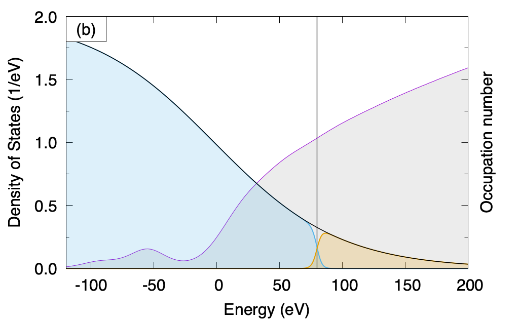
Above, $\eta_{\bf k}(\hat{H}_{\bf k}-\mu\hat{I})$ is the sigmoid function of the Hamiltonian operator relative the chemical potential, centered at the splitting energy $\chi_{\bf k}$, which can be freely chosen for each wave vector ${\bf k}$ separately. The broadening parameter $\tau_{s}$ can also be chosen separately for each wave vector k but it is only a regularization parameter for enhancing numerical stability and therefore we choose to work with a single $\tau_{s}$ value with $\tau_{s}\ll\tau_{e}$. Figure 1 illustrates a typical spectral splitting of the FD distribution as described above.

In the following, we address the central problem of this paper, which is to construct a variational free-energy functional whose equilibrium DM is the SP-DM $\hat{\rho}^{SP}$ in Eq. (31). Subsequently, we derive a general force theorem that facilitates implementation of atomic forces within various electronic structure methodologies.

Consider the Hilbert space spanned by a complete set of orthonormal Bloch wavefunctions $\big|\psi^{h}_{{\bf k}n}\bigr>$ subject to the same BvK boundary condition as the KS wavefunctions $\big|\psi_{{\bf k}n}\bigr>$. Hence, as in Eq. (2), $\psi^{h}_{{\bf k}n}$ can be written in terms of functions $u^{h}_{{\bf k}n}$ with lattice periodicity as

where $u^{h}_{{\bf k}n}({\bf r})$ are normalized within each unit cell. The two Hilbert spaces can be transformed into one another by unitary operators $U_{{\bf k},nm}$

We define the class of Hamiltonians that are diagonal in this basis

where $\epsilon^{h}_{{\bf k}n}$ are real-valued coefficients. Given any parameterization of $\hat{H}^{h}$, we determine the ensemble density operator $\hat{\rho}^{h}$ at temperature $\tau_{e}$ by Eq. (30), which therefore also becomes diagonal in the basis $\big|\psi^{h}_{{\bf k}n}\bigr>$. However, it is important to note that contrary to Eq. (29), we make no assumptions about the coefficients $\epsilon^{h}_{{\bf k}n}$, while at the same time not considering them as variational degrees of freedom.

Our aim is to devise a variational framework whose equilibrium DM can be described by Eq. (31). For this purpose, we decompose each Bloch-wave component of the DM $\hat{\rho}_{\bf k}$ into two contributions $\hat{\rho}^{l}_{\bf k}$ and $\hat{\rho}^{h}_{\bf k}$, with distinct diagonal representations

where $\{Q_{{\bf k}n}\}$, $\{P_{{\bf k}n}\}$, and $\{u_{{\bf k}n}\}$ are variational degrees of freedom. Hence, $\hat{\rho}^{l}_{\bf k}$ are treated fully variationally, while $\hat{\rho}^{h}_{\bf k}$ are only allowed to vary their orbital occupations $P_{{\bf k}n}$. Additionally, the chosen wavefunctions $u^{h}_{{\bf k}n}$ can in principle depend on ion positions. However, for brevity we drop this functional dependence.

In summary, our aim is to construct the spDFT free energy functional in such a way that at its variational minimum, $\rho^{l}$ in Eq. (37) corresponds to the first term on the right-hand side of Eq. (31) and $\rho^{h}$ corresponds to the second. Hence at equilibrium, $\hat{\rho}^{l}$ encompasses the low-energy part of the DM and $\hat{\rho}^{h}$ encompasses the high-energy part.

The Helmholtz free energy of the non-interacting spectral-partitioned system in the absence of the self-consistent potential $\hat{V}_{KS}$ can now be written

with

The non-interacting kinetic energy $T_{s}[\hat{\rho}^{\eta}]$ in Eq. (40) takes on the form

and the spectral-partitioned entropy becomes a functional of the spectral-partitioned DM $\hat{\rho}^{\eta}$, dimensionless ratios of the splitting energies $\chi_{\bf k}$, broadening parameter $\tau_{s}$, and the electron temperature $\tau_{e}$, see Eq. (41). Note that the SP-entropy in Eq. (40) is decomposed into independent contributions from each Bloch-wave component of the SP-DM $\hat{\rho}^{\eta}_{\bf k}$.

Following the steps leading to Eq. (10), we derive the spDFT total free energy functional

where the SP charge density $n^{\eta}$ corresponds to the diagonal elements of the SP-DM $\rho^{\eta}({\bf r},{\bf r})$.

Due to the linearity of the spectral-partitioning ansatz for the DM $\hat{\rho}^{\eta}$ in Eq. (37), functional differentiation of $E_{KS}$ in Eq. (43) with respect to $\hat{\rho}^{\eta}$ recovers the same expression for the spectral-partitioned Hamiltonian as the unpartitioned KS Hamiltonian $\hat{H}^{KS}$ in Eq. (16). Therefore, at equilibrium, the spectral-partitioned energy eigenvalues can be written as

This is an important result. Note that the coefficients $\epsilon^{h}_{{\bf k}n}$ have been completely determined by the variational procedure without ever having been explicitly treated as variational degrees of freedom. In this way, the approximate Hamiltonian $\hat{H}^{h}$ can be determined without any prior assumptions. We see now that the spDFT framework can handle arbitrarily complex approximate Hamiltonians and that the particularly simple form of the HEG Hamiltonian in Eq. (29), with a constant alignment potential $U_{0}^{HEG}$, is an exception, resulting from an intuitive ansatz, rather than the rule. In fact, we will show in section IV.2 that even for the HEG, this is too simple an assumption, and in the presence of NCPP, the HEG Hamiltonian admits a nonlocal potential.

We can now formulate the equilibrium spDFT free energy ${\Omega}_{SP}$, which is obtained by constrained minimization with respect to $\hat{\rho}^{\eta}$ involving the variational degrees of freedom $\{u_{{\bf k}n}\}$, $\{Q_{{\bf k}n}\}$, and $\{P_{{\bf k}n}\}$

At equilibrium, the self-consistent SP-DM $\hat{\rho}^{SP}$ should recover Eq. (31).

The rest of this section will be dedicated to proving the following two theorems.

Theorem I. There exists an electronic entropy function $S^{SP}$ such that at the spDFT equilibrium state corresponding to the variational minimum of the spDFT total free-energy functional in Eq. (43), $\hat{\rho}^{SP}$ recovers the spectral partition of unity in Eq. (31).

Theorem II. The equilibrium spDFT free energy ${\Omega}_{SP}$ is an upper bound to the exact (unpartitioned) KS-DFT free energy, i.e. ${\Omega}_{SP}\left[\{u^{h}\};\{{\bf R}\},\tau_{e},\{\overline{\tau}_{\bf k}\}\right]\geq{\Omega}_{KS}\left[\{{\bf R}\},\tau_{e}\right]$.

Let us start by first proving Theorem I. For this purpose, we construct the entropy function $S^{SP}$, which at the variational minimum that defines $\Omega_{SP}$ in Eq. (46), satisfies the following relations

The energy eigenvalues $\epsilon^{l}_{{\bf k}n}$ and $\epsilon^{h}_{{\bf k}n}$ above are defined in Eqs. (44) and  (45). In order for the equilibrium SP-DM $\hat{\rho}^{SP}$ to satisfy Eq. (31), the solutions of Eqs. (47) and (48) should yield

We start by constructing an entropy function $S^{\eta}(x;\overline{\tau}_{\bf k})$ that can generate Eq. (49) as solution. For brevity, in the following we suppress its parametric dependence and instead denote it by $S^{\eta}_{\bf k}(x)$. Hence, we make the definition

This notation displays the ${\bf k}$-dependence of the splitting energy parameter $\chi_{\bf k}$. We thus insert Eq. (47) into Eq. (49) to obtain

with

Equation (52) must be inverted to obtain $\dot{S}_{\bf k}^{\eta}(x)$. This is possible if $\dot{S}_{\bf k}^{\eta}(x)$ is a monotonic function. But Eq. (52) is a product of two sigmoid functions, each of which are separately invertible and everywhere positive. It is thus easy to see that the product must also be monotonic and thus invertible. This can be rigorously verified by examining the second derivative of the entropy with respect to occupations. For this purpose, we differentiate both sides of Eq. (52) with respect to $x$, and upon rearranging terms, a simple expression for $\ddot{S}_{\bf k}^{\eta}$ can be found:

From the above equation, it can be concluded that $\dot{S}_{\bf k}^{\eta}(x)$ is invertible. In the Appendix, we describe a simple procedure for calculating this function to desired accuracy. Figure 2(a) illustrates $\dot{S}_{\bf k}^{\eta}(x)$ for several choices of the ratios $\tau_{e}/\tau_{s}$ and $\chi_{\bf k}/\tau_{s}$ that are typical for applications to the warm-dense matter regime, presented later in this paper.

It is not as straightforward to construct an entropy function that can generate Eq. (50) as a solution. The reason is that in contrast to Eq. (49), Eq. (50) is not a monotonic function of the entropy derivative defined in Eq. (48). This is also depicted in Fig. 1(b), where the $P_{{\bf k}n}$ distribution defined in Eq. (50) is shown as the envelope of the yellow region. This distribution can instead be obtained as the difference between two monotonic functions: (i) the FD distribution, and (ii) the product of the FD distribution with the cut-off function $\eta_{\bf k}(x)$, shown as the envelope of the blue region in Fig. 1(b). Hence, the high-energy DM $\hat{\rho}^{h}$ can be considered a superposition of fictitious states with positive as well as negative occupations. As a result, the ansatz for $\hat{\rho}^{h}$ in Eq. (39) is incomplete. Rather, it should be broken up into two contributions

where both $P^{+}_{{\bf k}n}$ and $P^{-}_{{\bf k}n}$ need now be treated as independent variational degrees of freedom. Consequently, the total spectral-partitioned entropy function $S^{SP}$ in Eq. (43) takes the form

where $S^{FD}(x)$ is the FD entropy defined in Eq. (24) and the entropy function $S_{\bf k}^{\eta}(x)$ is obtained from Eq. (52). Following the earlier steps in this section, it is straightforward to see that upon minimization, the $Q_{{\bf k}n}$ occupations acquire the distribution in Eq. (49) and the other ones become

Hence, at the variational minimum, the SP charge density can be written as

with

It should be noted that even if $P^{+}_{{\bf k}n}$ and $P^{-}_{{\bf k}n}$ are allowed to vary independently during minimization of the right-hand side of Eq. (46), their difference at the variational minimum is never negative, and the equilibrium SP charge density is always positive definite. The proof of Theorem I is thus complete.

We now proceed with the proof of Theorem II. Before doing so, let us define for the sake of clarity the term “occupied domain”, which we use in the following to denote the spectral region where either one or both of $Q_{{\bf k}n}$ and $P_{{\bf k}n}=P^{+}_{{\bf k}n}-P^{-}_{{\bf k}n}$ are nonzero.

The proof is conducted in three steps: (i) It is shown that the SP free energy $\Omega_{SP}$ in Eq. (46) becomes equal to the exact KS free energy $\Omega_{KS}$ in Eq. (14), whenever in the occupied domain, the basis functions spanning the high-energy subspace coincide with those spanning the low-energy one, $u^{h}_{{\bf k}n}=u_{{\bf k}n}$. (ii) Under this condition, we prove that the SP free energy is at a local minimum with respect to infinitesimal unitary transformations of $\{u^{h}_{{\bf k}n}\}$. (iii) We show that whenever in the occupied domain, there are basis functions such that $\left<u^{h}_{{\bf k}n}|u_{{\bf k}m}\right>\neq\delta_{nm}$, the SP free energy $\Omega_{SP}$ can be lowered by a unitary transformation of $\{u^{h}_{{\bf k}n}\}$.

We start by proving (i). For this purpose, consider the SP free energy $\Omega_{SP}[\{u_{{\bf k}n}\}]$, where for brevity we have suppressed the dependence on the variables $\{{\bf R}\},\tau_{e},\{\overline{\tau}_{\bf k}\}$. All arguments put forth below should hold for any reasonable choice of these variables. Let us now define the basis functions $w_{{\bf k}n}=u_{{\bf k}n}$ in the occupied domain. We need to show that the following relation holds

where $\Omega_{KS}$ is the exact KS free energy in Eq. (14). This is true because $w_{{\bf k}n}$ are eigenfunctions of the KS Hamiltonian $\hat{H}_{\bf k}^{KS}$ in Eq. (20), and therefore $\epsilon^{h}_{{\bf k}n}=\epsilon^{l}_{{\bf k}n}$ as can be concluded from Eqs. (44) and (45). Consequently, the occupations $P_{{\bf k}n}^{-}=Q_{{\bf k}n}$, see Eqs. (49) and (60), and thus the non-Fermi-Dirac contributions to the entropy function in Eq. (58) cancel and the free energy function ${\Omega}_{KS}$ is recovered. This concludes the proof of (i).

Next we prove (ii). For this purpose, we investigate the variations of ${\Omega}_{SP}$ with respect to the basis functions $u^{h}_{{\bf k}n}$ spanning the high-energy subspace. This is simplified because $\Omega_{SP}$ is already at a variational minimum with respect to the KS orbitals $u_{{\bf k}n}$ as well as the occupations $P^{\pm}_{{\bf k}n}$ and $Q_{{\bf k}n}$. Consequently, the Hellmann-Feynman theorem holds and only partial derivatives of the right-hand side of Eq. (46) with respect to $u^{h}_{{\bf k}n}$ contribute to the functional derivatives of ${\Omega}_{SP}$ leading to

References

- Hamann et al. (1979) D. R. Hamann, M. Schlüter, and C. Chiang, “Norm-conserving pseudopotentials,” Phys. Rev. Lett. 43, 1494–1497 (1979).
- Ihm et al. (1979) J Ihm, A Zunger, and M L Cohen, “Momentum-space formalism for the total energy of solids,” Journal of Physics C: Solid State Physics 12, 4409–4422 (1979).
- Payne et al. (1992) M. C. Payne, M. P. Teter, D. C. Allan, T. A. Arias, and J. D. Joannopoulos, “Iterative minimization techniques for ab initio total-energy calculations: molecular dynamics and conjugate gradients,” Rev. Mod. Phys. 64, 1045–1097 (1992).
- Vanderbilt (1990) David Vanderbilt, “Soft self-consistent pseudopotentials in a generalized eigenvalue formalism,” Phys. Rev. B 41, 7892–7895 (1990).
- Yang (1991) Weitao Yang, “Direct calculation of electron density in density-functional theory,” Phys. Rev. Lett. 66, 1438–1441 (1991).
- Wang et al. (2008) Lin-Wang Wang, Zhengji Zhao, and Juan Meza, “Linear-scaling three-dimensional fragment method for large-scale electronic structure calculations,” Phys. Rev. B 77, 165113 (2008).
- Soven (1967) Paul Soven, “Coherent-potential model of substitutional disordered alloys,” Phys. Rev. 156, 809–813 (1967).
- Aryasetiawan et al. (2009) F. Aryasetiawan, J. M. Tomczak, T. Miyake, and R. Sakuma, “Downfolded self-energy of many-electron systems,” Phys. Rev. Lett. 102, 176402 (2009).
- Georges et al. (1996) Antoine Georges, Gabriel Kotliar, Werner Krauth, and Marcelo J. Rozenberg, “Dynamical mean-field theory of strongly correlated fermion systems and the limit of infinite dimensions,” Rev. Mod. Phys. 68, 13–125 (1996).
- Andersen (1975) O. Krogh Andersen, “Linear methods in band theory,” Phys. Rev. B 12, 3060–3083 (1975).
- Wimmer et al. (1981) E. Wimmer, H. Krakauer, M. Weinert, and A. J. Freeman, “Full-potential self-consistent linearized-augmented-plane-wave method for calculating the electronic structure of molecules and surfaces: molecule,” Phys. Rev. B 24, 864–875 (1981).
- Phillips (1958) James C. Phillips, “Energy-band interpolation scheme based on a pseudopotential,” Phys. Rev. 112, 685–695 (1958).
- Hamann (2013) D. R. Hamann, “Optimized norm-conserving vanderbilt pseudopotentials,” Phys. Rev. B 88, 085117 (2013).
- Blöchl (1994) P. E. Blöchl, “Projector augmented-wave method,” Phys. Rev. B 50, 17953–17979 (1994).
- Zylstra et al. (2022) A. B. Zylstra, O. A. Hurricane, D. A. Callahan, A. L. Kritcher, J. E. Ralph, H. F. Robey, J. S. Ross, C. V. Young, K. L. Baker, D. T. Casey, T. Döppner, L. Divol, M. Hohenberger, S. Le Pape, A. Pak, P. K. Patel, R. Tommasini, S. J. Ali, P. A. Amendt, L. J. Atherton, B. Bachmann, D. Bailey, L. R. Benedetti, L. Berzak Hopkins, R. Betti, S. D. Bhandarkar, J. Biener, R. M. Bionta, N. W. Birge, E. J. Bond, D. K. Bradley, T. Braun, T. M. Briggs, M. W. Bruhn, P. M. Celliers, B. Chang, T. Chapman, H. Chen, C. Choate, A. R. Christopherson, D. S. Clark, J. W. Crippen, E. L. Dewald, T. R. Dittrich, M. J. Edwards, W. A. Farmer, J. E. Field, D. Fittinghoff, J. Frenje, J. Gaffney, M. Gatu Johnson, S. H. Glenzer, G. P. Grim, S. Haan, K. D. Hahn, G. N. Hall, B. A. Hammel, J. Harte, E. Hartouni, J. E. Heebner, V. J. Hernandez, H. Herrmann, M. C. Herrmann, D. E. Hinkel, D. D. Ho, J. P. Holder, W. W. Hsing, H. Huang, K. D. Humbird, N. Izumi, L. C. Jarrott, J. Jeet, O. Jones, G. D. Kerbel, S. M. Kerr, S. F. Khan, J. Kilkenny, Y. Kim, H. Geppert Kleinrath, V. Geppert Kleinrath, C. Kong, J. M. Koning, J. J. Kroll, M. K. G. Kruse, B. Kustowski, O. L. Landen, S. Langer, D. Larson, N. C. Lemos, J. D. Lindl, T. Ma, M. J. MacDonald, B. J. MacGowan, A. J. Mackinnon, S. A. MacLaren, A. G. MacPhee, M. M. Marinak, D. A. Mariscal, E. V. Marley, L. Masse, K. Meaney, N. B. Meezan, P. A. Michel, M. Millot, J. L. Milovich, J. D. Moody, A. S. Moore, J. W. Morton, T. Murphy, K. Newman, J. M. G. Di Nicola, A. Nikroo, R. Nora, M. V. Patel, L. J. Pelz, J. L. Peterson, Y. Ping, B. B. Pollock, M. Ratledge, N. G. Rice, H. Rinderknecht, M. Rosen, M. S. Rubery, J. D. Salmonson, J. Sater, S. Schiaffino, D. J. Schlossberg, M. B. Schneider, C. R. Schroeder, H. A. Scott, S. M. Sepke, K. Sequoia, M. W. Sherlock, S. Shin, V. A. Smalyuk, B. K. Spears, P. T. Springer, M. Stadermann, S. Stoupin, D. J. Strozzi, L. J. Suter, C. A. Thomas, R. P. J. Town, E. R. Tubman, C. Trosseille, P. L. Volegov, C. R. Weber, K. Widmann, C. Wild, C. H. Wilde, B. M. Van Wonterghem, D. T. Woods, B. N. Woodworth, M. Yamaguchi, S. T. Yang, and G. B. Zimmerman, “Burning plasma achieved in inertial fusion,” Nature 601, 542–548 (2022).
- Remington et al. (2006) Bruce A. Remington, R. Paul Drake, and Dmitri D. Ryutov, “Experimental astrophysics with high power lasers and pinches,” Rev. Mod. Phys. 78, 755–807 (2006).
- Lindl et al. (2004) John D. Lindl, Peter Amendt, Richard L. Berger, S. Gail Glendinning, Siegfried H. Glenzer, Steven W. Haan, Robert L. Kauffman, Otto L. Landen, and Laurence J. Suter, “The physics basis for ignition using indirect-drive targets on the national ignition facility,” Physics of Plasmas 11, 339–491 (2004).
- Bostedt et al. (2016) Christoph Bostedt, Sébastien Boutet, David M. Fritz, Zhirong Huang, Hae Ja Lee, Henrik T. Lemke, Aymeric Robert, William F. Schlotter, Joshua J. Turner, and Garth J. Williams, “Linac coherent light source: The first five years,” Rev. Mod. Phys. 88, 015007 (2016).
- Craxton et al. (2015) R. S. Craxton, K. S. Anderson, T. R. Boehly, V. N. Goncharov, D. R. Harding, J. P. Knauer, R. L. McCrory, P. W. McKenty, D. D. Meyerhofer, J. F. Myatt, A. J. Schmitt, J. D. Sethian, R. W. Short, S. Skupsky, W. Theobald, W. L. Kruer, K. Tanaka, R. Betti, T. J. B. Collins, J. A. Delettrez, S. X. Hu, J. A. Marozas, A. V. Maximov, D. T. Michel, P. B. Radha, S. P. Regan, T. C. Sangster, W. Seka, A. A. Solodov, J. M. Soures, C. Stoeckl, and J. D. Zuegel, “Direct-drive inertial confinement fusion: A review,” Physics of Plasmas 22, 110501 (2015).
- Guillot (1999) Tristan Guillot, “Interiors of giant planets inside and outside the solar system,” Science 286, 72–77 (1999).
- Surh et al. (2001) Michael P. Surh, T. W. Barbee, and L. H. Yang, “First principles molecular dynamics of dense plasmas,” Phys. Rev. Lett. 86, 5958–5961 (2001).
- Nagy (2019) A. Nagy, “A thermal orbital-free density functional approach,” The Journal of Chemical Physics 151, 014103 (2019).
- Kang et al. (2020) Dongdong Kang, Kai Luo, Keith Runge, and S. B. Trickey, “Two-temperature warm dense hydrogen as a test of quantum protons driven by orbital-free density functional theory electronic forces,” Matter and Radiation at Extremes 5 (2020), 10.1063/5.0025164.
- Luo et al. (2020) K. Luo, V. V. Karasiev, and S. B. Trickey, “Towards accurate orbital-free simulations: A generalized gradient approximation for the noninteracting free energy density functional,” Phys. Rev. B 101, 075116 (2020).
- Suryanarayana et al. (2018) Phanish Suryanarayana, Phanisri P. Pratapa, Abhiraj Sharma, and John E. Pask, “SQDFT: spectral quadrature method for large-scale parallel o(n) kohn-sham calculations at high temperature,” Computer Physics Communications 224, 288–298 (2018).
- Cytter et al. (2018) Yael Cytter, Eran Rabani, Daniel Neuhauser, and Roi Baer, “Stochastic density functional theory at finite temperatures,” Phys. Rev. B 97, 115207 (2018).
- White and Collins (2020) A. J. White and L. A. Collins, “Fast and universal kohn-sham density functional theory algorithm for warm dense matter to hot dense plasma,” Phys. Rev. Lett. 125, 055002 (2020).
- Starrett and Shaffer (2020) C. E. Starrett and N. Shaffer, “Multiple scattering theory for dense plasmas,” Phys. Rev. E 102, 043211 (2020).
- Driver and Militzer (2012) K. P. Driver and B. Militzer, “All-electron path integral monte carlo simulations of warm dense matter: Application to water and carbon plasmas,” Phys. Rev. Lett. 108, 115502 (2012).
- Driver et al. (2017) K.P. Driver, Francois Soubiran, Shuai Zhang, and B. Militzer, “Comparison of path integral monte carlo simulations of helium, carbon, nitrogen, oxygen, water, neon, and silicon plasmas,” High Energy Density Physics 23, 81–89 (2017).
- Starrett et al. (2015) C. E. Starrett, J. Daligault, and D. Saumon, “Pseudoatom molecular dynamics,” Phys. Rev. E 91, 013104 (2015).
- Starrett and Saumon (2016) C. E. Starrett and D. Saumon, “Equation of state of dense plasmas with pseudoatom molecular dynamics,” Phys. Rev. E 93, 063206 (2016).
- Zhang et al. (2016) Shen Zhang, Hongwei Wang, Wei Kang, Ping Zhang, and X. T. He, “Extended application of Kohn-Sham first-principles molecular dynamics method with plane wave approximation at high energy – From cold materials to hot dense plasmas,” Physics of Plasmas 23, 042707 (2016), https://doi.org/10.1063/1.4947212 .
- Blanchet et al. (2022a) Augustin Blanchet, Francois Soubiran, Marc Torrent, and Jean Clerouin, “Extended first-principles molecular dynamics simulations of hot dense boron: equation of state and ionization,” Contributions to Plasma Physics 62, e202100234 (2022a).
- Blanchet et al. (2020) A. Blanchet, M. Torrent, and J. Clerouin, “Requirements for very high temperature Kohn-Sham DFT simulations and how to bypass them,” Physics of Plasmas 27, 122706 (2020).
- Blanchet et al. (2022b) A. Blanchet, J. Clerouin, M. Torrent, and F. Soubiran, “Extended first-principles molecular dynamics model for high temperature simulations in the abinit code: Application to warm dense aluminum,” Computer Physics Communications 271, 108215 (2022b).
- Hollebon and Sjostrom (2022) P. Hollebon and T. Sjostrom, “Hybrid scheme for high-temperature density functional theory,” Phys. Rev. B 105, 235114 (2022).
- Liu et al. (2021) Xing Liu, Xiaohan Zhang, Chang Gao, Shen Zhang, Cong Wang, Dafang Li, Ping Zhang, Wei Kang, Weiyan Zhang, and X. T. He, “Equations of state of poly--methylstyrene and polystyrene: First-principles calculations versus precision measurements,” Phys. Rev. B 103, 174111 (2021).
- Mermin (1965) N. David Mermin, “Thermal properties of the inhomogeneous electron gas,” Phys. Rev. 137, A1441–A1443 (1965).
- Karasiev et al. (2014) Valentin V. Karasiev, Travis Sjostrom, James Dufty, and S. B. Trickey, “Accurate homogeneous electron gas exchange-correlation free energy for local spin-density calculations,” Phys. Rev. Lett. 112, 076403 (2014).
- Karasiev et al. (2018) Valentin V. Karasiev, James W. Dufty, and S. B. Trickey, “Nonempirical semilocal free-energy density functional for matter under extreme conditions,” Phys. Rev. Lett. 120, 076401 (2018).
- Groth et al. (2017) Simon Groth, Tobias Dornheim, Travis Sjostrom, Fionn D. Malone, W. M. C. Foulkes, and Michael Bonitz, “Ab initio exchange-correlation free energy of the uniform electron gas at warm dense matter conditions,” Phys. Rev. Lett. 119, 135001 (2017).
- Ho et al. (1982) K. M. Ho, C. L. Fu, B. N. Harmon, W. Weber, and D. R. Hamann, “Vibrational frequencies and structural properties of transition metals via total-energy calculations,” Phys. Rev. Lett. 49, 673–676 (1982).
- Methfessel and Paxton (1989) M. Methfessel and A. T. Paxton, “High-precision sampling for brillouin-zone integration in metals,” Phys. Rev. B 40, 3616–3621 (1989).
- Pederson and Jackson (1991) Mark R. Pederson and Koblar A. Jackson, “Pseudoenergies for simulations on metallic systems,” Phys. Rev. B 43, 7312–7315 (1991).
- Wentzcovitch et al. (1992) Renata M. Wentzcovitch, José Luís Martins, and Philip B. Allen, “Energy versus free-energy conservation in first-principles molecular dynamics,” Phys. Rev. B 45, 11372–11374 (1992).
- Weinert and Davenport (1992) M. Weinert and J. W. Davenport, “Fractional occupations and density-functional energies and forces,” Phys. Rev. B 45, 13709–13712 (1992).
- Marzari et al. (1997) Nicola Marzari, David Vanderbilt, and M. C. Payne, “Ensemble density-functional theory for ab initio molecular dynamics of metals and finite-temperature insulators,” Phys. Rev. Lett. 79, 1337–1340 (1997).
- dos Santos and Marzari (2023) Flaviano José dos Santos and Nicola Marzari, “Fermi energy determination for advanced smearing techniques,” Phys. Rev. B 107, 195122 (2023).
- de Gironcoli et al. (1989) Stefano de Gironcoli, Stefano Baroni, and Raffaele Resta, “Piezoelectric properties of iii-v semiconductors from first-principles linear-response theory,” Phys. Rev. Lett. 62, 2853–2856 (1989).
- de Gironcoli (1995) Stefano de Gironcoli, “Lattice dynamics of metals from density-functional perturbation theory,” Phys. Rev. B 51, 6773–6776 (1995).
- Gonze and Vigneron (1989) X. Gonze and J.-P. Vigneron, “Density-functional approach to nonlinear-response coefficients of solids,” Phys. Rev. B 39, 13120–13128 (1989).
- Perdew et al. (1996) John P. Perdew, Kieron Burke, and Matthias Ernzerhof, “Generalized gradient approximation made simple,” Phys. Rev. Lett. 77, 3865–3868 (1996).
- Sun et al. (2015) Jianwei Sun, Adrienn Ruzsinszky, and John P. Perdew, “Strongly constrained and appropriately normed semilocal density functional,” Phys. Rev. Lett. 115, 036402 (2015).
- Anisimov et al. (1997) Vladimir I Anisimov, F Aryasetiawan, and A I Lichtenstein, “First-principles calculations of the electronic structure and spectra of strongly correlated systems: the LDA+U method,” Journal of Physics: Condensed Matter 9, 767 (1997).
- Cococcioni and de Gironcoli (2005) Matteo Cococcioni and Stefano de Gironcoli, “Linear response approach to the calculation of the effective interaction parameters in the method,” Phys. Rev. B 71, 035105 (2005).
- Becke (1993) Axel D. Becke, “A new mixing of Hartree-Fock and local density-functional theories,” J. Chem. Phys. 98, 1372–1377 (1993).
- Adamo and Barone (1999) Carlo Adamo and Vincenzo Barone, “Toward reliable density functional methods without adjustable parameters: The PBE0 model,” The Journal of Chemical Physics 110, 6158–6170 (1999).
- Heyd et al. (2003) Jochen Heyd, Gustavo E. Scuseria, and Matthias Ernzerhof, “Hybrid functionals based on a screened Coulomb potential,” J. Chem. Phys. 118, 8207–8215 (2003).
- Zhao and Truhlar (2006) Yan Zhao and Donald G. Truhlar, “Density Functional for Spectroscopy: No Long-Range Self-Interaction Error, Good Performance for Rydberg and Charge-Transfer States, and Better Performance on Average than B3LYP for Ground States,” Journal of Physical Chemistry A 110, 13126–13130 (2006).
- Mihaylov et al. (2020) D. I. Mihaylov, V. V. Karasiev, and S. X. Hu, “Thermal hybrid exchange-correlation density functional for improving the description of warm dense matter,” Phys. Rev. B 101, 245141 (2020).
- Karasiev et al. (2022) Valentin V. Karasiev, D. I. Mihaylov, and S. X. Hu, “Meta-gga exchange-correlation free energy density functional to increase the accuracy of warm dense matter simulations,” Phys. Rev. B 105, L081109 (2022).
- Perdew et al. (2017) John P. Perdew, Weitao Yang, Kieron Burke, Zenghui Yang, Eberhard K. U. Gross, Matthias Scheffler, Gustavo E. Scuseria, Thomas M. Henderson, Igor Ying Zhang, Adrienn Ruzsinszky, Haowei Peng, Jianwei Sun, Egor Trushin, and Andreas Görling, “Understanding band gaps of solids in generalized Kohn-Sham theory,” Proceedings of the National Academy of Sciences 114, 2801–2806 (2017).
- Garrick et al. (2020) Rachel Garrick, Amir Natan, Tim Gould, and Leeor Kronik, “Exact generalized kohn-sham theory for hybrid functionals,” Phys. Rev. X 10, 021040 (2020).
- Görling (2005) Andreas Görling, “Orbital- and state-dependent functionals in density-functional theory,” The Journal of Chemical Physics 123, 062203 (2005).
- Gillan (1989) M J Gillan, “Calculation of the vacancy formation energy in aluminium,” Journal of Physics: Condensed Matter 1, 689 (1989).
- Kresse and Furthmüller (1996) G. Kresse and J. Furthmüller, “Efficient iterative schemes for ab initio total-energy calculations using a plane-wave basis set,” Phys. Rev. B 54, 11169–11186 (1996).
- Goedecker and Maschke (1992) S. Goedecker and K. Maschke, “Operator approach in the linearized augmented-plane-wave method: Efficient electronic-structure calculations including forces,” Phys. Rev. B 45, 1597–1604 (1992).
- Kresse and Joubert (1999) G. Kresse and D. Joubert, “From ultrasoft pseudopotentials to the projector augmented-wave method,” Phys. Rev. B 59, 1758–1775 (1999).
- Nielsen and Martin (1985a) O. H. Nielsen and Richard M. Martin, “Stresses in semiconductors: Ab initio calculations on si, ge, and gaas,” Phys. Rev. B 32, 3792–3805 (1985a).
- Nielsen and Martin (1985b) O. H. Nielsen and Richard M. Martin, “Quantum-mechanical theory of stress and force,” Phys. Rev. B 32, 3780–3791 (1985b).
- Kleinman and Bylander (1982) Leonard Kleinman and D. M. Bylander, “Efficacious form for model pseudopotentials,” Phys. Rev. Lett. 48, 1425–1428 (1982).
- Klimeš et al. (2014) Jiř’i Klimeš, Merzuk Kaltak, and Georg Kresse, “Predictive gw calculations using plane waves and pseudopotentials,” Phys. Rev. B 90, 075125 (2014).