A graph convolutional autoencoder approach to model order reduction for parametrized PDEs

In recent years, Graph Neural Networks [90, 40] have been an active area of research with rapid growth. GNNs are a specific kind of deep learning architectures capable of extracting information from a graph-structured dataset, including geometric configurations, relationships between nodes and connectivity, and features’ behavior. They are used in different fields such as recommendation systems, social networks and to express molecular structures, for their ability to process non-euclidean data. Several tasks can be performed through GNNs

• $\circ$

  at graph-level: where the goal is the property/label for the whole structure,

• $\circ$

  at node-level: to infer the features at some specific location,

• $\circ$

  at edge-level: to predict the existence of a given link/connection.

The information is usually propagated between nodes through two of the basic operations of GNNs: aggregation and message passing.

A key property of GNNs is that they preserve discrete symmetries, i.e. nodes do not have to be in any specific order when they are provided as input to the network. Consequently, the functions are permutation-invariant. This is a great advantage that allows generalizing common architectures such as Convolutional Neural Networks that require a fixed template/filter. Graph networks have been widely employed in recent research [86]. Notably, it has been especially successful in large deformation settings and complex simulations, drug discovery, and in general in scenarios where data is unstructured.

Focusing on our area of interest, graphs have been applied to the study of computational mechanics for the reconstruction of solution fields [88], the integration of complex systems in time [76], and combined with learning biases to preserve fundamental physical laws [43].

In the model order reduction context, we can discern between two classes. On the one hand, we find those that reduce the mesh to alleviate graph operations [27], and its edge-augmented version [34]. The work by Han et al. [41] fall into first class and focus on preserving the graph information by finding a coarser representation by collapsing nodes to speed up the simulation.

On the other hand, the second class of reduction methods is related to the classical ROM setting, with which a vector low-dimensional representation of the data is found. For example, in [84] the main goal is to deal with 3D representations for reconstruction and tracking. Graph U-nets [32] present an architecture of graph convolutions combined with down-sampling layers that lead to a low dimensional manifold. Ranjan et al. [72] introduce the so-called COMA network consisting of a combination of spectral Chebyshev convolutions [19] and down-sampling operations to generate new faces. In [91], the authors define the pooling operations based on varying kernels formulated at the mesh points. Also, the work of Kashefi et al. [47] presents the reconstruction of solution fields for a given geometry. In the context of parametrized PDEs, we acknowledge the recent work of Gruber et al. [37], which compared different ML approaches for data-driven ROMs, considering spectral convolutions without exploiting down-sampling procedures.

Indeed, the definition of down-sampling and up-sampling operations to coarsen and reconstruct domains is one of the most critical steps for an autoencoder-based architecture. These methods are widely studied for classification problems [13]. However, pooling, un-pooling, and inverse convolutions are not defined for non-euclidean domains. Although there are functions that perform an approximation of these operations [70], their application is still ongoing research. Currently, the most widely used reconstruction function for up-sampling is the one exploiting $k$-nearest neighbors [69]. Finally, we remark that since GNNs are still in their early stage of development, they offer much room for further investigations and developments.

In the field of computational mechanics, the numerical approximation of physical models described by PDEs is of utmost importance. Such models are usually characterized by the domain in which they are posed, geometric and/or physical parameters, and possibly nonlinear terms. The so-called high-fidelity techniques, such as the Finite Element method, involve a large number of degrees of freedom, preventing a fast resolution of the model under investigation. This issue is especially harmful in the parametrized context, when one is interested in recovering the solution for different physical/geometrical configurations, for many-query or real time investigations.

Reduced Order Models have been developed during the last decade to address this computational bottleneck. In particular, the Reduced Basis (RB) method [45, 71] aims at constructing a low-dimensional space which captures the key features of the system. This way, one uses a Galerkin projection to project the model w.r.t. the basis spanning the low-dimensional manifold, to obtain a reduced system.

Given a suitable Hilbert space $\mathbb{X}_{{\boldsymbol{\mu}}}\doteq\mathbb{X}(\Omega({\boldsymbol{\mu}}))$, we consider the nonlinear, steady, and parametrized problem: given $\boldsymbol{\mu}\in\mathcal{P}\subset\mathbb{R}^{P}$, seek $u({\boldsymbol{\mu}})\in\mathbb{X}_{{\boldsymbol{\mu}}}$ such that

where $\boldsymbol{\mu}\in\mathcal{P}$ is the parameter, $\Omega({\boldsymbol{\mu}})$ the computational domain (possibly ${\boldsymbol{\mu}}$-dependent), and $F$ expresses the PDE operator. A possible high-fidelity approach consists in a Galerkin projection of the associated weak-formulation over some finite dimensional subspace $\mathbb{X}_{{\boldsymbol{\mu}}}^{\mathcal{N}}\subset\mathbb{X}_{{\boldsymbol{\mu}}}$ of dimension $\mathcal{N}$.

Thanks to the Newton-Kantorovich method [16], the formulation of the linearized system at the $k$-th iteration reads: given ${\boldsymbol{\mu}}\in\mathcal{P}$, seek $\delta\textbf{u}_{\mathcal{N}}\in\mathbb{R}^{\mathcal{N}}$ such that

where $\mathsf{F}_{\mathcal{N}}\in{\mathbb{R}}^{\mathcal{N}}$ and $\mathsf{J}_{\mathcal{N}}\in{\mathbb{R}}^{{\mathcal{N}}\times{\mathcal{N}}}$ are the high-fidelity residual vector and the Jacobian matrix, respectively. Finally, we update the iteration as $\textbf{u}_{\mathcal{N}}^{k}=\textbf{u}_{\mathcal{N}}^{k-1}+\delta\textbf{u}_{\mathcal{N}}$ until convergence.

Exploiting the same concept in the ROM context, one builds a basis $\{\boldsymbol{\zeta}_{k}\}_{k=1}^{N}\subset\mathbb{X}_{{\boldsymbol{\mu}}}^{\mathcal{N}}$ for the reduced space $\mathbb{X}_{{\boldsymbol{\mu}}}^{N}$, e.g. by means of the POD technique [83], to project the system once again, obtaining the following formulation: given ${\boldsymbol{\mu}}\in\mathcal{P}$, seek $\delta\textbf{u}_{N}\in\mathbb{R}^{N}$ such that

where the basis matrix is encoded in $\mathsf{V}=[\boldsymbol{\zeta}_{1}|\dots|\boldsymbol{\zeta}_{N}]\in\mathbb{R}^{{\mathcal{N}}\times N}$, and we update the iteration as $\textbf{u}_{N}^{k}=\textbf{u}_{N}^{k-1}+\delta\textbf{u}_{N}$. The reduced basis approximation is finally given by, $u_{N}({\boldsymbol{\mu}})=\sum_{k=1}^{N}u_{N}^{(k)}({\boldsymbol{\mu}})\boldsymbol{\zeta}_{k}$, where $\textbf{u}_{N}({\boldsymbol{\mu}})=\{u_{N}^{(k)}({\boldsymbol{\mu}})\}_{k=1}^{N}$ is the reduced coefficient vector.

The POD basis can be extracted by exploiting the FE data, i.e. a set of solutions corresponding to different parameters $\{{\boldsymbol{\mu}}^{i}\}_{i=1}^{N_{\text{S}}}$, the so-called snapshots $\{u_{\mathcal{N}}({\boldsymbol{\mu}}^{i})\}_{i=1}^{N_{\text{S}}}$. The efficiency of the classical approach relies on the affine decomposition assumption, and on the independence of the online computations from the degrees of freedom ${\mathcal{N}}$. Unfortunately, these assumptions are not fulfilled in the general nonlinear context, since (2) requires repeated assembly of the system involving the basis matrix $\mathsf{V}$, drastically compromising the performance. The Empirical Interpolation Method and its variants [4, 14] are affine-recovery techniques which interpolate the non-affine or nonlinear terms, suggesting a considerable speed-up. Such methodologies entail an intrusive approach, requiring the a priori knowledge of the physics and its high-fidelity operators.

As detailed above, the intrusive nature of projection-based model order reduction can jeopardize the goal of traditional reduced order models, i.e. high computational efficiency. Non-intrusive and data-driven ROMs arise as an alternative to these techniques, with the scope of reducing the computational complexity without the need to project the governing equation. The starting point to build such ROMs is the dataset constituted by the aforementioned snapshots. Several linear and nonlinear methodologies have been developed and analyzed, occasionally benefiting by machine learning approaches.

The key reference of the first class is represented by the RB method, expressing the reduced approximation as the linear expansion over the basis functions as $u_{{\mathcal{N}}}({\boldsymbol{\mu}})\approx u_{N}({\boldsymbol{\mu}})=\mathsf{V}\textbf{u}_{N}({\boldsymbol{\mu}})$. While traditional methods require the solution of a reduced (nonlinear) system to obtain the reduced coefficient vector $\textbf{u}_{N}({\boldsymbol{\mu}})$, non-intrusive approaches exploit different workarounds to replace this step.

Proper Orthogonal Decomposition with interpolation (PODI) [12, 20] projects the snapshots onto the POD basis and then interpolates the reduced coefficients. When interested in regression rather than interpolation, machine learning techniques become relevant. With POD-NN, one recovers these by exploiting a feedforward neural network for a supervised learning task, where the dataset is given by the projected snapshots [46, 67, 3]. Physics-reinforced neural network (PRNN) addresses the low-data regime, augmenting the POD-NN loss with the reduced equations encoding the physics [15].

The aforementioned methodologies help to recover an efficient reconstruction of the solution, but they are still exploiting a linear basis expansion. Unfortunately, many problems cannot be effectively tackled by linear ROMs, such as (i) advection-dominated problems for which a large number of modes is required [36], and (ii) bifurcation problems, innately of nonlinear and ill-posed nature [66].

Nonlinear reduction techniques have been developed to cope with these issues. These involve an approximation of the form $\textbf{u}_{{\mathcal{N}}}({\boldsymbol{\mu}})\approx\psi(\textbf{u}_{N}({\boldsymbol{\mu}}))$, where $\psi$ is a suitable nonlinear map. The linear approach corresponds to $\psi(\textbf{u}_{N}({\boldsymbol{\mu}}))=\mathsf{V}\textbf{u}_{N}({\boldsymbol{\mu}})$. As alternatives, we highlight: the registration method [80], kernel principal component analysis [22], the method of freezing [61], the shifted POD [74], localized models [1] and the use of the Wasserstein space [24].

These methodologies allow to obtain much better accuracy, but are usually characterized by a less trivial online phase. This is where machine learning techniques come into play. As discussed in the introduction, the autoencoder architecture, with its nonlinear compression and decoding phases, represents the ideal generalization of the POD technique.

Recently, they have been widely used to develop nonlinear reduced order models. In [53], the authors present a nonlinear manifold least-squares Petrov-Galerkin method based on convolutional autoencoders. A hyper-reduced extension exploiting the physics have been introduced in [75]. The DL-ROM approach developed in [30] augments the training phase with a supervised task, in which the bottleneck is learned through a feedforward neural network. A POD preprocessing have been considered to reduce the size of the network in [31]. An interesting extension entails the reconstruction of the hyper-reduction operators [17]. Dynamic integration based on thermodynamics priors exploits autoencoders to learn mappings to a low-dimensional manifold [44, 60]. Many other non-intrusive approaches have been proposed recently, e.g. based on Gaussian Process Regression (GPR) [38] and Operator Inference [64]. Finally, Neural Operators are successful in approximating mappings between function spaces, rather than functions themselves. These methodologies usually benefit from both the discretization-invariant and the universal approximation properties [52, 55, 21].

Following the path set by these works, graph convolutional autoencoders are the natural next step for the development of nonlinear model order reduction techniques, combining the classical PDE framework with solutions defined on unstructured grids and machine learning structures encoding geometric features.

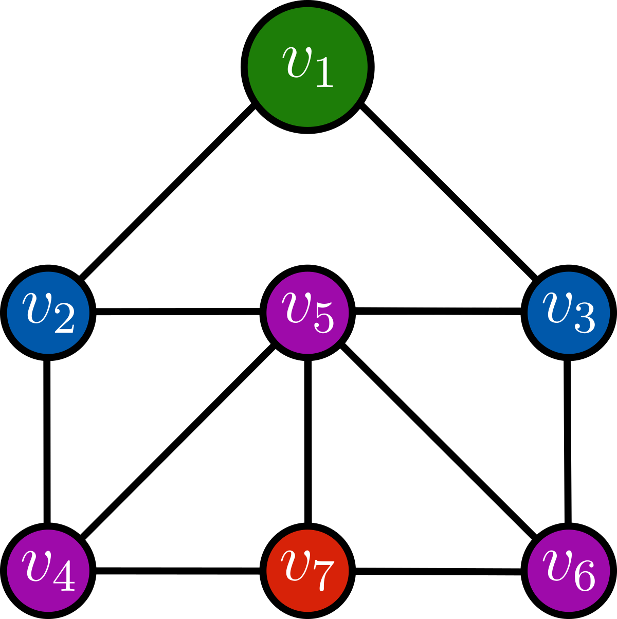
Let us consider the mesh $T(\mathcal{V},\mathcal{E},\mathcal{F})$, which can be seen as a simple, undirected, and connected graph $\mathcal{G}(\mathcal{V},\mathcal{E})$ with nodes $\mathcal{V}$ and edges $\mathcal{E}$ (see Figure 2), including additional information about the elements of the mesh $\mathcal{F}$.

The nodes have associated features $\mathbf{u}$, that represent the evaluation of a set of state variables at the vertices of the mesh. This information can be embedded in the matrix $\mathbf{U}=\left[\mathbf{u}_{1}|\dots|\mathbf{u}_{N_{h}}\right]^{T}\in\mathbb{R}^{N_{h}\times d}$, for all the $N_{h}$ nodes of the graph¹¹ 1 The dataset is obtained by extracting the values of the high-fidelity solutions at the corresponding vertexes of the mesh, regardless the polynomial order of the Lagrange elements., which have no particular order, and $d$ features, i.e. a scalar or vector field. The adjacency matrix $\mathbf{A}\in\mathbb{R}^{N_{h}\times N_{h}}$ records of the connections among nodes. A convenient way of expressing it is by means of the adjacency list, where the $k$-th entry, corresponding to $e_{k}\in\mathcal{E}$, is the pair $(i,j)$ denoting the existence of a link between $v_{i},v_{j}\in\mathcal{V}$. This is crucial to efficiently define operations which are permutation-invariant and equivariant. Thus, one can randomly permute the original ordering of the nodes induced by the mesh labelling without changing the final output. This is a key difference with standard CNNs, where a fixed filter produces different outputs if two pixels are swapped.

Starting from the graph structure as defined above, one obtains a graph neural network by defining a set of optimizable operations acting on all attributes of the graph. Despite their recent introduction, many works have focused on how to process graph-data through a neural network. Thus, let us review in more detail the basic operations which constitutes the backbone of many GNN architectures: (i) message passing framework, (ii) convolutional layers, and (iii) down-sampling and up-sampling procedures.

We are now ready to propose the graph convolutional autoencoder for model order reduction applications. The main sources of inspiration is CNN-based autoencoder architecture introduced in [30, 53]. As detailed in the previous sections, such approaches are particularly useful when dealing with structured meshes, that can be seen as images with a fixed number of neighboring pixels. For this reason, we consider a similar architecture, but extend its applicability in a geometrically consistent manner to unstructured meshes defined over complex domains, when a Cartesian representation is no longer possible.

ML approaches mimic the standard ROM setting, having an offline phase in which one forms the dataset and build the reduced model by training the neural network, and an online phase for the real-time evaluation of the field of interest.

We consider the graph dataset $\Xi=\{\textbf{u}_{\mathcal{N}}({\boldsymbol{\mu}}^{i}),\Omega_{{\mathcal{N}}}({\boldsymbol{\mu}}^{i})\}_{i=1}^{N_{\text{S}}}$, formed by $N_{\text{S}}$ solutions $\textbf{u}_{\mathcal{N}}({\boldsymbol{\mu}}^{i})$ of a parametrized PDE defined over unstructured meshes $\Omega_{{\mathcal{N}}}({\boldsymbol{\mu}}^{i})$, corresponding to the set of parameters $\{{\boldsymbol{\mu}}^{i}\}_{i=1}^{N_{\text{S}}}$. Following the first DL-ROM approach [30], we detail the steps of the modular architecture and refer to Figures 4 and 5, respectively, for the offline and online phases.

The architecture for the offline training is composed of an autoencoder and a multi-layer perceptron (MLP). The former seeks to approximate the identity map while encoding the information into a low-dimensional space expressed by the bottleneck or latent space.

We feed the encoder module $\phi_{\mathbf{W}}$ with the graph data $\Xi$, exploiting MoNet (5) as the message passing algorithm. In this step, by means of graph convolutions $g_{\mathbf{W}}*\mathbf{H}^{(k)}$, we extract the most meaningful information between the nodes and their evolution w.r.t. the samples. When interested in reducing the graph dimensionality, one can consider an additional module by applying a fixed random mask for down-sampling, to obtain a reduced graph with $\mathbf{H}_{r}^{(k)}$ hidden embeddings. A second batch of convolutional layers $g_{\mathbf{W}}*\mathbf{H}_{r}^{(k)}$ can be used to further encode the latent space. To improve training, we also augment the network with a residual learning strategy exploiting skip-connections, featuring identity shortcuts inspired by the ResNet framework developed in [42]. This step, which can only be applied in batches of convolutions sharing the same graph’s size, enables the architecture to acquire the residual knowledge between layers, while simultaneously promoting the flow of gradient information throughout the network. At this stage, we use fully-connected layers to connect the graph structure with the bottleneck. We thus encode the original information in the latent vector $\tilde{\mathbf{u}}_{N}({\boldsymbol{\mu}})\in\mathbb{R}^{N}$, obtained as the evaluation of the solution field through the encoder structure $\tilde{\mathbf{u}}_{N}({\boldsymbol{\mu}})=\phi_{\mathbf{W}}(\textbf{u}_{\mathcal{N}}({\boldsymbol{\mu}}))$. The decoding structure is composed by the same operations as the encoding ones, but in reversed order. This way, processing the bottleneck with the decoder $\psi_{\mathbf{W}}$, we obtain the reconstruction of the original field $\tilde{u}_{\mathcal{N}}({\boldsymbol{\mu}})=\psi_{\mathbf{W}}(\tilde{\mathbf{u}}_{N}({\boldsymbol{\mu}}))$, and we can assemble the first term in the loss function for the unsupervised learning task as

Having encoded the latent variables with the autoencoder, we use this dataset for the supervised learning task with the MLP. Thus, we are non-intrusively building the map $\textbf{u}_{N}({\boldsymbol{\mu}})=\text{MLP}({\boldsymbol{\mu}})$, from which we can recover the reduced coefficient. The MLP, fundamental for the online evaluation phase, defines the loss

These two Mean Squared Error (MSE) loss terms can be balanced through the hyperparameter $\lambda$, resulting in the loss function

which guides the training procedure through the Adam optimizer. Finally, during the online phase, the bottleneck can be directly evaluated by exploiting the MLP for a new parameter ${\boldsymbol{\mu}}$, and successively decompressed through the graph decoder, to recover the corresponding field defined over its geometry.

As for the preprocessing of the dataset, we applied a double normalization with respect to the sample and the features, i.e. we impose zero mean and unitary variance for each column (i.e. node-wise), and subsequently for each row (i.e. parameter-wise). This allowed us to treat all the benchmarks within a unique framework, greatly improving the results. Moreover, we split the dataset $\Xi$ into training and testing set w.r.t. the percentage rate $r_{\text{t}}$ in the following manner: $\Xi_{\text{tr}}=\mathsf{shuffled}({\Xi})[{:},{:}r_{\text{t}}N_{\text{S}}]$ and $\Xi_{\text{te}}=\Xi\setminus\Xi_{\text{tr}}$ of dimension $N_{\text{te}}$.

Common disadvantages of machine learning approaches are the tuning of the hyperparameter and the learning procedure. As we will show in Section 4, the GCA-ROM architecture is quite robust w.r.t. both. Among the possible quantities to be investigated we focus on the following set: the training rate percentage $r_{\text{t}}$, the pooling rate percentage $r_{\text{p}}$, the number of nodes in the feedforward network of the GCA ffn, the number of nodes in each MLP layer of the latent map $n_{l}$, the dimension of the bottleneck $n$, the weight $\lambda$ in the loss function, and the number of a-priori and a-posteriori hidden channels, hcp and hcd, respectively.

The scope of the hyperparameter analysis (showed in Appendix A.1) is not to produce the best possible accuracy for the model, but to explore the sensitivity of the architecture to different autoencoder configurations. For this reason, we have not focused on the usual ones, e.g. activation functions, learning rates and number of epochs, nor exploited multiple restart approaches with different seeds. In particular, we considered the combinations of the following configurations for the aforementioned hyperparameters³³ 3 In the pooling case, testing the architecture without convolutional layers is equivalent to learning the map only from sensors data.: $r_{\text{t}}\in[10,30,50]$, $r_{\text{p}}\in[30,50,70]$, $\text{ffn}\in[100,200,300]$, $n_{l}\in[50,100]$, $n\in[15,25]$, $\lambda\in[0.1,1,10]$, and $\text{hcp},\text{hcd}\in[1,2,3]$.

We remark that, as in CNNs, our GNN architecture shares the weights across the nodes⁴⁴ 4 The weights multiply the hidden embedding $\mathbf{h}_{u}^{(k)}$, thus the matrix $\mathbf{W}^{(k)}$ depends only on the number of features and filters, but not on the number of neighbors $|\mathsf{N}(u)|$. This allows for many possible generalizations, from different meshes to unseen nodes., making it scalable to large datasets, in contrast to fully-connected autoencoders. This results in a much lower number of trainable parameters, and substantial speed-up in the training phase. The size of the optimization problem is thus dominated by the MLP dimension. For this reason the pooling approach could be fundamental for finer meshes.

This geometry-informed architecture not only reduces the computational complexity, but also fosters learning. Indeed, already with a relatively small training horizon, i.e. $N_{\text{epochs}}=5000$, the network reaches accurate reconstruction errors for the benchmarks, and still show a decreasing behavior. Finally, we note that GCA-ROM is a convolve-then-reshape method, extracting the inductive bias directly from its original framework, while the ones exploiting standard CNNs are reshape-then-convolve approaches.

The first benchmark consists of a nonlinear elliptic problem in a two-dimensional hexagonal domain $\Omega$ with a hole, depicted in Figure 6. With this toy problem, we aim at testing the ability of GCA-ROM to cope with an unstructured mesh with $N_{h}=2562$ nodes, where the Euclidean geometry based on Cartesian coordinates does not provide a valid description of the domain.

The continuous formulation of the PDE governing this parametrized problem reads as: given $\boldsymbol{\mu}\in\mathbb{P}$, find $u(\boldsymbol{\mu})$ such that

where the physical multi-parameter $\boldsymbol{\mu}=(\mu_{1},\mu_{2})\in\mathbb{P}=[0.01,10]^{2}$ controls the strength of the sink term and of the nonlinearity, and the source term is characterized by the following expression

The dataset is constituted by $N_{\text{S}}=100$ snapshots (10 equispaced parameter samples in each direction) by means of Finite Element approximations over a uniform grid in $\mathbb{P}$. The nonlinear term prevents the straightforward applicability of ROMs (hyper-reduction techniques are needed to recover the efficiency), while the lack of a structured mesh leads to a geometrically inconsistent use of standard CNNs.

We show in Figure 7 the high-fidelity solution for Poisson obtained for $\boldsymbol{\mu}=(3.34,4.45)\in\Xi_{\text{te}}$, and the GCA-ROM relative errors obtained with and without exploiting pooling procedures. In both cases, we can accurately reconstruct the corresponding field, with the pooling architecture performing slightly worse due to the high peaks in some regions of the domain, $\varepsilon_{\text{GCA}}(\boldsymbol{\mu})=5.0\times 10^{-3}$ and $\varepsilon_{\text{GCA}}(\boldsymbol{\mu})=4.3\times 10^{-3}$, respectively for pooling and plain versions. This is expected given the availability of only partial information over the solution field during the training stage.

In Figure 7(b), the error is higher near the maxima of the field, where the dataset $\Xi$ shows the higher variance w.r.t. the sampling, and at the boundary of the domain. This is clearly an undesired effect of the convolution procedure, sharing the message with neighbors even where we impose homogeneous Dirichlet boundary conditions. However, this effect is only present for a few instances of the parameter, while in general the error is spatially distributed in the whole domain, confirming that, regardless the complexity of the solution manifold, GCA-ROM learns the intrinsic behavior and generalize to unseen data. The augmentation of our data-driven architecture with physical information can fix such behavior by guiding the learning task towards physically consistent fields, and will be the subject of forthcoming investigations. With the pooling approach, see Figure 7(c), the accuracy drops especially near the down-sampled regions, where we apply the mask.

To highlight the generalization capabilities achieved by GCA-ROM, we show in Figure 8, for both approaches, the evolution of the relative error $\varepsilon_{GCA}(\boldsymbol{\mu})$ in the whole dataset $\Xi$. As expected, the accuracy of the pooling approach, both in terms of mean and maximum errors, marginally deteriorates due to the lack of information, but still produces remarkably close results. For the plain architecture in Figure 8(a), it can be seen that, exploiting only $r_{\text{t}}=30\%$ of the original dataset (reported in the plot with red stars), the relative error over $\Xi_{\text{te}}$ is below $2\times 10^{-2}$ and its mean is $\overline{\varepsilon}_{GCA}=8\times 10^{-3}$. The accuracy of the pooling procedure in Figure 8(b) is also surprisingly good, again exploiting only $r_{\text{t}}=30\%$ of the dataset, but also retaining only $r_{\text{p}}=70\%$ of each high-fidelity solution, i.e. we do not have access to these fixed nodes. We are still able to reconstruct the Poisson solutions with maximum relative error below $2.7\times 10^{-2}$ and mean $\overline{\varepsilon}_{GCA}=1\times 10^{-2}$.

This result shows the potential of graph convolutional architecture in capturing parametric behavior, even when dealing with sparse measurements, and paves the way for the development of robust up- and down-sampling procedures.

Standard projection-based reduced order models struggle with slow Kolmogorov decay phenomena, such as those in the advection-dominated regime. Here, we test the performance of our nonlinear and data-driven approach for an advection-diffusion equation with a parametrized transport term. The domain is given by the unstructured mesh defined over the square domain $\Omega=[0,1]^{2}\in\mathbb{R}^{2}$, depicted in Figure 9, with $N_{h}=3967$ nodes.

The advection-dominated problem reads as: given $\boldsymbol{\mu}\in\mathbb{P}$, find $u(\boldsymbol{\mu})$ such that

where $\alpha(\mu_{1})=10^{-\mu_{1}}$ represents the diffusion coefficient defining the Péclet number, $\beta(\mu_{2})=(\mu_{2},\mu_{2})$ is the direction of the transport, and $g=1$ is the source term. Thus, the model is characterized by the physical multi-parameter $\boldsymbol{\mu}=(\mu_{1},\mu_{2})\in\mathbb{P}=[0,6]\times[-1,1]$. As before, we form the dataset by means of $N_{\text{S}}=100$ snapshots over a uniform grid in $\mathbb{P}$.

In Figure 10 we plot the solution of the advection dominated problem for $\boldsymbol{\mu}=(2.67,0.33)\in\Xi_{\text{te}}$, and the two GCA-ROM relative error fields. Again, the qualitative behavior of the methodology shows accurate reconstructions, with the maximum errors located near the boundary layer’s region. Given the different amount of information, the error in Figure 10(b) is more distributed over the domain, and one order of magnitude smaller than the one in Figure 10(c).

For the accuracy, we plot in Figure 11 the relative errors $\varepsilon_{GCA}(\boldsymbol{\mu})$ in the plain and down-sampled architectures over the dataset $\Xi$. In both cases, the training set comprises only $r_{\text{t}}=30\%$ of the computed snapshots, but the maximum relative error over $\Xi_{\text{te}}$ is around $5.2\times 10^{-2}$, while its mean is $\overline{\varepsilon}_{GCA}=2.4\times 10^{-2}$. We stress the fact that to learn this complex behavior, we are only exploiting 30 high-fidelity solutions fixed a-priori by the seed, and testing on the remaining 70. The pooling strategy gives comparable results by selecting $r_{\text{p}}=70\%$ nodes, and thus masking $30\%$ of them, with maximum relative error below $7.2\times 10^{-2}$ and mean $\overline{\varepsilon}_{GCA}=3.3\times 10^{-2}$.

The graph structure is thus still able to predict unseen patterns, even when dealing with a combination of: a low-data regime, scattered mesh information, and complex parametric behavior compromising the linear reducibility of the model.

One of the main advantages of the GCA-ROM architecture is the possibility to work directly on the (unstructured) computational domain, introducing geometric priors and defining physically consistent convolutional operations. Now, we consider the case in which the PDE is posed on a geometrically parametrized domain⁵⁵ 5 The geometric parametrization is performed w.r.t. affine mappings, thus producing a set of snapshots defined on the same number of nodes as the original mesh cardinality., i.e. when the distance between nodes changes w.r.t. the parameter. Standard convolutions are agnostic to this behavior. We study a steady-state Graetz problem on the parametrized rectangular geometry $\Omega(\mu_{1})=\Omega_{1}\cup\Omega_{2}(\mu_{1})\in\mathbb{R}^{2}$ depicted in Figure 12, with $\Omega_{1}=[0,1]\times[0,1]$ and $\Omega_{2}=[0,\mu_{1}]\times[0,1]$, and discretized with $N_{h}=5160$ nodes.

The Graetz model describes a thermal field under the combined effects of heat’s diffusion and advection along the horizontal direction, with homogeneous and non-homogeneous boundary conditions. The continuous PDE’s formulation of the Graetz problem reads as: given $\boldsymbol{\mu}\in\mathbb{P}$, find $u(\boldsymbol{\mu})$ such that

where $\boldsymbol{n}$ denotes the outer normal to the boundary $\Gamma_{\text{N}}$. We impose homogeneous Dirichlet conditions on $\Gamma_{\text{D}}=\Gamma_{1}\cup\Gamma_{5}\cup\Gamma_{6}$, while the temperature is kept at $u=1$ at the boundaries $\Gamma_{\text{G}}=\Gamma_{2}(\mu_{1})\cup\Gamma_{4}(\mu_{1})$. Finally, homogeneous Neumann conditions are imposed on $\Gamma_{\text{N}}=\Gamma_{3}(\mu_{1})$.

The model has been parametrized by means of a physical and geometrical multi-parameter $\boldsymbol{\mu}=(\mu_{1},\mu_{2})\in\mathbb{P}=[1,3]\times[0.01,0.1]$, controlling the length $\mu_{1}$ of the idealized pipes, and the diffusivity coefficient $\mu_{2}$. The dataset is formed by $N_{\text{S}}=200$ snapshots, computed on a uniform grid in $\mathbb{P}$ with respectively 10 and 20 equispaced values for the two parameters.

In Figure 13 we plot the solution of the Graetz model obtained for $\boldsymbol{\mu}=(2.78,0.01)\in\Xi_{\text{te}}$, comparing the relative errors for two GCA-ROM approaches. The error in Figure 13(b) has a maximum in the center of the stretched subdomain, where the transport phenomena takes place, while the pooling approach in Figure 13(c) produces higher errors at the interface between the two boundary conditions.

Figure 14 shows the investigation of the reconstruction accuracy over the dataset $\Xi$ through the relative errors $\varepsilon_{GCA}(\boldsymbol{\mu})$. The plain GCA-ROM architecture is still able to learn the low-dimensional evolution in the context of a varying geometry by exploiting only $r_{\text{t}}=30\%$ of the dataset information, with the relative error over $\Xi_{\text{te}}$ always below $6.7\times 10^{-2}$, with mean $\overline{\varepsilon}_{GCA}=5.6\times 10^{-3}$. The results for the pooling approach are again comparable, with maximum relative error below $9.3\times 10^{-2}$ and mean $\overline{\varepsilon}_{GCA}=7\times 10^{-3}$, when exploiting $r_{\text{p}}=70\%$ of the mesh. In both cases, we observe high generalization accuracy of the GCA-ROM in capturing the geometric parametrization. This is a result of the introduction of the geometric priors through the GNN architecture endowed with the MoNet convolutional layers. The higher errors are indeed localized for smaller values of the diffusivity parameter, where the phenomenon approaches the advection dominated regime.

As the last benchmark, we consider a more complex problem that combines nonlinear terms, parametrized geometry and a vector unknown with non-unique solutions. The so-called Coanda’s effect in the Navier-Stokes system is a typical example of fluid dynamic bifurcation problem [67, 68, 48, 81]. For such problems, a small variation of the viscosity, in the neighborhood of the bifurcation points, produces a sudden change in the qualitative behavior of the solution, causing the co-existence of different states for the same parameter value. Here, we are not interested in recovering all the possible solutions. Rather, we seek to investigate the GCA-ROM performance in the approximation of the transition between two qualitatively different stable states, i.e. the symmetric flux and the wall-hugging profile.

We study the steady-state Navier-Stokes system on a parametrized sudden-expansion channel geometry $\Omega(\mu_{1})$, depicted in Figure 15, discretized with $N_{h}=2719$ nodes.

The continuous formulation of the Navier-Stokes problem reads as: given $\boldsymbol{\mu}\in\mathbb{P}$, find the velocity and pressure fields $\textbf{u}(\boldsymbol{\mu})=(u_{x}(\boldsymbol{\mu}),u_{y}(\boldsymbol{\mu}))$ and $p(\boldsymbol{\mu})$, such that

where n is the normal unit vector, $\mu_{1}$ is the half-width of the inlet channel, $\mu_{2}$ the kinematic viscosity of the fluid, and $\textbf{u}_{\text{in}}(\boldsymbol{x})=\begin{bmatrix}20(5-y)(y-2.5),\ 0\end{bmatrix}$ the Poiseuille inflow profile.

The Navier-Stokes benchmark is parametrized by means of the physical and geometric multi-parameter $\boldsymbol{\mu}=(\mu_{1},\mu_{2})\in\mathbb{P}=[0.5,2]^{2}$. The parametric investigation of this model is physically interesting, and the bifurcation point depends on the physical and geometrical flow’s configuration. This means that being able to predict the evolution of the bifurcation point in the parameter space allows to detect the changes in the stability properties of the system.

Given the nature of the model, with velocity and the pressure fields as unknowns, we show the adaptability of the architecture to vector problems. Thus, we consider a monolithic approach, where the three fields are concatenated as features for each node, rather than a partitioned one, where we recover independently each field⁶⁶ 6 Notice that this is possible given the data-driven nature of the architecture, i.e. we are not exploiting the physics coming from the PDE as in projection-based models..

We report in Table 1 the parametric setting for this benchmark. We highlight that the reason for such a high number of snapshots, $N_{\text{S}}=3171$, is that the Finite Element approximation of the bifurcating phenomenon requires a continuation technique to follow the symmetry-breaking branch [66]. Despite the increased cardinality of the sampling w.r.t. the former test cases, we fixed the training rate to only consider $r_{\text{t}}=10\%$ of the original dataset.

In Figure 16 we plot the three components of the Navier-Stokes solution for $\boldsymbol{\mu}=(0.57,0.57)\in\Xi_{\text{te}}$, and the GCA-ROM relative errors w.r.t. the high-fidelity snapshots. The errors are mainly localized in the regions where the flow suddenly changes, and among the three components, the vertical velocity is the one reconstructed least accurately. The components recover the wall-hugging behavior with the flow attaching to the bottom boundary, upon which we built the dataset.

On one side, we notice that this could still be considered a low-data regime, especially in the bifurcating context, while on the other this shows that the architecture can benefit when increasing the cardinality of $\Xi_{\text{tr}}$ without overfitting. As observed previously, the vertical velocity field is the most difficult to approximate, due to the fact that it is the component responsible for the symmetry breaking phenomenon, and thus the bifurcation. Higher generalization errors occur again for smaller values of the viscosity. For the vertical velocity, this is maximized for bigger inlet’s width, since in that region the geometry still does not admit the wall-hugging profile, while the (bifurcation-agnostic) data-driven approach is influenced by the neighboring training snapshots.

In this section, we compare the performance of GCA-ROM with standard linear techniques based on POD, and the original nonlinear DL-ROM architecture. Rather than focusing on the best case scenario, we detail the key features and main drawbacks of these approaches, considering the three scalar benchmarks previously discussed. As metrics, we do not only consider the mean relative error over the testing dataset $\Xi_{\text{te}}$, but also the offline and online timings, as well as the dimension of the optimization problem.

In Table 2, we report the accuracy over $\Xi_{\text{te}}$ of the different methodologies when trained on the same set of snapshots $\Xi_{\text{tr}}$ with $r_{\text{t}}=30\%$. To have a fair comparison, i.e. based on the same amount of information, we considered the GCA-ROM architecture without down-sampling, and we fixed the reduced/latent dimension to $n=15$ for all benchmarks and methodologies.

In particular, we consider the projection error in the POD space, denoted with (POD), the standard POD-Galerkin approach (POD-G), DL-ROM and GCA-ROM. As expected, when considering a large enough latent dimension, thanks to the exponential decay of the reduced error, projecting in the POD space gives the best results in terms of approximation accuracy. POD-G still produces better performance as compared to ML-based techniques (at least for large enough values of $n$) when dealing with easily reducible problems, such as Poisson or Graetz.

On the contrary, nonlinear techniques show greater capabilities when dealing with advection-dominated phenomena, which are characterized by a slow Kolmogorov $n$-width decay. In all cases, GCA-ROM provided better results than its CNN-based counterpart, even beating the POD-G approach for the Advection test case. This confirms that augmenting the learning procedure with geometrical biases helps the optimization step.

Other non-intrusive POD-based approaches, such as POD-NN or PODI, have been investigated, but the low-data regime we are interested in is a well-known issue for these methodologies. Indeed, both non-intrusive regression and interpolation approaches usually require a large training dataset, without which the learning capabilities are compromised, and the model is unable to generalize.

As an example, we show the DL-ROM results for the geometrically parametrized Graetz problem. Relying on an affine map transformation between the original and reference domains, this corresponds to the easiest setting in which to investigate the performance for unstructured grids in advanced applications. In Figure 19 we plot the relative error of the DL-ROM approach $\varepsilon_{DL}(\boldsymbol{\mu})$, and the solution and error fields of the Graetz model obtained for $\boldsymbol{\mu}=(1,0.03)\in\Xi_{\text{te}}$. While the original approach is still able to learn the main features of the model, with possible implications still to be understood [89, 28], and a mean $\overline{\varepsilon}_{DL}=1.6\times 10^{-2}$, we notice that it also produces an unsatisfactory maximum one around $1.4\times 10^{-1}$. This is localized in the area corresponding to the maximum stretching for the domain, where the geometric consistency is even more crucial.

Furthermore, given the non-locality of the convolutional operator in DL-ROM, the reconstruction of the solution field is in general not smooth, as the one depicted in Figure 19. The error shows a speckled pattern affecting the solution in its entire domain, and producing an oscillating reconstruction of the thermal field. Comparing the results with the ones in Figure 13, the same effect is much less evident, producing a smooth field even considering a highly deformed geometrical configuration and a lower viscosity value.

As regard the efficiency, we now discuss both the offline and online complexity of the two methodologies. While the GCA-ROM approach takes as input the high-fidelity fields already defined on their unstructured geometry, DL-ROM approaches require reshaping the data as a matrix, applying a padding strategy to reach the desired dimensions and apply convolution. This artificial addition of zeroes could potentially compromise the learning procedure, as well as increasing its computational complexity.

In Table 3 we compare GCA-ROM and DL-ROM in terms of training and testing times, and number of parameters involved in the optimization process. It is worth noting that message passing is a computationally demanding operation for GNNs, but exploiting local convolutions in such context, the sharing of weights reduce significantly the amount of learnable parameters in the network. Depending on the dimension of the filters, we notice a reduction of order three to four. Indeed, the amount of weights exploited by DL-ROM heavily depends on the filter sizes, while for GCA-ROM it is almost the same, i.e. the cost of the weighting functions in the Gaussian kernels of MoNet is dominated by the one of the feed-forward layer. For this reason, a more in depth investigation of the up-sampling and down-sampling procedures, could drastically improve the efficiency of the presented methodology.

All simulations have been performed on a workstation equipped with an Nvidia Quadro GP100 GPU. We report both CPU and GPU times, showing that GCA-ROM is computationally affordable even when only modest hardware is available⁷⁷ 7 We remark that computational GPU times in the GCA-ROM setting can be further optimized by exploiting new releases of PyTorch Geometric, enabling even faster computations.. Testing times are including the computation of the reconstructed solutions for all the parameter values in $\Xi$.

References

- [1] D. Amsallem, M. J. Zahr, and C. Farhat. Nonlinear model order reduction based on local reduced-order bases. International Journal for Numerical Methods in Engineering, 92(10):891–916, 2012.
- [2] P. F. Antonietti, N. Farenga, E. Manuzzi, G. Martinelli, and L. Saverio. Agglomeration of Polygonal Grids using Graph Neural Networks with applications to Multigrid solvers. arXiv preprint arXiv:2210.17457, 2023.
- [3] J. L. Barnett, C. Farhat, and Y. Maday. Neural-Network-Augmented Projection-Based Model Order Reduction for Mitigating the Kolmogorov Barrier to Reducibility of CFD Models. arXiv preprint arXiv:2212.08939, 2022.
- [4] M. Barrault, N. C. Nguyen, Y. Maday, and A. T. Patera. An “empirical interpolation” method: Application to efficient reduced-basis discretization of partial differential equations. C. R. Acad. Sci. Paris, Série I., 339:667–672, 2004.
- [5] S. Barwey, V. Shankar, V. Viswanathan, and R. Maulik. Multiscale Graph Neural Network Autoencoders for Interpretable Scientific Machine Learning. arXiv preprint arXiv:2302.06186, 2023.
- [6] P. W. Battaglia, J. B. Hamrick, V. Bapst, A. Sanchez-Gonzalez, V. Zambaldi, M. Malinowski, A. Tacchetti, D. Raposo, A. Santoro, R. Faulkner, et al. Relational inductive biases, deep learning, and graph networks. arXiv preprint arXiv:1806.01261, 2018.
- [7] P. Benner, A. Cohen, M. Ohlberger, and K. Willcox. Model Reduction and Approximation: Theory and Algorithms. Computational Science and Engineering Series. SIAM, Society for Industrial and Applied Mathematics, 2017.
- [8] P. Benner, S. Grivet Talocia, A. Quarteroni, G. Rozza, W. Schilders, and L. M. Silveira. Model Order Reduction, volume 1-3. De Gruyter, 2020.
- [9] S. Berrone, F. Della Santa, A. Mastropietro, S. Pieraccini, and F. Vaccarino. Graph-Informed Neural Networks for Regressions on Graph-Structured Data. Mathematics, 10(5):786, 2022.
- [10] F. M. Bianchi, D. Grattarola, and C. Alippi. Spectral clustering with graph neural networks for graph pooling. In International Conference on Machine Learning, pages 874–883. PMLR, 2020.
- [11] M. M. Bronstein, J. Bruna, T. Cohen, and P. Veličković. Geometric deep learning: grids, groups, graphs, geodesics, and gauges. arXiv preprint arXiv:2104.13478, 2021.
- [12] T. Bui-Thanh, M. Damodaran, and K. Willcox. Proper Orthogonal Decomposition Extensions for Parametric Applications in Compressible Aerodynamics. In 21st AIAA Applied Aerodynamics Conference, Fluid Dynamics and Co-located Conferences. American Institute of Aeronautics and Astronautics, 2003.
- [13] C. Cangea, P. Veličković, N. Jovanović, T. Kipf, and P. Liò. Towards sparse hierarchical graph classifiers. arXiv preprint arXiv:1811.01287, 2018.
- [14] S. Chaturantabut and D. C. Sorensen. Nonlinear model reduction via discrete empirical interpolation. SIAM Journal on Scientific Computing, 32(5):2737–2764, 2010.
- [15] W. Chen, Q. Wang, J. S. Hesthaven, and C. Zhang. Physics-informed machine learning for reduced-order modeling of nonlinear problems. Journal of Computational Physics, 446:110666, 2021.
- [16] P. G. Ciarlet. Linear and Nonlinear Functional Analysis with Applications. Other Titles in Applied Mathematics. Society for Industrial and Applied Mathematics, 2013.
- [17] L. Cicci, S. Fresca, and A. Manzoni. Deep-HyROMnet: A Deep Learning-Based Operator Approximation for Hyper-Reduction of Nonlinear Parametrized PDEs. Journal of Scientific Computing, 93(2):57, 2022.
- [18] D. Coscia, L. Meneghetti, N. Demo, G. Stabile, and G. Rozza. A continuous convolutional trainable filter for modelling unstructured data. arXiv preprint arXiv:2210.13416, 2022.
- [19] M. Defferrard, X. Bresson, and P. Vandergheynst. Convolutional neural networks on graphs with fast localized spectral filtering. Advances in neural information processing systems, 29, 2016.
- [20] N. Demo, M. Tezzele, and G. Rozza. A non-intrusive approach for the reconstruction of POD modal coefficients through active subspaces. Comptes Rendus Mécanique, 347(11):873–881, 2019.
- [21] N. Demo, M. Tezzele, and G. Rozza. A DeepONet Multi-Fidelity Approach for Residual Learning in Reduced Order Modeling. arXiv preprint arXiv:2302.12682, 2023.
- [22] P. Díez, A. Muixí, S. Zlotnik, and A. García-González. Nonlinear dimensionality reduction for parametric problems: A kernel proper orthogonal decomposition. International Journal for Numerical Methods in Engineering, 122(24):7306–7327, 2021.
- [23] K. Doherty, C. Simpson, S. Becker, and A. Doostan. QuadConv: Quadrature-Based Convolutions with Applications to Non-Uniform PDE Data Compression. arXiv preprint arXiv:2211.05151, 2023.
- [24] V. Ehrlacher, D. Lombardi, O. Mula, and F.-X. Vialard. Nonlinear model reduction on metric spaces. Application to one-dimensional conservative PDEs in Wasserstein spaces. ESAIM: Mathematical Modelling and Numerical Analysis, 54(6):2159–2197, 2020.
- [25] FEniCS. https://www.fenicsproject.org.
- [26] M. Fey and J. E. Lenssen. Fast graph representation learning with PyTorch Geometric. In ICLR Workshop on Representation Learning on Graphs and Manifolds, 2019.
- [27] M. Fortunato, T. Pfaff, P. Wirnsberger, A. Pritzel, and P. Battaglia. MultiScale MeshGraphNets. arXiv preprint arXiv:2210.00612, 2022.
- [28] N. R. Franco, S. Fresca, A. Manzoni, and P. Zunino. Approximation bounds for convolutional neural networks in operator learning. Neural Networks, 161:129–141, 2023.
- [29] N. R. Franco, A. Manzoni, and P. Zunino. Learning Operators with Mesh-Informed Neural Networks. arXiv preprint arXiv:2203.11648, 2022.
- [30] S. Fresca, L. Dede, and A. Manzoni. A comprehensive deep learning-based approach to reduced order modeling of nonlinear time-dependent parametrized PDEs. Journal of Scientific Computing, 87(2):1–36, 2021.
- [31] S. Fresca and A. Manzoni. POD-DL-ROM: enhancing deep learning-based reduced order models for nonlinear parametrized PDEs by proper orthogonal decomposition. Computer Methods in Applied Mechanics and Engineering, 388:114181, 2022.
- [32] H. Gao and S. Ji. Graph U-nets. In international conference on machine learning, pages 2083–2092. PMLR, 2019.
- [33] H. Gao, M. J. Zahr, and J.-X. Wang. Physics-informed graph neural Galerkin networks: A unified framework for solving PDE-governed forward and inverse problems. Computer Methods in Applied Mechanics and Engineering, 390:114502, 2022.
- [34] R. J. Gladstone, H. Rahmani, V. Suryakumar, H. Meidani, M. D’Elia, and A. Zareei. GNN-based physics solver for time-independent PDEs. arXiv preprint arXiv:2303.15681, 2023.
- [35] D. Grattarola, D. Zambon, F. M. Bianchi, and C. Alippi. Understanding pooling in graph neural networks. IEEE Transactions on Neural Networks and Learning Systems, 2022.
- [36] C. Greif and K. Urban. Decay of the Kolmogorov N-width for wave problems. Applied Mathematics Letters, 96:216–222, 2019.
- [37] A. Gruber, M. Gunzburger, L. Ju, and Z. Wang. A comparison of neural network architectures for data-driven reduced-order modeling. Computer Methods in Applied Mechanics and Engineering, 393:114764, 2022.
- [38] M. Guo and J. S. Hesthaven. Reduced order modeling for nonlinear structural analysis using Gaussian process regression. Computer Methods in Applied Mechanics and Engineering, 341:807–826, 2018.
- [39] W. Hamilton, Z. Ying, and J. Leskovec. Inductive representation learning on large graphs. Advances in neural information processing systems, 30, 2017.
- [40] W. L. Hamilton. Graph representation learning. Synthesis Lectures on Artificial Intelligence and Machine Learning, 14(3):1–159, 2020.
- [41] X. Han, H. Gao, T. Pffaf, J.-X. Wang, and L.-P. Liu. Predicting physics in mesh-reduced space with temporal attention. arXiv preprint arXiv:2201.09113, 2022.
- [42] K. He, X. Zhang, S. Ren, and J. Sun. Deep residual learning for image recognition. In Proceedings of the IEEE conference on computer vision and pattern recognition, pages 770–778, 2016.
- [43] Q. Hernandez, A. Badias, F. Chinesta, and E. Cueto. Thermodynamics-informed graph neural networks. IEEE Transactions on Artificial Intelligence, 2022.
- [44] Q. Hernandez, A. Badias, D. Gonzalez, F. Chinesta, and E. Cueto. Deep learning of thermodynamics-aware reduced-order models from data. Computer Methods in Applied Mechanics and Engineering, 379:113763, 2021.
- [45] J. S. Hesthaven, G. Rozza, and B. Stamm. Certified Reduced Basis Methods for Parametrized Partial Differential Equations. SpringerBriefs in Mathematics. Springer International Publishing AG, Cham, 1st ed. 2016 edition, 2015.
- [46] J. S. Hesthaven and S. Ubbiali. Non-intrusive reduced order modeling of nonlinear problems using neural networks. Journal of Computational Physics, 363:55–78, 2018.
- [47] A. Kashefi, D. Rempe, and L. J. Guibas. A point-cloud deep learning framework for prediction of fluid flow fields on irregular geometries. Physics of Fluids, 33(2):027104, 2021.
- [48] M. Khamlich, F. Pichi, and G. Rozza. Model order reduction for bifurcating phenomena in fluid-structure interaction problems. International Journal for Numerical Methods in Fluids, 94(10):1611–1640, 2022.
- [49] Y. Kim, Y. Choi, D. Widemann, and T. Zohdi. A fast and accurate physics-informed neural network reduced order model with shallow masked autoencoder. Journal of Computational Physics, 451:110841, 2022.
- [50] T. N. Kipf and M. Welling. Semi-supervised classification with graph convolutional networks. arXiv preprint arXiv:1609.02907, 2016.
- [51] J. Kneifl, D. Rosin, O. Röhrle, and J. Fehr. Low-dimensional Data-based Surrogate Model of a Continuum-mechanical Musculoskeletal System Based on Non-intrusive Model Order Reduction. arXiv preprint arXiv:2302.06528, 2023.
- [52] N. Kovachki, Z. Li, B. Liu, K. Azizzadenesheli, K. Bhattacharya, A. Stuart, and A. Anandkumar. Neural operator: Learning maps between function spaces. arXiv preprint arXiv:2108.08481, 2021.
- [53] K. Lee and K. T. Carlberg. Model reduction of dynamical systems on nonlinear manifolds using deep convolutional autoencoders. Journal of Computational Physics, 404:108973, 2020.
- [54] C. Liu, Y. Zhan, C. Li, B. Du, J. Wu, W. Hu, T. Liu, and D. Tao. Graph pooling for graph neural networks: Progress, challenges, and opportunities. arXiv preprint arXiv:2204.07321, 2022.
- [55] L. Lu, P. Jin, G. Pang, Z. Zhang, and G. E. Karniadakis. Learning nonlinear operators via DeepONet based on the universal approximation theorem of operators. Nature Machine Intelligence, 3(3):218–229, 2021.
- [56] R. Maulik, B. Lusch, and P. Balaprakash. Reduced-order modeling of advection-dominated systems with recurrent neural networks and convolutional autoencoders. Physics of Fluids, 33(3):037106, 2021.
- [57] M. Milano and P. Koumoutsakos. Neural Network Modeling for Near Wall Turbulent Flow. Journal of Computational Physics, 182(1):1–26, 2002.
- [58] F. Monti, D. Boscaini, J. Masci, E. Rodola, J. Svoboda, and M. M. Bronstein. Geometric deep learning on graphs and manifolds using mixture model cnns. In Proceedings of the IEEE conference on computer vision and pattern recognition, pages 5115–5124, 2017.
- [59] M. Morimoto, K. Fukami, K. Zhang, A. G. Nair, and K. Fukagata. Convolutional neural networks for fluid flow analysis: toward effective metamodeling and low dimensionalization. Theoretical and Computational Fluid Dynamics, 35(5):633–658, 2021.
- [60] B. Moya, A. Badias, D. Gonzalez, F. Chinesta, and E. Cueto. Physics perception in sloshing scenes with guaranteed thermodynamic consistency. IEEE Transactions on Pattern Analysis and Machine Intelligence, 2022.
- [61] M. Ohlberger and S. Rave. Nonlinear reduced basis approximation of parameterized evolution equations via the method of freezing. Comptes Rendus Mathematique, 351(23):901–906, 2013.
- [62] S. Pawar, S. E. Ahmed, O. San, and A. Rasheed. Data-driven recovery of hidden physics in reduced order modeling of fluid flows. Physics of Fluids, 32(3):036602, 2020.
- [63] L. Pegolotti, M. R. Pfaller, N. L. Rubio, K. Ding, R. B. Brufau, E. Darve, and A. L. Marsden. Learning Reduced-Order Models for Cardiovascular Simulations with Graph Neural Networks. arXiv preprint arXiv:2303.07310, 2023.
- [64] B. Peherstorfer and K. Willcox. Data-driven operator inference for nonintrusive projection-based model reduction. Computer Methods in Applied Mechanics and Engineering, 306:196–215, 2016.
- [65] J.-Z. Peng, S. Chen, N. Aubry, Z. Chen, and W.-T. Wu. Unsteady reduced-order model of flow over cylinders based on convolutional and deconvolutional neural network structure. Physics of Fluids, 32(12):123609, 2020.
- [66] F. Pichi. Reduced order models for parametric bifurcation problems in nonlinear PDEs. PhD thesis, Scuola Internazionale Superiore di Studi Avanzati, 2020.
- [67] F. Pichi, F. Ballarin, G. Rozza, and J. S. Hesthaven. An artificial neural network approach to bifurcating phenomena in computational fluid dynamics. Computers & Fluids, 254:105813, 2023.
- [68] F. Pichi, M. Strazzullo, F. Ballarin, and G. Rozza. Driving bifurcating parametrized nonlinear PDEs by optimal control strategies: Application to Navier–Stokes equations with model order reduction. ESAIM: Mathematical Modelling and Numerical Analysis, 56(4):1361–1400, 2022.
- [69] C. R. Qi, L. Yi, H. Su, and L. J. Guibas. Pointnet++: Deep hierarchical feature learning on point sets in a metric space. Advances in neural information processing systems, 30, 2017.
- [70] J. Qin, L. Liu, H. Shen, and D. Hu. Uniform pooling for graph networks. Applied Sciences, 10(18):6287, 2020.
- [71] A. Quarteroni, A. Manzoni, and F. Negri. Reduced Basis Methods for Partial Differential Equations: An Introduction. La Matematica per Il 3+2, 92. Springer International Publishing, Cham, 1st ed. 2016. edition, 2016.
- [72] A. Ranjan, T. Bolkart, S. Sanyal, and M. J. Black. Generating 3d faces using convolutional mesh autoencoders. In Proceedings of the European Conference on Computer Vision (ECCV), pages 704–720, 2018.
- [73] RBniCS. https://www.rbnicsproject.org.
- [74] J. Reiss, P. Schulze, J. Sesterhenn, and V. Mehrmann. The Shifted Proper Orthogonal Decomposition: A Mode Decomposition for Multiple Transport Phenomena. SIAM Journal on Scientific Computing, 40(3):A1322–A1344, 2018.
- [75] F. Romor, G. Stabile, and G. Rozza. Non-linear Manifold Reduced-Order Models with Convolutional Autoencoders and Reduced Over-Collocation Method. Journal of Scientific Computing, 94(3):74, 2023.
- [76] A. Sanchez-Gonzalez, J. Godwin, T. Pfaff, R. Ying, J. Leskovec, and P. Battaglia. Learning to simulate complex physics with graph networks. In International Conference on Machine Learning, pages 8459–8468. PMLR, 2020.
- [77] A. Sharma, E. Vans, D. Shigemizu, K. A. Boroevich, and T. Tsunoda. Deepinsight: A methodology to transform a non-image data to an image for convolution neural network architecture. Scientific reports, 9(1):1–7, 2019.
- [78] J. Shi and J. Malik. Normalized cuts and image segmentation. IEEE Transactions on pattern analysis and machine intelligence, 22(8):888–905, 2000.
- [79] J. Suk, P. de Haan, P. Lippe, C. Brune, and J. M. Wolterink. Mesh Neural Networks for SE(3)-Equivariant Hemodynamics Estimation on the Artery Wall. arXiv preprint arXiv:2212.05023, 2022.
- [80] T. Taddei. A Registration Method for Model Order Reduction: Data Compression and Geometry Reduction. SIAM Journal on Scientific Computing, 42(2):A997–A1027, 2020.
- [81] N. Tonicello, A. Lario, G. Rozza, and G. Mengaldo. Non-intrusive reduced order models for the accurate prediction of bifurcating phenomena in compressible fluid dynamics. arXiv preprint arXiv:2212.10198, 2022.
- [82] R. Vinuesa and S. L. Brunton. Enhancing computational fluid dynamics with machine learning. Nature Computational Science, 2(6):358–366, 2022.
- [83] S. Volkwein. Model reduction using proper orthogonal decomposition. Lecture Notes, Institute of Mathematics and Scientific Computing, University of Graz, 1025, 2011.
- [84] Y. Wang, Y. Sun, Z. Liu, S. E. Sarma, M. M. Bronstein, and J. M. Solomon. Dynamic graph cnn for learning on point clouds. Acm Transactions On Graphics (tog), 38(5):1–12, 2019.
- [85] P. Wu, S. Gong, K. Pan, F. Qiu, W. Feng, and C. Pain. Reduced order model using convolutional auto-encoder with self-attention. Physics of Fluids, 33(7):077107, 2021.
- [86] Z. Wu, S. Pan, F. Chen, G. Long, C. Zhang, and S. Y. Philip. A comprehensive survey on graph neural networks. IEEE transactions on neural networks and learning systems, 32(1):4–24, 2020.
- [87] J. Xu and L. Zikatanov. Algebraic multigrid methods. Acta Numerica, 26:591–721, 2017.
- [88] M. Xu, S. Song, X. Sun, and W. Zhang. A convolutional strategy on unstructured mesh for the adjoint vector modeling. Physics of Fluids, 33(3):036115, 2021.
- [89] C. Zhang, S. Bengio, M. Hardt, B. Recht, and O. Vinyals. Understanding deep learning (still) requires rethinking generalization. Communications of the ACM, 64(3):107–115, 2021.
- [90] J. Zhou, G. Cui, S. Hu, Z. Zhang, C. Yang, Z. Liu, L. Wang, C. Li, and M. Sun. Graph neural networks: A review of methods and applications. AI Open, 1:57–81, 2020.
- [91] Y. Zhou, C. Wu, Z. Li, C. Cao, Y. Ye, J. Saragih, H. Li, and Y. Sheikh. Fully convolutional mesh autoencoder using efficient spatially varying kernels. Advances in Neural Information Processing Systems, 33:9251–9262, 2020.
Appendix A Architectures
A.1. Architectures and hyperparameters’ analysis
This section summarizes the GCA-ROM structures used for the numerical results, the hyperparameter investigation to understand the properties of the architecture w.r.t. each module, and the corresponding best network configurations for the reproducibility of the results.
We briefly recall the notations used to define the methodology. The dataset is formed by snapshots, i.e. the high-fidelity solutions with components (scalar or vector problem) defined over the nodes of the mesh. The training rate determines the amount of data available for the learning task, while the pooling rate defines the amount of sensors exploited for the down- and up-sampling procedures. As regard the autoencoder architecture, we have hcp a-priori convolutional layers, and hcd a-posteriori convolutional layers when the pooling module is considered. The connection with the bottleneck of size is obtained through a 2-layers fully-connected neural network (FC) of size ffn. The parameter map, needed for the online evaluation, is formed by an MLP with neurons in each of the 5-layers. The parameter is the weight in the loss term balancing the autoencoder and the MLP. The dimensionality of the parameter space is equal to for all benchmarks. The learning rate and the weight decay have been fixed throughout all the simulations to the values and . In Table 4 we schematize the GCA-ROM architecture described in Figures 4 and 5, and used for the scalar and vector benchmarks. The shaded area corresponds to the pooling module which can be enabled. Otherwise, we consider .
We show in Figures 20 and 21 the hyperparameter investigations obtained with the plain GCA-ROM approach for the Poisson problem, and the GCA-ROM with pooling for the Advection benchmark, respectively. The former illustrates the box-plot of the mean relative errors for all possible combinations of the following set of hyperparameters: , , , , , , and
In Figures 21 we plot the same quantity, fixing the number of nodes in the latent map , the dimension of the bottleneck , and the weight of the loss , while varying: , , , and .
Finally, we report in Table 5 the best configuration, for the plain and pooling versions of GCA-ROM, resulting from the aforementioned hyperparameter analysis, and which we have used throughout the manuscript.