QUIJOTE Scientific Results – XVII. Studying the Anomalous Microwave Emission in the Andromeda Galaxy with QUIJOTE-MFI2023QUIJOTE Scientific Results – XVII. Studying the Anomalous Microwave Emission in the Andromeda Galaxy with QUIJOTE-MFI–References
Abstract
The Andromeda Galaxy (M31) is the Local Group galaxy that is most similar to the Milky Way (MW). The similarities between the two galaxies make M31 useful for studying integrated properties common to spiral galaxies. We use the data from the recent QUIJOTE-MFI Wide Survey, together with new raster observations focused on M31, to study its integrated emission. The addition of raster data improves the sensitivity of QUIJOTE-MFI maps by almost a factor 3. Our main interest is to confirm if anomalous microwave emission (AME) is present in M31, as previous studies have suggested. To do so, we built the integrated spectral energy distribution of M31 between 0.408 and 3000 GHz. We then performed a component separation analysis taking into account synchrotron, free-free, AME and thermal dust components. AME in M31 is modelled as a log-normal distribution with maximum amplitude, , equal to Jy. It peaks at with a width of . Both the Akaike and Bayesian Information Criteria find the model without AME to be less than 1% as probable as the one taking AME into consideration. We find that the AME emissivity per 100m intensity in M31 is K/(MJy/sr), similar to that of the MW. We also provide the first upper limits for the AME polarization fraction in an extragalactic object. M31 remains the only galaxy where an AME measurement has been made of its integrated spectrum.
Keywords:
(galaxies): Local Group – galaxies: ISM – (cosmology): diffuse radiation – radio continuum: galaxies – radiation mechanisms: general – ISM: general1 Introduction
The Andromeda Galaxy or Messier 31 (M31) is the largest galaxy in the Local Group (Goodwin et al. 1998) and the most similar to the Milky Way (MW), both being spiral galaxies. It has been observed and studied in detail throughout modern astronomical history owing to its large angular size,11 1 M31’s isophotal major radius is 91.5′(de Vaucouleurs et al. 1991) with an axial ratio of . The Herschel Exploitation of Local Galaxy Andromeda (Fritz et al. 2012, HELGA,) program went beyond M31 itself and also studied its surroundings, producing maps of . over 5 deg2. These studies span the whole frequency domain: a review of high resolution radio measurements is available in Berkhuijsen et al. 2003. Fatigoni et al. 2021 also studied M31 at high angular resolution, using data taken in the C-band of the Sardinia Radio Telescope (hereafter, SRT). Together with the previously mentioned ancillary data, thermal and non-thermal emission components could be spatially disentangled, and the star formation rate was estimated.
Anomalous microwave emission (hereafter, AME) is a prominent mechanism of Galactic emission in the frequency range 10–60 GHz. Known for more than 25 years now (Kogut et al. 1996; Leitch et al. 1997), the physical process responsible for AME is not clear yet. The dominant hypothesis states that spinning dust emission is responsible for AME (Draine & Lazarian 1998a; Draine & Lazarian 1998b), owing partly to the strong spatial correlation between AME and thermal dust (300–3000 GHz) emission (Poidevin et al. 2023; Fernández-Torreiro et al. 2023, e.g.,). However, the exact carrier responsible for AME is still a mystery. Neither are its polarization properties well understood yet, although observations both on compact regions at angular scales of or below (López-Caraballo et al. 2011; Dickinson et al. 2011; Génova-Santos et al. 2015; Génova-Santos et al. 2017, e.g.,) and on large angular scales (Macellari et al. 2011; Herman et al. 2022) indicate that its polarization fraction should be below 5%. See Dickinson et al. 2018 for a detailed review on AME.
While there have been many detections of AME in our Galaxy (Watson et al. 2005; Planck Collaboration et al. 2014a; Poidevin et al. 2019; Cepeda-Arroita et al. 2021; Fernández-Torreiro et al. 2023, e.g.,) extragalactic detections of AME are scarce (Murphy et al. 2010; Murphy et al. 2018). Peel et al. 2011 set upper limits on the AME from three different bright galaxies using the WMAP 7 yr Point Source Catalogue and the Planck Early Release Compact Source Catalogue (ERCSC). Using observations from these two satellites, Planck Collaboration et al. 2015b claimed a 2.3 significance detection of AME in M31. Tibbs et al. 2018 also analysed Planck data for M33 but found no evidence of an AME component on its integrated spectrum. Bianchi et al. 2022 studied data from K-band detectors at SRT for four nearby spiral galaxies but was unable to detect AME in any of them, which instead places constraints on its upper levels. However, AME has been detected in resolved extragalactic regions, such as a star-forming region in NGC 6946 (Murphy et al. 2010; Hensley et al. 2015) and a compact radio source associated with NGC 4725 (Murphy et al. 2018). It appears that AME is much easier to detect in individual, well isolated regions, where the background emission can be easily subtracted. Generally, these regions also show high emission from thermal dust and high star formation ratios, together with low synchrotron signal. It is difficult to find a galaxy whose integrated spectrum shows this combination of properties, as normally many strong components contribute to the spectrum.
Based on new data at 6.6 GHz from the SRT, which are key to determining the level of free–free emission, Battistelli et al. 2019 (hereafter, 5) claimed a high-significance detection of AME in M31. These SRT data were smoothed to 1 degree resolution and studied together with data from WMAP, Planck and Herschel (Fritz et al. 2012) satellites. Few datasets between 2 and 20 GHz covering M31 are currently available. This causes synchrotron, free–free and AME models to be highly degenerate unless strong priors are placed on their parameters. However, the combination of SRT data with lower frequency (below 2 GHz) surveys permitted a good determination of the synchrotron and free–free levels. Once synchrotron and free–free have been properly defined, a good determination of AME is straightforward. The significance of the AME detection increased from 2.3 in Planck Collaboration et al. 2015b to over 8 in 5 after including these SRT data.
Harper et al. 2023 performed an independent analysis of M31 after adding data from the C-BASS experiment at 4.76 GHz. This data addition should improve the disentanglement of synchrotron and free–free, similar to what happened with SRT data. Using the same apertures as Planck Collaboration et al. 2015b, they claimed a 3.0 detection of AME, although with much lower amplitude than that expected from both Planck Collaboration et al. 2015b and 5. Planck Collaboration et al. 2015b and Harper et al. 2023 obtained Jy and Jy, respectively, while using a smaller aperture 5 obtained Jy. As a consequence of their low AME amplutide Harper et al. 2023 also obtained an extremely low estimate of the AME emmissivity, a factor 20 lower than those expected from measurements on our Galaxy (Planck Collaboration et al. 2015a; Harper et al. 2022; Fernández-Torreiro et al. 2023).
In this paper, we present the data taken on M31 with the Q-U-I JOint Tenerife Experiment Multi Frequency Instrument (QUIJOTE-MFI) at 11 and 13 GHz between 2012 and 2018, from the combination between its Wide Survey (Rubiño-Martín et al. 2023) and focused raster observations. We use these QUIJOTE-MFI data to assess the presence of AME in M31 following an independent procedure to that of 5 and Harper et al. 2023. The paper is organized as follows. Section 2 describes the data used to build the M31 integrated spectral energy distribution (SED) and how they were processed. Section 3 describes the components assumed in the fitting of the SED of M31 and the fitting procedure itself. Section 4 presents the main results of this study, while Section 5 comments on the changes for these results with different assumptions. Finally, we present the main conclusions of this work in Section 6.
2 Input data
A summary of the maps used is presented in Table 1. All of them are used in HEALPix22 2 https://healpix.sourceforge.io (Górski et al. 2005; Zonca et al. 2019) pixellization and smoothed to a common resolution of 1 degree.
| Telescope | Frequency | Calibration | Resolution | from this work | from Battistelli et al. 2019 | Reference |
|---|---|---|---|---|---|---|
| (GHz) | (%) | (arcmin) | (Jy) | (Jy) | ||
| Various | 0.408 | 10 | 51 | Haslam et al. 1982 | ||
| Remazeilles et al. 2015 | ||||||
| Dwingeloo | 0.82 | 10 | 72 | - | Berkhuijsen 1972 | |
| Stockert/Villa-Elisa | 1.42 | 20 | 34.2 | Reich 1982, Reich et al. 2001 | ||
| QUIJOTE-MFI | 11.2 | 5 | 53.2 | - | Rubiño-Martín et al. 2023 | |
| QUIJOTE-MFI | 12.9 | 5 | 53.5 | - | Rubiño-Martín et al. 2023 | |
| WMAP | 22.8 | 3 | 51.3 | Bennett et al. 2013 | ||
| Planck | 28.4 | 3 | 33.1 | Planck Collaboration et al. 2020a | ||
| WMAP | 33 | 3 | 39.1 | Bennett et al. 2013 | ||
| WMAP | 40.7 | 3 | 30.8 | Bennett et al. 2013 | ||
| Planck | 44.1 | 3 | 27.9 | Planck Collaboration et al. 2020a | ||
| WMAP | 60.7 | 3 | 21 | Bennett et al. 2013 | ||
| Planck | 70.4 | 3 | 13.1 | Planck Collaboration et al. 2020a | ||
| WMAP | 93.5 | 3 | 14.8 | Bennett et al. 2013 | ||
| Planck | 143 | 3 | 7.3 | Planck Collaboration et al. 2020a | ||
| Planck | 353 | 3 | 4.9 | Planck Collaboration et al. 2020a | ||
| Planck | 545 | 6.1 | 4.8 | Planck Collaboration et al. 2020a | ||
| Planck | 857 | 6.4 | 4.6 | Planck Collaboration et al. 2020a | ||
| COBE-DIRBE | 1250 | 11.6 | 37.1 | @ 1199 GHz | Hauser et al. 1998 | |
| COBE-DIRBE | 2143 | 10.6 | 38 | @ 1874 GHz | Hauser et al. 1998 | |
| COBE-DIRBE | 3000 | 13.5 | 38.6 | @ 2997 GHz | Hauser et al. 1998 |
2.1 QUIJOTE-MFI data
The QUIJOTE CMB experiment (Rubiño-Martín et al. 2010) operates at the Teide Observatory (OT) of the Instituto de Astrofísica de Canarias (IAC), located at latitude North and longitude West. The first instrument installed on QUIJOTE was the Multi Frequency Instrument (MFI). This instrument observed the sky, in intensity and polarization, at 11, 13, 17 and 19 GHz, mostly in the so-called ‘nominal mode’ configuration, with continuous observations at constant elevation while spinning in azimuth. These observations constitute the Wide Survey (hereafter, WS), which is described in detail in Rubiño-Martín et al. 2023. In addition to the WS data set, we use new data obtained with raster mode observations specifically focused on M31, intended to improve the sensitivity in this area. All the analyses and results presented in this paper have been derived using 11 and 13 GHz maps. High noise levels in the 17 and 19 GHz intensity maps (see Table 2), mostly dictated by atmospheric 1/ noise, prevent the detection of emission from M31 at these frequencies so they are discarded for this analysis. The 11 and 13 GHz maps are produced combining the WS data with the data obtained in raster scan mode around the coordinates of M31. A single run of the QUIJOTE Map-Making code (Guidi et al. 2021) is required in order to optimize the recovering of the large angular scale signal. The same strategy has been applied before (Tramonte et al. 2023; Guidi et al. 2023) and will be used in upcoming (Ruiz-Granados et al. 2023; González-González et al. 2023) publications using QUIJOTE-MFI data.
The data in raster-scan mode were taken between May and December 2016, for a total of 931 rasters accounting for 539.1 hours of observations (see Table 3). These raster-scans are constant-elevation azimuth scans of width and duration min, performed on different local coordinates while tracking the field, with elevations ranging between and . After projection onto the sky plane, each of these observations results in a map of by . The combination of all these observations results in a sky coverage as shown in the bottom-right panel of Fig. 1, where the footprint of the raster scans is evident. This is one of the fields with highest integration time with the MFI. As a result, these are the maps with the best sensitivity of all of those obtained with the MFI to date, both in intensity and polarization. Final map sensitivities, computed through a jack-knife analysis on the Half Mission Difference Maps (HMDM; see Rubiño-Martín et al. 2023) are shown in Table 2: we can clearly see the improvement in sensitivity owing to the addition of raster data for most of the horns. In intensity (which are the data most of the results of this paper are based on) we reach sensitivities of 37 and 25 K deg-1 respectively at 11 and 13 GHz. These are better than those from the WS, 97 and 69 K deg-1 respectively. The improvement factor is then , slightly smaller than expected from the 10 times longer integration time. For the higher frequency horns, we can see that horn 2 behaves better in intensity while horn 4 does so in polarization, as was the case for the WS (Rubiño-Martín et al. 2023, Table 9,).

| H2 17 GHz | H2 19 GHz | H3 11 GHz | H3 13 GHz | H4 17 GHz | H4 19 GHz | ||
|---|---|---|---|---|---|---|---|
| I | WS + Raster | 52.3 | 65.5 | 37.3 | 24.8 | 171.0 | 172.0 |
| WS | 173.4 | 204.8 | 96.9 | 69.0 | 217.8 | 237.2 | |
| Q | WS + Raster | 41.2 | 54.1 | 13.4 | 11.1 | 12.4 | 10.8 |
| WS | 62.2 | 78.2 | 45.6 | 39.1 | 36.4 | 38.9 | |
| U | WS + Raster | 42.0 | 52.9 | 13.9 | 11.3 | 11.8 | 11.1 |
| WS | 62.0 | 77.9 | 45.6 | 39.2 | 36.4 | 39.1 |
We follow the same procedure and data processing pipeline that is currently being used in all QUIJOTE-MFI analyses dealing with raster observations (Tramonte et al. 2023; Guidi et al. 2023), so data are carefully inspected to identify and remove periods affected by systematic effects, in particular Radio Frequency Interference (RFI) and atmospheric contamination. With this aim, we produced Stokes IQU maps per horn and frequency of each individual observation and analysed their quality, first by eye and then by calculating their noise RMS. This allows us to identify particularly bad observations, which would degrade the final map quality. These observations are removed and not used to produce the stacked map. However, in the case of M31, this data cleaning on the maps was not sufficient, since those at 11 GHz in particular still presented clear signs of RFI, producing obvious striping along constant-declination directions. We then implemented an additional step consisting in combining the data in groups of azimuth and elevation. We then produced stacks of data for each group per horn and frequency by averaging the data in bins in azimuth. In these stacks local signals clearly show up as bumps at specific AZ ranges. A template could then be built and removed from each scan, but we preferred to follow a more conservative approach and instead removed specific azimuth ranges of horns and frequencies that presented signs of RFI. On top of this, all observations performed at AZ and EL were removed as they presented particularly strong RFI that was very difficult to correct. All these processes resulted in removing 37% of the 11 GHz data and 33% of the 13 GHz data, as indicated in Table 3. Even after this, raster data account for more than 90% of the data considered in the final maps.
| Frequency | Observing dates | Total number | Total observing | Selected time fraction | WS time fraction |
|---|---|---|---|---|---|
| (GHz) | of scans | time (h) | (per cent) | (per cent) | |
| 11.2 | May - December 2016 | 931 | 539.1 | 62.8 | 8.9 |
| 12.9 | 67.1 | 7.7 |
2.2 WMAP / Planck / DIRBE
We used the Wilkinson Microwave Anisotropy Probe (Bennett et al. 2013, WMAP,) 9-year and Planck PR3 2018 maps (Planck Collaboration et al. 2020a). We also used the zodiacal light subtracted version of COBE Diffuse Infrared Background Experiment (Hauser et al. 1998, COBE-DIRBE,) maps at 240, 140 and 100 . WMAP and COBE-DIRBE data are available in the Legacy Archive for Microwave Background Data Analysis (LAMBDA33 3 https://lambda.gsfc.nasa.gov), while Planck data are available through the Planck Legacy Archive (PLA44 4 http://pla.esac.esa.int/pla/). The calibration uncertainties for WMAP and those Planck bands calibrated against the CMB dipole (up to 353 GHz included) are increased to 3 per cent.55 5 Planck-HFI 545 and 857 GHz bands, which are calibrated using planets, have calibration uncertainties greater than 6 per cent. Note that, nominally, WMAP and Planck data have much better (sub-percent) uncertainties. However, we decided to use more conservative values to account not only for the global gain calibration uncertainties but also for issues related with beam inaccuracies or colour corrections. These values are the same as those used in recent QUIJOTE papers (Poidevin et al. 2023; Tramonte et al. 2023; Lopez-Caraballo et al. 2023, e.g.) or in other papers (Planck Collaboration et al. 2014a, e.g.). Planck maps at 100 and 217 GHz are not used because of contamination by CO residuals.
2.3 Other ancillary surveys
We also used three low-frequency surveys covering the M31 region: the Haslam et al. 1982 map at 0.408 GHz, the Berkhuijsen 1972 map at 0.820 GHz and the Reich 1982 map at 1.42 GHz. We increased the calibration uncertainty from Berkhuijsen 1972 from 6 to 10% to account for the fact that its parent angular resolution (72′) is slightly larger than the 1-degree resolution used in this analysis. Besides, the Reich 1982 map requires applying a recalibration factor when studying structures on the main beam scale. This is normally assumed to be 1.55 (Reich & Reich 1988, e.g.,) when studying point sources, but decreases when focusing on resolved objects such as M31 (Fernández-Torreiro et al. 2023). Therefore, we kept the 1.3 value used by Planck Collaboration et al. 2015b and increased its calibration uncertainty to 20%. We used the Remazeilles et al. 2015 and Paradis et al. 2012 reprocessed versions of the Haslam et al. 1982 and Reich 1982; Reich & Reich 1988 maps respectively. The three maps described in this section are available in the LAMBDA repository.
2.4 High resolution surveys
Several telescopes have observed M31 with arcminute resolution in the past. A review of these observations is presented in Berkhuijsen et al. 2003. However, the fields covered are too small to be introduced into the analysis. The same happens for SRT data from 5 and Fatigoni et al. 2021: when smoothing the data to 1 degree resolutions, artefacts due to the presence of edges in the image may arise, which further complicate the analysis. Because of this, we are not using any of these higher resolution data in our analysis and the final set of maps used to constrain the SEDs described in Section 3 is the one from Table 1. We provide only qualitative comparisons to these higher resolution analyses.
3 Methodology
3.1 SED modelling
We have considered up to four different emission components in this study: synchrotron, free-free, AME and thermal dust. These are modelled as in Fernández-Torreiro et al. 2023, with the main difference being the lack of a component accounting for CMB anisotropies. Instead, we subtract the CMB anisotropies using the NILC (Planck Collaboration et al. 2020b, see Section 3.5,) map. Therefore, the flux density at frequency is described as:
| (1) |
where stands for the synchrotron flux density at 1 GHz and for the synchrotron spectral index; for the emission measure, which is used in the definition of ; , and for the AME peak flux density, frequency and width; and , and for the opacity, the spectral index and the dust grain temperature, respectively, which describe the spectrum of the thermal dust emission. accounts for the solid angle of the M31 aperture (which is the same used in 5): deg2.
Note that, as it has now become the standard in similar analyses, for the AME we resort to the phenomelogical model proposed by Stevenson 2014. This model provides anyway a good fit to most of the spinning-dust models. For the thermal dust emission we use a single-temperature modified black-body. We are aware that in the integrated SED of M31 we mix different dust components, but even in this case this model provides a reasonably good fit. In any case, a multi-component fit would not be possible given the sparse spectral coverage.
3.2 Aperture photometry
We adopt the same M31 aperture used in 5: an ellipse with semi-axes 91.5′and 59.5′, position angle 52°(east-to-north) and centred on (RAJ2000, DecJ2000) = (10.68°, 41.27°).66 6 https://simbad.u-strasbg.fr/simbad/sim-basic?Ident=M31&submit=SIMBAD+search Our background aperture is defined as those pixels also present in the 5 SRT image outside the M31 ellipse: this defines a rectangle with edges located at and . We decided to keep the source and background regions identical to those in 5 not only to provide a direct comparison with that study, but also to be able to use the point source catalogue released later by Fatigoni et al. 2021. Both M31 and background apertures can be seen in Fig. 2. We computed M31 flux densities as in previous studies (Rubiño-Martín et al. 2012; Génova-Santos et al. 2017; Fernández-Torreiro et al. 2023, e.g.) by using the mean and the median values within the source and background apertures respectively (Eq. 2). The uncertainty for these flux densities are computed from the standard deviation within the background aperture (Eq. 3):
| (2) |
| (3) |
where is the number of pixels within a one 1 degree beam, while and are the number of pixels within the M31 and background apertures, respectively. We add this factor because of the assumption that the noise is completely correlated on beam scales: this is a conservative way of estimating the uncertainties for aperture photometry studies (Génova-Santos et al. 2015; Génova-Santos et al. 2017). Finally, the calibration uncertainty quoted in Table 1 is added quadratically to the uncertainty estimation:
| (4) |

3.3 MCMC
We ran several Maximum Likelihood Estimator (MLE) analyses using Markov Chain Monte Carlo (MCMC) samplers for various scenarios, using emcee (Foreman-Mackey et al. 2013). Each of these MCMCs ran for a fixed length of steps. Once they ended, the convergence of the chains was assessed by computing their autocorrelation times, . The chains have converged if : all cases fullfilled this requirement. Colour corrections (cc) are embedded within the MCMC log-likelihood () and computed iteratively, using fastcc and interpcc from Peel et al. 2022, as in the following equation:
| (5) |
where S and stand for the measured and expected flux densities. C is the covariance matrix between the surveys, which has all its off-diagonal elements equal to zero except for those corresponding to the 11 and 13 GHz maps, whose noise is partially correlated. Further details on this methodology are available in Section 3.3.2 of Fernández-Torreiro et al. 2023. We use the same flat minimal priors on the parameter posteriors as in that study.
3.4 Point source subtraction
We used the catalogue from Fatigoni et al. 202177 7 https://cdsarc.cds.unistra.fr/viz-bin/cat/J/A+A/651/A98 to subtract the point sources within the SRT M31 observed field (Fig. 3). The catalogue provides the flux density at () plus a constant spectral index () and a curvature parameter (), so the flux density at a frequency is defined as:
| (6) |

3.4.1 B3 0035+413 variability
One of the point sources, B3 0035+413 (or 5C+3.50), required a detailed analysis for two reasons. First, its spectral index is one of the flattest in the full catalogue, with ,88 8 No uncertainties are provided in the catalogue. Harper et al. 2023 also found a significantly flat spectrum () at radio-to-microwave frequencies. Variable extragalactic sources tend to have flatter spectra (Rys & Machalski 1990; Healey et al. 2007) because of optically thick synchrotron emission. This requires high surface brightness, which for the range of flux densities that we actually measure, implies small angular sizes. On the other hand, variability on yearly timescales require small light-crossing timescales, or sizes. A source with a steep spectrum has more flux coming from their outer regions, thus their light-crossing timescale would be large and variability could not be measured. compared to the median value across all sources. This, together with its high flux density, implies that this source remains bright for many of the frequency bands studied. It has a null curvature () estimate. It is clear in Fig. 2 how the morphology of M31 in the WMAP K map resembles the ellipse seen in SRT or thermal dust data only once the emission from this source is subtracted. Second, this is a variable source: excess emission was recorded by the 40 m telescope at the Owens Valley Radio Observatory (OVRO) at 15 GHz between 2009 and 2012 (Richards et al. 2011), increasing from 0.45 to 0.55 Jy. This excess overlaps in time with Planck observations and therefore accounts for 20% of its flux before the event. It is impossible to know the exact behaviour of this source over the whole time span covered by the surveys depicted in Table 1 (from the ’80s well into the 2010s). Besides, variations can be limited to only part of the source spectra. Therefore, we decided to estimate the change in the photometric results induced by large variations (worst case scenario) of this source flux, and increase the uncertainties accordingly.
We ran a set of simulations for this source, defining its amplitude at 6.6 GHz from a random Gaussian realization assuming a equal to 50% of the measured flux in the Fatigoni et al. 2021 catalogue. We assumed this variability level after the analysis ran in Section 4.2 of Harper et al. 2023, where the variability of this source was found to be between 30 and 50% from yearly Planck 28.4 GHz maps. We used the 5C+3.50 broken power spectral model from Harper et al. 2023 to build an estimate for this source intensity at each map frequency. This estimate is then projected onto a map for each frequency assuming the SRT FWHM beam. These maps are smoothed to 1 degree resolution and transformed to HEALPix maps. These maps, which contain only the signal from 5C+3.50, are then subtracted to the frequency maps. We performed aperture photometry on these final maps, as explained in Section 3.2, and assessed the changes in the extracted flux density for the full M31 aperture. We found that the introduced 50% variability level translates into a maximum 40% variation in the computed flux density of M31 at Planck 28.4 GHz band. We increased the flux density error at each frequency by adding in quadrature the uncertainty associated with the variability of this source. Therefore, Eq. 4 transforms into:
| (7) |
where is the variation level found for each band. It is only larger than for WMAP and Planck bands between 20 and 50 GHz, while being negligible for low () and high () frequency bands.
3.5 Subtraction of CMB anisotropies
The contribution of CMB anisotropies to the global SED of M31 is not negligible, as can be seen in the Planck 143 GHz maps in the bottom row of Fig. 2. In fact, given the relatively large angular size of M31 and its low flux density, CMB anisotropies make an important contribution to the uncertainty in the measured flux densities. As mentioned in Section 2, we used 1-degree smoothed maps in this study: at that scale, CMB anisotropies show an RMS of K. When translated into flux density, that uncertainty value dominates over the dispersion of the rest of the emission from the background region. It is thus preferable first to subtract the CMB anisotropies and then fit for the other components at the SED level. Several maps tracing CMB anisotropies exist, but we focused on the four official Planck collaboration CMB maps, from SMICA, NILC, SEVEM and COMMANDER methods (Planck Collaboration et al. 2020b).
In order to study to what degree the results presented in this paper could be affected by the selection of the CMB component-separated map, we performed aperture photometry on all CMB maps. First, we used SMICA, following the methodology of 5. We found that the SMICA CMB integrated contribution in the M31 region was the most important of the four maps (K). This estimate (and those for the the other maps quoted later on) was computed as the mean temperature within the M31 aperture minus the median of the background region, using the apertures from Section 3.2. COMMANDER is the opposite case: its estimate is the least important of the four (K). NILC and SEVEM yielded similar CMB mean temperatures (K and K), which sit between the SMICA and COMMANDER values as good trade-off values: we decided to use NILC after performing a visual inspection of the maps (there are visible residuals in SEVEM on the M31 outer ring). Using any of the extreme values (SMICA or COMMANDER) biases the AME estimation to high or low values. This is because the amplitude from the CMB maps within the M31 aperture is comparable to the one from the emission coming from the galaxy itself. This is further discussed in Section 5.1. Finally, in order to reflect uncertainties associated with the subtraction of the CMB anisotropies, the error bar derived from Eq. 3 was increased by adding in quadrature the standard deviation of the integrated CMB anisotropy estimates from the previous maps (1.23 K). In this way, the error budget of the flux density estimates increases mostly in the spectral range where the CMB contribution is important.
4 Results
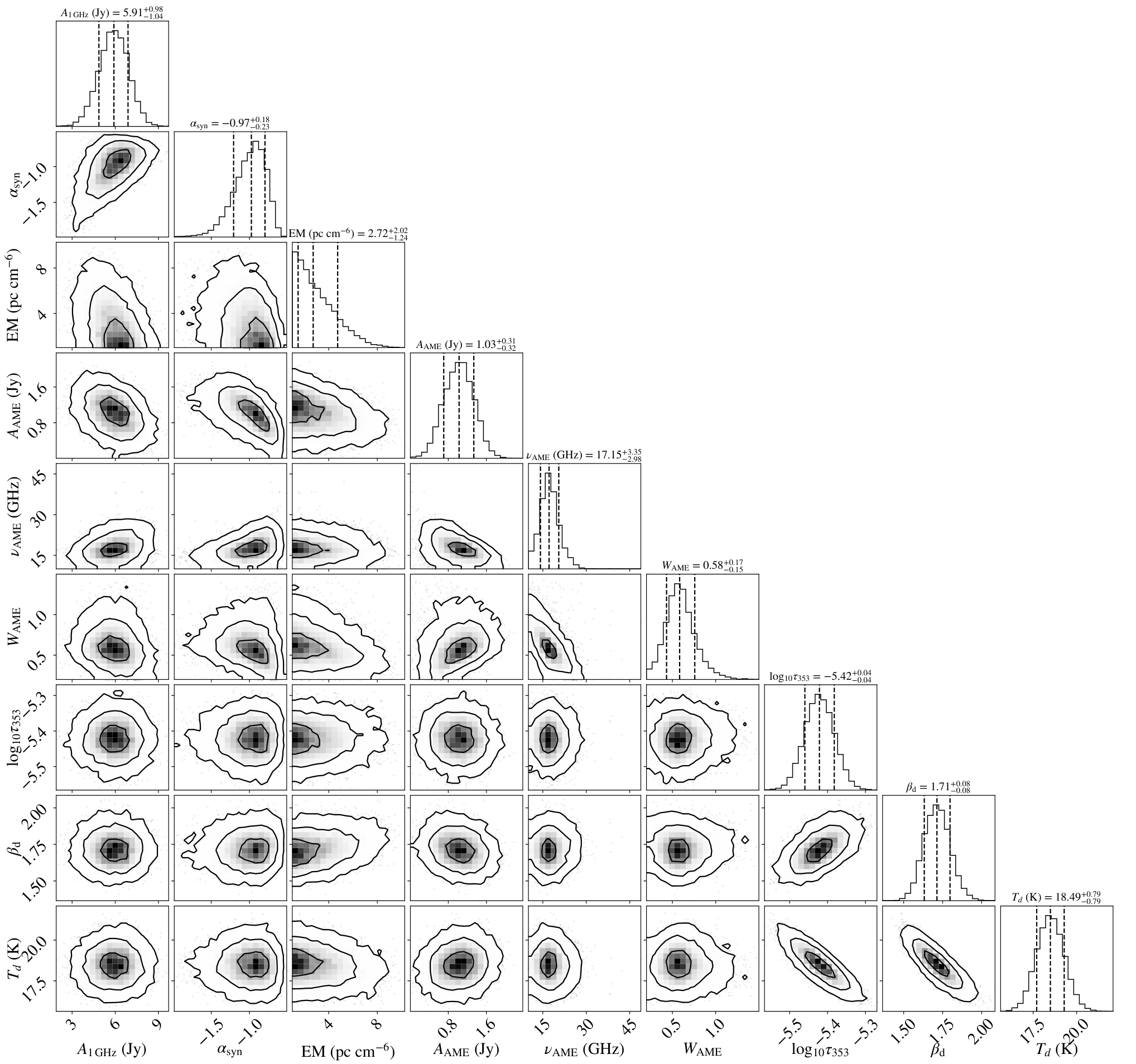
We recover the AME peak flux density parameter, , in M31 with a significance, as can be seen in Table 4 and Fig. 4: . At 25 GHz, we estimate the AME flux density to be , 1.7 below the value of Jy quoted by 5. The reason for this difference could be that our measured flux densities between 10 and 60 GHz (where AME is expected to be most important) are lower than those from 5, probably due to differences in the filtering of the ancillary data together with the different choices for the CMB map (5 used SMICA while we are using NILC, as further discussed in Sections 3.5 and 5.1). For example, our photometry estimate for Planck 28.4 GHz band is 74% than that from 5: correcting for that factor, our estimates at 25 GHz would increase to , closer to those from 5. The corner plot showing the parameter posteriors used to build the previous SED is shown in Fig. 5.
Our fitted synchrotron spectral index, is consistent with those obtained by Berkhuijsen et al. 2003, , and Planck Collaboration et al. 2015b, . It is also consistent with the value obtained by 5, , owing to large uncertainty in this parameter due to unresolved parameter degeneracies. This is because of the lack of data with good calibration uncertainties below 10 GHz. It is worth noting that, except for the thermal dust spectral index, the differences between our best-fit parameters and those of 5 are always within the level. The study of 5 benefitted from the addition of the SRT data point at 6.6 GHz, which is critical to alleviate the degeneracy between the synchrotron and free–free components. The value of our fit at 6.6 GHz is not too different from the one quoted in the analysis of 5: our flux density estimate value is Jy compared to Jy from 5. The two are only away.
Degeneracy with synchrotron emission prevents a precise determination of the level of free–free emission from our compoment-separation analysis. Actually, Fig. 5 clearly shows that the 1D posterior of EM is consistent with a non-detection of free-free emission, and an upper limit would probably be more appropriate. The 68% upper limit on the free-free flux density at 1 GHz derived from this posterior is 0.52 Jy. This is consistent with the expected value derived from the H emission. By integration on the map of Finkbeiner 2003 with the aperture and background annulus described in Section 3.2, and using the formalism explained in Dickinson et al. 2003, we derive an expected free–free flux density at 1 GHz of Jy. Due to absorption of H emission this value might be regarded as a lower limit. Absorption correction suffers from important uncertainties, related for instance with the way absorption measured at other wavelengths is translated into H absorption. Using the formalism described in Dickinson et al. 2003 and the reddening map derived by the Planck collaboration (Planck Collaboration et al. 2014b) we get Jy. If we instead use the reddening map, also derived by the Planck collaboration (Planck Collaboration et al. 2016a) we get Jy. These values are both consistent with our derived upper limit.
Another common way of estimating free-free emission relies on measurements of the star formation rate (SFR). Ford et al. 2013 measured /yr from UV and 24-micron data. Equation 6 of Murphy et al. 2012 provides a relation between SFR and spectral luminosity. Using this equation and assuming an average electron temperature K (typical value from our Galaxy) we get W/Hz at 1 GHz. From this, and using a distance to M31 of pc (McConnachie et al. 2005) we get a flux density at 1 GHz of Jy, a value that is roughly consistent with our derived upper limit (we have intentionally omitted the statistical error in this estimate as systematic errors associated with the scaling relations used are expected to be larger).
Thus, given that the estimate for the amplitude of free–free is consistent with zero, we repeated our analysis without taking this component into account. The absence of a free–free contribution is compensated by a slightly wider AME component: now, as compared to when free--free was considered.99 9 In fact, we can see in the corner plot (Fig. 5) that the free–free amplitude and are slightly anticorrelated. Large values of imply wide AME distributions that could resemble power-law distributions similar to free–free between 10 and 60 GHz, where AME is most important. However, most AME theory models (Ali-Haïmoud et al. 2009; Silsbee et al. 2011, SPDUST,) expect values for smaller than 0.6. Previous studies have resolved this issue by adding a second AME component (e.g. Planck Collaboration et al. 2016b). However, in the case of the integrated emission from a galaxy like ours, we expect a large number of AME emitting regions with different spectral parameters within our aperture, leading to a broadening of the integrated AME distribution. We tried to fit a second AME component, but found that the MCMC chains stopped converging and the parameters defining this new component were not properly constrained. In conclusion, we decided to use as the default model in this analysis the one with free–free emission, even though its value is slightly higher than the value when no free–free is considered ( vs. , being systematically smaller than 1 most probably owing to an overestimation of the photometry uncertainties). This decision is based on the fact that we know, from different kinds of observational evidence (e.g. the presence of star formation or H emission), that free–free emission originating in M31 must exist.
4.1 Statistical evaluation of the presence of AME in M31
We repeated the analysis without the AME component to ensure that AME in M31 could not be mistaken for free–free emission. The value obtained in that case is at least a factor 2.5 worse than any of the two other scenarios where an AME component is introduced (Table 4). values are computed using the median values from the distributions of the parameter posteriors shown in Fig. 5. These median values are those quoted in the table. The worst fit is the one for which no AME component is considered.
We used the Akaike information criterion (Akaike 1974, AIC,) and the Bayesian information criterion (Schwarz 1978, BIC,) to compare the goodness of the fits with and without AME. This was done in order to account for the non-Gaussianity of the likelihood, mostly due to the presence of non-linear parameters in the SED fitting (e.g. the synchrotron spectral index). AIC and BIC are computed as follows:
| (8) |
where stands for the number of fitted parameters, while is the number of data points introduced in the fit. is the maximum log-likelihood value computed within the MCMC, as explained in Section 3.3 and Eq. 5. Larger differences on the AIC or BIC estimates from two models will imply a heavier preference of the data for the model with the lowest value. The main difference between the two is that the BIC penalizes the addition of parameters more heavily than the AIC. We compare the case with all the components and the case without AME, as we previously explained that the case with no free–free component is not physical:
According to the AIC, the relative likelihood of the model without an AME component compared to the model with all components considered is:
and the model with AME is strongly preferred. When using the BIC, we found the relative likelihood of the model without AME to be:
over a factor 4 larger. This is consistent with BIC penalizing the larger number of parameters considered in the case with all components, compared to that without AME. However, the model without AME is still below 0.01 times as probable as that with AME, pointing to a strong preference for the latter.
| Case 1 (all components) | Case 2 (no AME) | Case 3 (no free-free) | From Battistelli et al. 2019 | |
| (Jy) | ||||
| EM (pc / cm6) | - | - | ||
| [Jy] | - | - | ||
| [GHz] | - | - | ||
| - | - | |||
| - | ||||
| [K] | ||||
| (Jy) | - | |||
| @ 25 GHz (Jy) | - | |||
| (Jy) | ||||
| 0.61 | 1.51 | 0.39 | 0.36 |
4.2 The global properties of M31 compared to the Milky Way
As pointed out in Section 1, M31 is the galaxy most similar to the MW in the Local Group. Therefore, it is straightforward to compare the properties between the two, especially for AME, which is the main focus of our study. First, we computed the AME emissivity for M31 as done in Fernández-Torreiro et al. 2023, i.e. as the ratio between the AME intensity at 28.4 GHz (in temperature units) and the dust intensity at 100 from the fit:
| (9) |
This ratio is intended to cancel the dependence on the column density, present in both AME and thermal dust emission, thus allowing us to compare regions with extremely different morphologies. As pointed out by Tibbs et al. 2012 this cancellation may not be perfect as this calculation of the AME emissivity is sensitive to the dust temperature. However thanks to the similarity between dust temperatures in M31 and in the MW this should not be a problem in our comparison.
Differences between 5 and this work on dust parameters arise because of the different surveys used (Herschel and COBE-DIRBE, respectively). We find K/(MJy/sr), and compare it to the results for the MW both from the Planck collaboration (Planck Collaboration et al. 2015a) and also Section 4.2 of Fernández-Torreiro et al. 2023. Planck Collaboration et al. 2015a quoted a K/(MJy/sr) value1010 10 There seems to be a typo on this Planck paper, as in Section 7.3 the units for the emissivity are quoted as mK/(MJy/sr) instead of K/(MJy/sr). for the MW, fully consistent with our M31 result, while Fernández-Torreiro et al. 2023 returns K/(MJy/sr), which is a lower value, but still consistent because of the large uncertainties1111 11 This estimate increases when only those pixels with strong AME detections are used, up to K/(MJy/sr). Both values are lower than those previously found in several other works (see e.g. Table 3 of Dickinson et al. 2018), but the AME emissivity can show large variations (Davies et al. 2006 found variations as large as a factor 2, for example). Those variations would probably be embedded within the integrated spectrum of the galaxy, effectively decreasing the AME emissivity value with respect to that found in compact sources.
When computing the AME fraction at 28.4 GHz we find . This is slightly greater than the values obtained by Fernández-Torreiro et al. 2023 and Planck Collaboration et al. 2015a, and respectively, although it is consistent to within , owing to the greater uncertainty in the M31 estimate. Finally, when focusing on the synchrotron spectral index, we find consistent estimates between M31 and the MW of and (Fernández-Torreiro et al. 2023) respectively.
4.3 QUIJOTE-MFI M31 upper limits on polarization
As explained in Section 2.1, the M31 field has the best sensitivity values (shown in Table 2) of all the fields studied by QUIJOTE-MFI so far, being slightly better than those from the Haze (Guidi et al. 2023) and W49, W51 and IC443 (Tramonte et al. 2023) fields. This is because of the long integration times invested in those regions. Stokes and maps of the M31 field are displayed in Fig. 7.

Given the lack of any detectable polarized signal towards M31 on the QUIJOTE-MFI maps, we derived upper limits on its global polarized flux density. Using the same photometric approach and apertures as for intensity (Section 3.2), the measured Stokes and parameters are Jy and Jy at 11 GHz, and Jy and Jy at 13 GHz. Except for the value at 13 GHz showing a marginal detection, they are statistically consistent with zero. Taking the measured values as upper limits, the noise debiased1212 12 Computed following Vaillancourt 2006 and Rubiño-Martín et al. 2012. polarized intensity estimates, , are Jy and Jy, respectively at 11 and 13 GHz for a 95% confidence limit (C.L.)). The flux density estimates at 11 and 13 GHz are Jy and Jy (after subtracting both the point sources and the CMB, as shown in Table 1), so the polarization fractions for the integrated M31 flux density are below and , respectively, for a 95% C.L. Considering the AME contribution to the total flux in intensity, the polarization fraction upper limits derived from this analysis are at 11 GHz and at 13 GHz. Although this upper limit is an order of magnitude greater than the most stringent ones obtained from the analysis of AME sources in the MW (Génova-Santos et al. 2017; Tramonte et al. 2023; González-González et al. 2023, e.g., ), this is the first time that a limit on the AME polarization has been obtained for an extragalactic object. It must be noted though that a potential underlying AME polarization in M31 in small angular scales may be largely smeared out in our aperture due to mixing of different polarization orientations. This would also be the case for a possible polarization of the synchrotron emission, that in specific regions of M31 is known to reach values of (Berkhuijsen et al. 2003). In any case, owing to the sensitivity of our polarization data, and to the uncertainty in the determination of the integrated total-intensity flux density of the synchrotron emission, our derived constraints on the global synchrotron polarization fraction are above this level.
5 Robustness tests
5.1 Impact of the selected CMB map on the AME amplitude
As first mentioned in Section 3.5, different CMB maps yield different integrated measurements on the M31 aperture. These affect the photometry flux densities computed to build the SED as in Eq. 2. We mentioned that the measurement from SMICA is the largest of the four maps, which implies a decrease in M31 flux densities at microwave frequencies (). This produces a steeper spectrum in this frequency range, and thus an AME component is preferred over free-free or synchrotron. In the opposite scenario, the measurement from COMMANDER is lower, thus flattening the SED at those frequencies and decreasing AME amplitude.
We ran the same analysis as in Section 4 after using SMICA and COMMANDER instead of NILC to subtract the CMB anisotropies. AME amplitude increases to when the SMICA map is used, and decreases to when using COMMANDER. Thus, the AME significance changes from to depending on the choice of the CMB map. Besides, the higher value when subtracting the signal from SMICA implies a lower free-free amplitude and steeper synchrotron index. In the COMMANDER case the situation is the opposite: the decrease implies a larger free-free component and a flatter synchrotron spectrum. Because of the differences between the two cases, we decided to use the NILC CMB map, which returns a significance instead, as a trade-off scenario.
5.2 QUIJOTE-MFI role in the fitting
We repeated the former analyses without taking into account the data from QUIJOTE-MFI. In this way, we can assess its constraining power. We show the results in Table 5 and the corresponding SED for the general (all emission components considered) case in Fig. 8. The significance of the measurement of is slightly reduced to when the QUIJOTE-MFI data are not used. The AME amplitude, , remains the same: it is now Jy compared to the previous value of Jy. However, we find that the posterior is now not constrained at lower values. This implies an increase on its uncertainty, so , compared to when using QUIJOTE-MFI data. This is directly related to the absence of data in that frequency range (5–20 GHz). The larger uncertainty also implies larger differences between the preferred models when using the max-likelihood solution or that from the 1D distributions median values. The change is not as important for the AME width, , as it is now compared to the previous value of . Therefore, QUIJOTE-MFI data addition significantly reduces (almost by a factor 2) the uncertainty of the parameter. Finally, we can see that the model providing the worst fit to the data is again the one trying to account for all emission with just synchrotron and free–free components and no AME component.
| Case 1 (all components) | Case 2 (no AME) | Case 3 (no free-free) | From Battistelli et al. 2019 | |
| (Jy) | ||||
| EM (pc / cm6) | - | - | ||
| [Jy] | - | - | ||
| [GHz] | - | - | ||
| - | - | |||
| - | ||||
| [K] | ||||
| (Jy) | - | |||
| @ 25 GHz (Jy) | - | |||
| (Jy) | ||||
| 0.62 | 1.53 | 0.39 | 0.36 |
5.3 Source subtraction effect
We repeated our analysis of the maps with no point source subtraction applied, but keeping QUIJOTE-MFI data. This was done in order to assess the impact of this subtraction on the level of AME. Results for this case are shown in Table 6. The general case (all emission components considered) is also shown in the bottom panel of Fig. 8. As it was the case when discarding QUIJOTE-MFI data, the uncertainties on the AME parameters increased, thus reducing the significance for those parameters. There are slight changes in some parameters. In particular, the synchrotron becomes flatter, and as a result there is more synchrotron at microwave frequencies. The level of free-free is higher: as a consequence from both changes, the AME amplitude is lower. Therefore, the significance of is now lower too, down to . The and values do not change significantly with respect to the main case presented in Section 4: GHz and , respectively, compared to GHz and . The changes of all parameters are always within .
| Case 1 (all components) | Case 2 (no AME) | Case 3 (no free-free) | From Battistelli et al. 2019 | |
| (Jy) | ||||
| EM (pc / cm6) | - | - | ||
| [Jy] | - | - | ||
| [GHz] | - | - | ||
| - | - | |||
| - | ||||
| [K] | ||||
| (Jy) | - | |||
| @ 25 GHz (Jy) | - | |||
| (Jy) | ||||
| 0.46 | 0.95 | 0.36 | 0.36 |
5.4 Impact from changes in the background aperture
Finally, we repeated the analysis using the same elliptical aperture used in Harper et al. 2023, which is also similar to the one introduced in Planck Collaboration et al. 2015b. These regions have major semiaxes equal to 100, 110 and 154 arcminutes, the last two being the inner and outer radii of the ring enclosing the background region. The minor-to-major ratio is 0.7 for all three, with an east-to-north position angle equal to . When comparing with Planck Collaboration et al. 2015b, we are introducing the MFI data and subtracting the CMB using NILC as a template (plus adding an uncertainty term to account for the dispersion in the values of the CMB templates, as explained in Section 3.5). Our main difference with Harper et al. 2023 is the addition of the QUIJOTE-MFI raster data presented in Section 2.1, while we lack the point from C-BASS at 4.76 GHz. That paper also used SMICA instead of NILC to account for CMB anisotropies: we found that SMICA systematically returned higher estimates for the AME than the rest of maps (following the discussions in Sections 3.5 and 5.1). We are also not keeping the point source subtraction because of the paucity of objects in Fatigoni et al. 2021 outside the SRT M31 field. Results are shown in Table 7 (where we show the case from Harper et al. 2023 with no subtraction of sources, as it is the most similar one to our analysis) and the corresponding SEDs in Fig. 9. We recover an AME estimate with reduced significance () only: Jy. Note though that the differences between our parameters and those of Harper et al. 2023 are always below the level.
We find that the result in our study for the synchrotron index, , is consistent with those of Berkhuijsen et al. 2003 and Planck Collaboration et al. 2015b ( vs. and respectively), but steeper than that of Harper et al. 2023 (). The synchrotron amplitude, is consistent between this study and Planck Collaboration et al. 2015b and Harper et al. 2023: Jy vs. and , respectively. Our free–free estimate is larger, although consistent with a non detection to within 2 too: pc cm-6 vs. pc cm-6 and pc cm-6. We get a similar consistency in the AME amplitude with Planck Collaboration et al. 2015b ( vs. Jy), and the value from Harper et al. 2023 ( Jy) is within . The AME peak frequency value increased slightly from Section 4 to GHz, while AME width decreased to . Harper et al. 2023 found a higher value for , GHz. However, one must take into account that our model includes an additional free varying parameter driving the width of the AME distribution. On the other hand, both Planck Collaboration et al. 2015b and Harper et al. 2023 fixed this value by assuming that the AME was fully explained by a single template model (WIM and WNM templates from SPDUST -Ali-Haïmoud et al. 2009; Silsbee et al. 2011-, respectively). Our approach would be more similar to a galaxy hosting multiple AME regions with different spectral dependencies.
Finally, the AME emissivity in this case can be also computed: we find K/, much higher than the one obtained by Harper et al. 2023. The estimate is lower than that from Section 4.2, being K MJy-1 sr, although within 1, because of the large uncertainties.
When evaluating our fit at C-BASS nominal frequency, 4.76 GHz, we find Jy, the large dispersion being consistent with the lack of data between 2–10 GHz. This difference with the value quoted in Harper et al. 2023 ( Jy) is between the differences for 1.42 GHz and QUIJOTE-MFI surveys (1.5 Jy and 0.55 Jy respectively). It is noticeable in Fig. 9 that the C-BASS measurement falls well within the uncertaintiy of our fitted model. Finally, it is worth noting that C-BASS and QUIJOTE are calibrated to different calibration scales. As explained in Harper et al. 2023 C-BASS data uses the model for Tau A of Weiland et al. 2011. On the contrary, as explained in Rubiño-Martín et al. 2023, QUIJOTE data are calibrated to an updated model that is based on the same data used by Weiland et al. 2011, but including some improvements and the addition of Tau A flux densities from Planck data. Evaluation of the C-BASS model at 4.76 GHz for epoch 2014.4 (C-BASS reference epoch, as observations took place between July 2013 and March 2015) yields a value that is higher than the prediction from the QUIJOTE model. Therefore rescaling the C-BASS point to the QUIJOTE model results in 3.89 Jy, an even better consistency with the fitted models shown in Fig. 9.
| Case 1 (all components) | Case 2 (no AME) | Case 3 (no free-free) | Planck Collaboration et al. 2015b | Harper et al. 2023 | |
| (Jy) | |||||
| EM (pc / cm6) | - | ||||
| [Jy] | - | - | - | ||
| [GHz] | - | - | |||
| - | - | ||||
| [K] | |||||
| (Jy) | - | - | - | ||
| @ 25 GHz (Jy) | - | ||||
| (Jy) | - | ||||
| 0.77 | 1.12 | 0.71 | 1.1 | 2.6 |
6 Conclusions
In this study we used new data from the QUIJOTE-MFI experiment at 10–20 GHz to study the Andromeda Galaxy (M31). We built the integrated SED in intensity of M31 between 0.408 and 3000 GHz, and performed a component separation analysis after subtracting the emission from CMB anisotropies and point sources in the region present in the Fatigoni et al. 2021 catalogue. We measure the AME amplitude with a significance of in the integrated SED of M31, independently of the previous 5 detection. Moreover, our fitted model is consistent with the 6.6 GHz measurement provided by that study. The addition of QUIJOTE-MFI data improves the definition of AME spectral parameters: its peak frequency, GHz, and width, . is low for most theoretical models but is consistent with most recent studies pointing to being below 21 GHz (Harper et al. 2022; Fernández-Torreiro et al. 2023, e.g.). However, is slightly greater than expected from theoretical models, but again consistent with recent studies (Poidevin et al. 2023; Fernández-Torreiro et al. 2023, e.g.). This can be explained by the probable large number of AME regions within M31 with different and values, which naturally broaden the distribution of the integrated measurement. Nevertheless, the significance of the AME detection is not as dependent on the QUIJOTE-MFI data addition as on the subtraction of point sources. The significance of the measurement of is still greater than 3 () when discarding the QUIJOTE-MFI data, but this significance falls below 3 () when no point source subtraction is applied. The significance also falls below when the COMMANDER map is used to subtract the CMB anisotropies instead of NILC or SMICA, highlighting the importance of the choice of the CMB map. When studying the AME emissivity in M31, we found K/(MJy/sr) compared to the K/(MJy/sr) estimate obtained by Fernández-Torreiro et al. 2023 for the Milky Way, pointing to a similar AME behaviour in both.
We also provided a similar comparison to Harper et al. 2023, who recently measured AME in M31 again, although with much lower amplitude than the previous studies of 5 and of Planck Collaboration et al. 2015b. This difference is driven mainly by the lower flux density derived from SRT data in 5 as compared with the C-BASS value of Harper et al. 2023. However, the two works also show important differences in their data analysis processes. Especially, the different apertures used to perform aperture photometry are of extremely importance. We find consistent results with both when replicating each of the methodologies, while being independent from them - i.e. not using their data. The AME emissivity estimate from Harper et al. 2023 is off by a factor larger than 20 when compared with previous measurements (Planck Collaboration et al. 2015a; Harper et al. 2022; Fernández-Torreiro et al. 2023). When replicating the conditions from Harper et al. 2023, we obtain an AME emissivity estimate K/(MJy/sr), lower than the previous value of K/(MJy/sr) probably due to the larger importance of the outskirts of M31. This probably explains why this value is also lower than the estimate for the MW: when observing the MW from its inside, we are not sensitive to these outer regions. This emissivity estimate is equal to K/ in units, more in line with previous measurements (Davies et al. 2006; Planck Collaboration et al. 2015a; Planck Collaboration et al. 2016c; Hensley & Draine 2017; Harper et al. 2022; Fernández-Torreiro et al. 2023) than the one from Harper et al. 2023.
M31 remains the only detection to date of AME in the integrated spectrum of an external galaxy. We have also provided upper limits for the polarization of this AME component. Although these limits are large when compared with those from brighter AME sources (mostly within our Galaxy), this is the first time that such upper limits have been computed for an extragalactic object. The results of this work encourage the reproduction of this kind of of measurement for galaxies with different sets of properties throughout the lifetime of the Universe.
Acknowledgements
We thank the staff of the Teide Observatory for invaluable assistance in the commissioning and operation of QUIJOTE. The QUIJOTE experiment is being developed by the Instituto de Astrofisica de Canarias (IAC), the Instituto de Fisica de Cantabria (IFCA), and the Universities of Cantabria, Manchester and Cambridge. Partial financial support was provided by the Spanish Ministry of Science and Innovation under the projects AYA2007-68058-C03-01, AYA2007-68058-C03-02, AYA2010-21766-C03-01, AYA2010-21766-C03-02, AYA2014-60438-P, ESP2015-70646-C2-1-R, AYA2017-84185-P, ESP2017-83921-C2-1-R, PID2019-110610RB-C21, PID2020-120514GB-I00, IACA13-3E-2336, IACA15-BE-3707, EQC2018-004918-P, the Severo Ochoa Programs SEV-2015-0548 and CEX2019-000920-S, the Maria de Maeztu Program MDM-2017-0765 and by the Consolider-Ingenio project CSD2010-00064 (EPI: Exploring the Physics of Inflation). We acknowledge support from the ACIISI, Consejeria de Economia, Conocimiento y Empleo del Gobierno de Canarias and the European Regional Development Fund (ERDF) under grant with reference ProID2020010108. This project has received funding from the European Union’s Horizon 2020 research and innovation program under grant agreement number 687312 (RADIOFOREGROUNDS). We thank the anonymous referee whose comments helped to improve this work. MFT acknowledges support from from the Agencia Estatal de Investigación (AEI) of the Ministerio de Ciencia, Innovación y Universidades (MCIU) and the European Social Fund (ESF) under grant with reference PRE-C-2018-0067. C.A-T acknowledges support from the Millennium Nucleus on Young Exoplanets and their Moons (YEMS). FP acknowledges support from the Agencia Canaria de Investigación, Innovación y Sociedad de la Información (ACIISI) under the European FEDER (FONDO EUROPEO DE DESARROLLO REGIONAL) de Canarias 2014-2020 grant No. PROID2021010078. We acknowledge the use of data provided by the Centre d’Analyse de Données Etendues (CADE), a service of IRAP-UPS/CNRS (http://cade.irap.omp.eu, Paradis et al. 2012). This research has made use of the SIMBAD database, operated at CDS, Strasbourg, France (Wenger et al. 2000). Some of the results in this paper have been derived using the healpy and HEALPix packages (Górski et al. 2005; Zonca et al. 2019). We have also used scipy (Virtanen et al. 2020), emcee (Foreman-Mackey et al. 2013), numpy (Harris et al. 2020), matplotlib (Hunter 2007), corner (Foreman-Mackey 2016) and astropy (Astropy Collaboration et al. 2013; Astropy Collaboration et al. 2018) python packages.
Data availability
The QUIJOTE raster scan data used in this paper are property of the QUIJOTE Collaboration and can only be shared on request to the corresponding authors. All M31 fits are available upon reques to the QUIJOTE collaboration. QUIJOTE-MFI Wide Survey data is available in the QUIJOTE collaboration webpage (https://research.iac.es/proyecto/quijote).
References
- Akaike (1974) Akaike H., 1974, IEEE Transactions on Automatic Control, 19, 716
- Ali-Haïmoud et al. (2009) Ali-Haïmoud Y., Hirata C. M., Dickinson C., 2009, MNRAS, 395, 1055
- Astropy Collaboration et al. (2013) Astropy Collaboration et al., 2013, A&A, 558, A33
- Astropy Collaboration et al. (2018) Astropy Collaboration et al., 2018, AJ, 156, 123
- Battistelli et al. (2019) Battistelli E. S., et al., 2019, ApJ, 877, L31
- Bennett et al. (2013) Bennett C. L., et al., 2013, ApJS, 208, 20
- Berkhuijsen (1972) Berkhuijsen E. M., 1972, A&AS, 5, 263
- Berkhuijsen et al. (2003) Berkhuijsen E. M., Beck R., Hoernes P., 2003, A&A, 398, 937
- Bianchi et al. (2022) Bianchi S., et al., 2022, A&A, 658, L8
- Cepeda-Arroita et al. (2021) Cepeda-Arroita R., et al., 2021, MNRAS, 503, 2927
- Davies et al. (2006) Davies R. D., Dickinson C., Banday A. J., Jaffe T. R., Górski K. M., Davis R. J., 2006, MNRAS, 370, 1125
- Dickinson et al. (2003) Dickinson C., Davies R. D., Davis R. J., 2003, MNRAS, 341, 369
- Dickinson et al. (2011) Dickinson C., Peel M., Vidal M., 2011, MNRAS, 418, L35
- Dickinson et al. (2018) Dickinson C., et al., 2018, New Astron. Rev., 80, 1
- Draine & Lazarian (1998a) Draine B. T., Lazarian A., 1998a, ApJ, 494, L19
- Draine & Lazarian (1998b) Draine B. T., Lazarian A., 1998b, ApJ, 508, 157
- Fatigoni et al. (2021) Fatigoni S., et al., 2021, A&A, 651, A98
- Fernández-Torreiro et al. (2023) Fernández-Torreiro M., et al., 2023, MNRAS,
- Finkbeiner (2003) Finkbeiner D. P., 2003, ApJS, 146, 407
- Ford et al. (2013) Ford G. P., et al., 2013, ApJ, 769, 55
- Foreman-Mackey (2016) Foreman-Mackey D., 2016, Journal of Open Source Software, 1, 24
- Foreman-Mackey et al. (2013) Foreman-Mackey D., Hogg D. W., Lang D., Goodman J., 2013, PASP, 125, 306
- Fritz et al. (2012) Fritz J., et al., 2012, A&A, 546, A34
- Génova-Santos et al. (2015) Génova-Santos R., et al., 2015, MNRAS, 452, 4169
- Génova-Santos et al. (2017) Génova-Santos R., et al., 2017, MNRAS, 464, 4107
- González-González et al. (2023) González-González R., et al., 2023, MNRAS, in prep.
- Goodwin et al. (1998) Goodwin S. P., Gribbin J., Hendry M. A., 1998, The Observatory, 118, 201
- Górski et al. (2005) Górski K. M., Hivon E., Banday A. J., Wand elt B. D., Hansen F. K., Reinecke M., Bartelmann M., 2005, ApJ, 622, 759
- Guidi et al. (2021) Guidi F., et al., 2021, MNRAS, 507, 3707
- Guidi et al. (2023) Guidi F., et al., 2023, MNRAS, 519, 3460
- Harper et al. (2022) Harper S. E., et al., 2022, MNRAS, 513, 5900
- Harper et al. (2023) Harper S. E., et al., 2023, arXiv e-prints, p. arXiv:2304.03875
- Harris et al. (2020) Harris C. R., et al., 2020, Nature, 585, 357
- Haslam et al. (1982) Haslam C. G. T., Salter C. J., Stoffel H., Wilson W. E., 1982, A&AS, 47, 1
- Hauser et al. (1998) Hauser M. G., et al., 1998, ApJ, 508, 25
- Healey et al. (2007) Healey S. E., Romani R. W., Taylor G. B., Sadler E. M., Ricci R., Murphy T., Ulvestad J. S., Winn J. N., 2007, ApJS, 171, 61
- Hensley & Draine (2017) Hensley B. S., Draine B. T., 2017, ApJ, 836, 179
- Hensley et al. (2015) Hensley B., Murphy E., Staguhn J., 2015, MNRAS, 449, 809
- Herman et al. (2022) Herman D., et al., 2022, arXiv e-prints, p. arXiv:2201.03530
- Hunter (2007) Hunter J. D., 2007, Computing in Science & Engineering, 9, 90
- Kogut et al. (1996) Kogut A., Banday A. J., Bennett C. L., Gorski K. M., Hinshaw G., Smoot G. F., Wright E. I., 1996, ApJ, 464, L5
- Leitch et al. (1997) Leitch E. M., Readhead A. C. S., Pearson T. J., Myers S. T., 1997, ApJ, 486, L23
- López-Caraballo et al. (2011) López-Caraballo C. H., Rubiño-Martín J. A., Rebolo R., Génova-Santos R., 2011, ApJ, 729, 25
- Lopez-Caraballo et al. (2023) Lopez-Caraballo C. H., et al., 2023, MNRAS, in prep.
- Macellari et al. (2011) Macellari N., Pierpaoli E., Dickinson C., Vaillancourt J. E., 2011, MNRAS, 418, 888
- McConnachie et al. (2005) McConnachie A. W., Irwin M. J., Ferguson A. M. N., Ibata R. A., Lewis G. F., Tanvir N., 2005, MNRAS, 356, 979
- Murphy et al. (2010) Murphy E. J., et al., 2010, ApJ, 709, L108
- Murphy et al. (2012) Murphy E. J., et al., 2012, ApJ, 761, 97
- Murphy et al. (2018) Murphy E. J., Linden S. T., Dong D., Hensley B. S., Momjian E., Helou G., Evans A. S., 2018, ApJ, 862, 20
- Paradis et al. (2012) Paradis D., Dobashi K., Shimoikura T., Kawamura A., Onishi T., Fukui Y., Bernard J. P., 2012, A&A, 543, A103
- Peel et al. (2011) Peel M. W., Dickinson C., Davies R. D., Clements D. L., Beswick R. J., 2011, MNRAS, 416, L99
- Peel et al. (2022) Peel M. W., Genova-Santos R., Dickinson C., Leahy J. P., López-Caraballo C., Fernández-Torreiro M., Rubiño-Martín J. A., Spencer L. D., 2022, Research Notes of the American Astronomical Society, 6, 252
- Planck Collaboration et al. (2014a) Planck Collaboration et al., 2014a, A&A, 565, A103
- Planck Collaboration et al. (2014b) Planck Collaboration et al., 2014b, A&A, 571, A11
- Planck Collaboration et al. (2015a) Planck Collaboration et al., 2015a, A&A, 580, A13
- Planck Collaboration et al. (2015b) Planck Collaboration et al., 2015b, A&A, 582, A28
- Planck Collaboration et al. (2016a) Planck Collaboration et al., 2016a, A&A, 586, A132
- Planck Collaboration et al. (2016b) Planck Collaboration et al., 2016b, A&A, 594, A10
- Planck Collaboration et al. (2016c) Planck Collaboration et al., 2016c, A&A, 594, A25
- Planck Collaboration et al. (2020a) Planck Collaboration et al., 2020a, A&A, 641, A1
- Planck Collaboration et al. (2020b) Planck Collaboration et al., 2020b, A&A, 641, A4
- Poidevin et al. (2019) Poidevin F., et al., 2019, MNRAS, 486, 462
- Poidevin et al. (2023) Poidevin F., et al., 2023, MNRAS, 519, 3481
- Reich (1982) Reich W., 1982, A&AS, 48, 219
- Reich & Reich (1988) Reich P., Reich W., 1988, A&AS, 74, 7
- Reich et al. (2001) Reich P., Testori J. C., Reich W., 2001, A&A, 376, 861
- Remazeilles et al. (2015) Remazeilles M., Dickinson C., Banday A. J., Bigot-Sazy M. A., Ghosh T., 2015, MNRAS, 451, 4311
- Richards et al. (2011) Richards J. L., et al., 2011, ApJS, 194, 29
- Rubiño-Martín et al. (2010) Rubiño-Martín J. A., et al., 2010, Astrophysics and Space Science Proceedings, 14, 127
- Rubiño-Martín et al. (2012) Rubiño-Martín J. A., López-Caraballo C. H., Génova-Santos R., Rebolo R., 2012, Advances in Astronomy, 2012, 351836
- Rubiño-Martín et al. (2023) Rubiño-Martín J. A., et al., 2023, MNRAS, 519, 3383
- Ruiz-Granados et al. (2023) Ruiz-Granados B., et al., 2023, MNRAS, in prep.
- Rys & Machalski (1990) Rys S., Machalski J., 1990, A&A, 236, 15
- Schwarz (1978) Schwarz G., 1978, Annals of Statistics, 6, 461
- Silsbee et al. (2011) Silsbee K., Ali-Haïmoud Y., Hirata C. M., 2011, MNRAS, 411, 2750
- Stevenson (2014) Stevenson M. A., 2014, ApJ, 781, 113
- Tibbs et al. (2012) Tibbs C. T., Paladini R., Dickinson C., 2012, Advances in Astronomy, 2012, 124931
- Tibbs et al. (2018) Tibbs C. T., Israel F. P., Laureijs R. J., Tauber J. A., Partridge B., Peel M. W., Fauvet L., 2018, MNRAS, 477, 4968
- Tramonte et al. (2023) Tramonte D., et al., 2023, MNRAS, 519, 3432
- Vaillancourt (2006) Vaillancourt J. E., 2006, PASP, 118, 1340
- Virtanen et al. (2020) Virtanen P., et al., 2020, Nature Methods, 17, 261
- Watson et al. (2005) Watson R. A., Rebolo R., Rubiño-Martín J. A., Hildebrandt S., Gutiérrez C. M., Fernández-Cerezo S., Hoyland R. J., Battistelli E. S., 2005, ApJ, 624, L89
- Weiland et al. (2011) Weiland J. L., et al., 2011, ApJS, 192, 19
- Wenger et al. (2000) Wenger M., et al., 2000, A&AS, 143, 9
- Zonca et al. (2019) Zonca A., Singer L., Lenz D., Reinecke M., Rosset C., Hivon E., Gorski K., 2019, Journal of Open Source Software, 4, 1298
- de Vaucouleurs et al. (1991) de Vaucouleurs G., de Vaucouleurs A., Corwin Herold G. J., Buta R. J., Paturel G., Fouque P., 1991, Third Reference Catalogue of Bright Galaxies