跳到论文正文
W Papers独立论文阅读器 arXiv:2305.08427 论文正文 计算阅读时间 · 0%
引用这篇论文根据当前论文元数据生成,正式投稿前建议核对。


License: arXiv.org perpetual non-exclusive license
arXiv:2305.08427v1 [math.AP] 15 May 2023

Peculiarities of Space Dependent Conservation Laws: Inverse Design and Asymptotics

Rinaldo M. Colombo Affiliation: Unità INdAM & Dipartimento di Ingegneria dell’Informazione, Università di Brescia E-mail: rinaldo.colombo@unibs.it    Vincent Perrollaz and Abraham Sylla
Abstract

Recently, results regarding the Inverse Design problem for Conservation Laws and Hamilton-Jacobi equations with xx-dependent convex fluxes were obtained in CPS2022; CPS2023. More precisely, characterizations of attainable sets and the set of initial data evolving at a prescribed time into a prescribed profile were obtained. Here, we present an explicit example that underlines deep differences between the xx-dependent and xx-independent cases. Moreover, we add a detailed analysis of the time asymptotic solution of this example, again underlining differences with the xx-independent case.

1 Introduction

Consider the scalar one dimensional conservation law

{∂tu+∂x(H⁡(x,u))=0(t,x)∈]0,+∞[×ℝu​(0,x)=uo​(x)x∈ℝ.\left\{\begin{array}[]{l@{\qquad}r@{\,}c@{\,}l}\partial_{t}u+\partial_{x}(H(x,u))=0&(t,x)&\in&\left]0,+\infty\right[\times{\mathbb{R}}\\ u(0,x)=u_{o}(x)&x&\in&{\mathbb{R}}\,.\end{array}\right. (CL)

Denote by

SC​L:ℝ+×𝐋∞​(ℝ,ℝ)→𝐋∞​(ℝ,ℝ)S^{CL}\colon{\mathbb{R}}^{+}\times{\mathbf{L}^{\infty}}({\mathbb{R}};{\mathbb{R}})\to{\mathbf{L}^{\infty}}({\mathbb{R}};{\mathbb{R}}) (1)

the semigroup whose orbits are the entropy solutions to (CL). For any positive TT and for any assigned profile w∈𝐋∞​(ℝ,ℝ)w\in{\mathbf{L}^{\infty}}({\mathbb{R}};{\mathbb{R}}) the inverse design is the set of initial data evolving into this profile at time TT, i.e.,

ITC​L​(w)≔{uo∈𝐋∞​(ℝ,ℝ):STC​L​uo=w}.\begin{array}[]{rcl}I_{T}^{CL}(w)&\coloneqq&\left\{u_{o}\in{\mathbf{L}^{\infty}}({\mathbb{R}};{\mathbb{R}})\colon S_{T}^{CL}u_{o}=w\right\}.\end{array} (2)

In the homogeneous case, a general characterization of ITC​L​(w)I^{CL}_{T}(w) is given in CP2020. Other more specific results in this setting are LZ2021, devoted to Burgers’ equation; MR1616586, specific to the attainable set for boundary value problems arising in the modeling of vehicular traffic. However, the homogeneous case significantly differs from the present non-homogeneous one and less results in the literature are available. A first step in this direction, limited to the study of the attainable set, is MR4188826, see also the related preprint AdimurthiGhoshal2020, where HH in (CL) consists of an expression for x>0x>0 and another expression for x<0x<0. A specific inverse design problem related to conservation laws, e.g., the minimization of a sonic boom, is considered in MR3643881, while MR4503821 is devoted also to Hamilton-Jacobi equation.

In CPS2023, the characterizations obtained in CP2020 is extended to the non-homogeneous case. The analytic techniques developed in CPS2023 take advantage of the connection u=∂xUu=\partial_{x}U between (CL) and the Hamilton-Jacobi equation

{∂tU+H⁡(x,∂xU)=0(t,x)∈]0,+∞[×ℝU​(0,x)=Uo​(x)x∈ℝ.\left\{\begin{array}[]{l@{\qquad}r@{\,}c@{\,}l}\partial_{t}U+H(x,\partial_{x}U)=0&(t,x)&\in&\left]0,+\infty\right[\times{\mathbb{R}}\\ U(0,x)=U_{o}(x)&x&\in&{\mathbb{R}}\,.\end{array}\right. (HJ)

We know, on the basis of CPS2022, that both Cauchy problems for (CL) and (HJ) are globally well posed under the same set of assumptions, namely:

𝐒𝐦𝐨𝐨𝐭𝐡𝐧𝐞𝐬𝐬:\displaystyle\mathbf{Smoothness}: H=H⁡(x,u)∈𝐂3​(ℝ2,ℝ).\displaystyle\qquad H=H(x,u)\in\mathbf{C}^{3}({\mathbb{R}}^{2},{\mathbb{R}}). (C3)
𝐂𝐨𝐦𝐩𝐚𝐜𝐭​𝐍𝐨𝐧𝐇𝐨𝐦𝐨𝐠𝐞𝐧𝐞𝐢𝐭𝐲:\displaystyle\mathbf{Compact~NonHomogeneity:} ∃X>0,∀(x,u)∈ℝ2|x|>X⟹∂xH⁡(x,u)=0.\displaystyle\qquad\begin{array}[]{@{}l}\exists X>0,\;\forall(x,u)\in{\mathbb{R}}^{2}\\ |x|>X\implies\partial_{x}H(x,u)=0.\end{array}
𝐒𝐭𝐫𝐨𝐧𝐠​𝐂𝐨𝐧𝐯𝐞𝐱𝐢𝐭𝐲:\displaystyle\mathbf{Strong~Convexity:} ∀x∈ℝ,u↦∂uH⁡(x,u)​ is anincreasing ​𝐂1​-diffeomorphismof ​ℝ​ onto itself.\displaystyle\qquad\begin{array}[]{@{}l}\forall x\in{\mathbb{R}},\;u\mapsto\partial_{u}H(x,u)\mbox{ is an}\\ \mbox{increasing }\mathbf{C}^{1}\mbox{-diffeomorphism}\\ \mbox{of }{\mathbb{R}}\mbox{ onto itself.}\end{array}

Assumption (1) implies that HH is strictly convex with respect to the second variable. Clearly, the strongly concave case is entirely analogous. Let us also mention that for well-posedness, (1) is relaxed to a uniform coercivity assumption coupled to a genuine nonlinearity assumption in (CPS2022, (UC)-(WGNL)). Rather than tackling directly the characterization of the inverse design for (CL), CPS2023 deals first with (HJ) and then uses the correspondence to get back to (CL).

Below, we construct an explicit example showing that when HH depends on xx, the inverse design ITC​L​(w)I^{CL}_{T}(w) may have properties, in a sense, opposite to those that hold in the homogeneous case, according to CP2020. Indeed, in the xx-independent case, the presence of a shock in ww implies that ITC​L​(w)I^{CL}_{T}(w) is a cone with infinite dimensional extremal faces. In our xx-dependent example, in spite of ww displaying a shock, ITC​L​(w)I^{CL}_{T}(w) is a singleton. On the contrary, in the homogeneous case, ITC​L​(w)I^{CL}_{T}(w) is a singleton if and only if ww is continuous.

Furthermore, in this example, the time asymptotic solution is neither constant nor a rescaling of a solution to a Riemann Problem. On the contrary, as t→+∞t\to+\infty, the solution converges locally uniformly to a compactly supported profile displaying a single singularity, which is a stationary entropic shock wave. This suggests various questions about the characterization of time asymptotic profiles to non homogeneous conservation laws and, in particular, about their stability properties.

2 Notations and Results

Recall the classical definition of entropy solution (Kruzhkov1970, Definition 1), as tweaked in CPS2022.

Definition 1

Fix uo∈𝐋∞​(ℝ,ℝ)u_{o}\in{\mathbf{L}^{\infty}}({\mathbb{R}};{\mathbb{R}}). A bounded function u∈𝐋∞​(ℝ+×ℝ,ℝ)u\in{\mathbf{L}^{\infty}}({\mathbb{R}}^{+}\times{\mathbb{R}};{\mathbb{R}}) is a solution to (CL) if for all test functions φ∈𝐂c∞​(ℝ+×ℝ,ℝ+)\varphi\in\mathbf{C}_{c}^{\infty}({\mathbb{R}}^{+}\times{\mathbb{R}};{\mathbb{R}}^{+}) and for all scalar k∈ℝk\in{\mathbb{R}}:

∫0+∞∫ℝ|u⁡(t,x)−k|​∂tφ⁡(t,x)​d​x​d​t+∫0+∞∫ℝsgn(u(t,x)−k)(H(x,u(t,x))−H(x,k))∂xφ(t,x)d​xd​t−∫0+∞∫ℝsgn(u(t,x)−k)∂xH(x,k)φ(t,x)d​xd​t+∫ℝ|uo(x)−k|φ(0,x)d​x≥0.\begin{array}[]{rcc}\displaystyle{\int_{0}^{+\infty}\int_{\mathbb{R}}|u(t,x)-k|\,\partial_{t}\varphi(t,x)\mathinner{\mathrm{d}{x}}\mathinner{\mathrm{d}{t}}}&&\\[5.0pt] \displaystyle{+\int_{0}^{+\infty}\int_{\mathbb{R}}\mathop{\rm sgn}\left(u(t,x)-k\right)\;\left(H\left(x,u(t,x)\right)-H(x,k)\right)\,\partial_{x}\varphi(t,x)\mathinner{\mathrm{d}{x}}\mathinner{\mathrm{d}{t}}}&&\\[5.0pt] \displaystyle{-\int_{0}^{+\infty}\int_{\mathbb{R}}\mathop{\rm sgn}\left(u(t,x)-k\right)\,\partial_{x}H(x,k)\,\varphi(t,x)\mathinner{\mathrm{d}{x}}\mathinner{\mathrm{d}{t}}}&&\\[5.0pt] \displaystyle{+\int_{\mathbb{R}}|u_{o}(x)-k|\,\varphi(0,x)\mathinner{\mathrm{d}{x}}}&\geq&0.\end{array} (8)

Definition 1, taken from by (CPS2022, Definition 2.1) is, apparently, weaker than the classical Kružkov definition since it does not require the “trace at 00 condition” (Kruzhkov1970, Formula (2.2)). Nevertheless, under Assumption (C3), Definition 1 ensures uniqueness and uniform 𝐋𝐥𝐨𝐜1{\mathbf{L}_{\mathbf{loc}}^{1}}-continuity in time of the solution, as proved in (CPS2022, Theorem 2.6).

As usual, in connection with (CL) we use the system of ordinary differential equations

{q˙=∂pH⁡(q,p)p˙=−∂qH(q,p),\left\{\begin{aligned} \dot{q}&=\partial_{p}H(q,p)\\ \dot{p}&=-\partial_{q}H(q,p),\end{aligned}\right. (HS)

which we consider equipped either with initial or with final conditions. For all w∈𝐋∞​(ℝ,ℝ)w\in{\mathbf{L}^{\infty}}({\mathbb{R}};{\mathbb{R}}) such that ITC​L​(w)≠∅I_{T}^{CL}(w)\neq\emptyset, define

πw:ℝ⟶ℝx⟼q⁡(0) where (q,p) solves (HS) with {q⁡(T)=xp⁡(T)=w⁡(x).\begin{array}[]{l@{\,}ccc}\pi_{w}\colon&{\mathbb{R}}&\longrightarrow&{\mathbb{R}}\\ &\displaystyle{x}&\longmapsto&\displaystyle{q(0)}\end{array}\mbox{ where }(q,p)\mbox{ solves~\eqref{eq:HS}}\mbox{ with }\left\{\begin{array}[]{r@{\,}c@{\,}l}q(T)&=&x\\ p(T)&=&w(x)\,.\end{array}\right. (9)

We also introduce the set

ℛT≔{q∈𝐂1​([0,T],ℝ):∃p∈𝐂1​([0,T],ℝ)​ such that ​(q,p)​ solves (HS)}.\mathcal{R}_{T}\coloneqq\left\{q\in\mathbf{C}^{1}([0,T];{\mathbb{R}})\colon\exists\,p\in\mathbf{C}^{1}([0,T];{\mathbb{R}})\text{ such that }(q,p)\mbox{ solves~{\eqref{eq:HS}}}\right\}.

whose elements we call Hamiltonian rays. The map πw\pi_{w} assigns to x∈ℝx\in{\mathbb{R}} the intersection of the minimal backward characteristics emanating from (T,x)(T,x), see (Dafermos1977, Definition 3.1, Theorems 3.2-3.3), with the axis t=0t=0. Remark that in the xx-independent case, all Hamiltonian rays are straight lines, as also any extremal characteristics, a key simplification exploited in (CP2020, Formula (2.3)).

Theorem 2.1

(CPS2023, Corollary 3.5) Let HH satisfy (C3), (1) and (1). Fix T>0T>0 and w∈𝐋∞​(ℝ,ℝ)w\in{\mathbf{L}^{\infty}}({\mathbb{R}};{\mathbb{R}}). Then, ITC​L​(w)≠∅I_{T}^{CL}(w)\neq\emptyset if and only if πw\pi_{w} admits a non decreasing representative. In this case, ITC​L​(w)I_{T}^{CL}(w) is a closed convex cone with a unique vertex uo∗u_{o}^{*}.

A characterization of the attainable set for (CL) can be obtained by that for (HJ) provided in (CPS2023, Theorem 3.2). The latter theorem extends to the xx-dependent case some of the properties known to hold in the xx-independent case, see CP2020. However, the extension to the xx-dependent case can not be merely reduced to the rise of technical difficulties. Indeed, some properties are irremediably lost and new phenomena arise.

The most apparent difference between the two situations is described in Figure 1, with reference to extremal backward generalized characteristics (thicker curves), whose behaviors in the two cases are quite different. In the xx-independent case, extremal backward characteristics define a non uniqueness gap. On the contrary, in the xx-dependent case, extremal backward characteristics may well intersect at the initial time, so that the non uniqueness gap disappears. Furthermore, in the xx-independent case, an isentropic solution, see (CPS2022, Theorem 3.1), can be constructed filling the non uniqueness gap with Hamiltonian rays, that is solutions to (HS), emanating from q⁡(T)=0q(T)=0, p⁡(T)=(1−λ)​w​(0−)+λ​w​(0+)p(T)=(1-\lambda)w(0-)+\lambda w(0+), for λ∈[0,1]\lambda\in[0,1]. On the contrary, the same procedure might not work in the xx-dependent case, see also MR1722801 for a multi-d study. The numerical integrations in Figure 1, right, referred to (HS) with Hamiltonian (10), show that extremal backward characteristics still do not intersect in ]0,T[×ℝ\mathopen{]}0,T\mathclose{[}\times{\mathbb{R}}, but the intermediate Hamiltonian rays may well cross each other and even exit the region bounded by the extremal characteristics.

Refer to caption
Figure 1: Left, in the xx-independent case, the Hamiltonian rays fill the non uniqueness gap. Right, in the xx-dependent case defined by the Hamiltonian (10), extremal characteristics still do not intersect, but Hamiltonian rays do and may well exit the non uniqueness gap or also intersect.

When HH does not depend on xx, uo∗u_{o}^{*} defined in Theorem 2.1 is characterized by (CP2020, (G2) in Proposition 5.2). Then, (CP2020, (R1) in Lemma 7.2) ensures not only that uo∗u_{o}^{*} is one sided Lipschitz continuous, but also that the solution u~\tilde{u} to (CL) with initial datum uo∗u_{o}^{*} evolving into ww is Lipschitz continuous on any compact subset of ]0,T[×ℝ\mathopen{]}0,T\mathclose{[}\times{\mathbb{R}}. Thus, u~\tilde{u} satisfies the inequality in Definition 1 with an equality, i.e., it is an isentropic solution and also reversible in time. All this is no longer true in the heterogeneous case, as highlighted by the following theorem.

Theorem 2.2

(CPS2023, Theorem 4.1) Define

H⁡(x,p)≔p22+g⁡(x) where g⁡(x)≔{1−(1−x2)4if​|x|≤11otherwise.H(x,p)\coloneqq\frac{p^{2}}{2}+g(x)\quad\mbox{ where }\quad g(x)\coloneqq\left\{\begin{array}[]{cl}1-(1-x^{2})^{4}&\text{if}\;\;|x|\leq 1\\ 1&\text{otherwise.}\end{array}\right. (10)

Then, (C3), (1) and (1) hold. Moreover, there exists w∈𝐋∞​(ℝ,ℝ)w\in{\mathbf{L}^{\infty}}({\mathbb{R}};{\mathbb{R}}) such that
(𝐢)\mathbf{(i)} For all T>0T>0, ITC​L​(w)I_{T}^{CL}(w) is a singleton.
(𝐢𝐢)\mathbf{(ii)} For all T>π/(2​2)T>\pi/(2\sqrt{2}) the solution uu to (CL) with u⁡(0)u(0) being the vertex of ITC​L​(w)I^{CL}_{T}(w) displays an entropic shock sited at x=0x=0, whose size grows in time, that arises at time t=π/(2​2)t=\pi/(2\sqrt{2}).

Elements of proof are presented in Section 3. As we mentioned before, the contrary to (ii) holds when HH does not depend on xx. In the homogeneous case, the contrary to (i) also holds true, see (CP2020, (G1) in Proposition 5.2). The evolution of the numerical solution to (CL)-(10) with initial data in ITC​L​(w)I_{T}^{CL}(w) (which is a singleton) computed with a standard finite volume scheme, is represented in Figure 2, see also Figure 4.
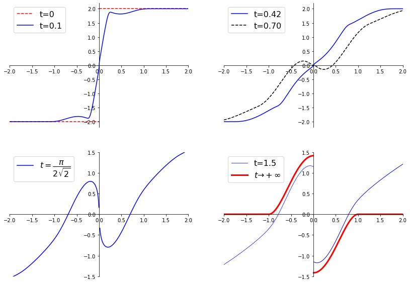
Refer to caption
Figure 2: Numerically computed solution to (CL) with HH as in (10) and initial datum (11), as described in Theorem 2.2. The Riemann initial datum (11) first evolves similarly to a rarefaction (top left); then gets non monotone (top right); at time t=π/(2​2)t=\pi/(2\sqrt{2}) a shock is formed (bottom left) and in subsequent times the size of the shock grows (bottom right). The latter graph also portrays the asymptotic profile (12).

Therefore, there exist an xx-dependent Hamiltonian HH, a profile ww and a time T>0T>0 such that ITC​L​(w)≠∅I^{CL}_{T}(w)\neq\emptyset but in any solution evolving from an initial datum in ITC​L​(w)I^{CL}_{T}(w), shocks arise before time TT, so that no reversible solution is possible, see Figure 4. In other words, the profile ww can be reached exclusively producing a sufficient amount of entropy and no isentropic solution evolves into ww. Each of these facts requires HH to depend on xx and is false in an xx-independent setting. As a consequence, no direct definition of uo∗u_{o}^{*} is available, as it was in the xx-independent case, explaining why in CPS2023 the authors had to resort to (HJ) for its construction.

A further difference between the homogeneous and the non homogeneous cases is in the long time behavior.

Theorem 2.3

Let HH be as in (10), choose

uo​(x)≔{−2if ​x<02if ​x>0,u_{o}(x)\coloneqq\left\{\begin{array}[]{cl}-2&\text{if }x<0\\ 2&\text{if }x>0\,,\end{array}\right. (11)

and consider the corresponding entropy solution uu to (CL). Then, for all x∈ℝ\{0}x\in{\mathbb{R}}\backslash\{0\},

limt→+∞u(t,x)=−sgnx2​(1−g​(x))={−2sgnx(1−x2)2|x|≤1,0|x|>1.\lim_{t\to+\infty}u(t,x)=-{\mathop{\rm sgn}}\,x\;\sqrt{2(1-g(x))}=\left\{\begin{array}[]{l@{\qquad}r@{\,}c@{\,}l}-\sqrt{2}\,{\mathop{\rm sgn}}\,x\;(1-x^{2})^{2}&|x|&\leq&1\,,\\ 0&|x|&>&1\,.\end{array}\right. (12)

The proof is sketched in Section 4, refer to Figure 2, bottom right, for the graph of (12).

In particular, note that a stationary shock is present at x=0x=0 in the time asymptotic limit. Outside this shock, the solution is classical.

3 Theorem 2.2 – Sketch of the Proof

Note first that HH, as defined in (10), satisfies (C3), (1) with X=1X=1 and (1).

Here follows a sequence of lemmas describing the behaviors of the solutions to (HS)– (10). The proofs, relying on standard ODE arguments, can be found in CPS2023. We refer to Figure 3 for an illustration of these behaviors.

Lemma 1

(CPS2023, Lemma 5.11) Let HH be as in (10) and uou_{o} be as in (11). Fix qo≥0q_{o}\geq 0. Denote by (q,p)(q,p) the solution to (HS)–(10) with initial datum (qo,uo​(qo+))=(qo,2)\left(q_{o},u_{o}(q_{o}+)\right)=(q_{o},2). Then, qq is increasing on [0,+∞[[0,+\infty\mathclose{[} and q⁡(t)​⟶t→+∞+∞q(t){\ \underset{t\to+\infty}{\longrightarrow}\ }+\infty.

Lemma 2

(CPS2023, Lemma 5.12) Let HH be as in (10) and uou_{o} be as in (11). Fix 0≤qo<qo~0\leq q_{o}<\widetilde{q_{o}} and denote by (q,p)(q,p), respectively (q~,p~)(\widetilde{q},\widetilde{p}), the global solution to (HS)–(10) with initial datum (qo,uo​(qo+))=(qo,2)\left(q_{o},u_{o}(q_{o}+)\right)=(q_{o},2), respectively (qo~,uo​(qo~+))=(qo~,2)\left(\widetilde{q_{o}},u_{o}(\widetilde{q_{o}}+)\right)=(\widetilde{q_{o}},2). Then, q​(t)<q~​(t)q(t)<\widetilde{q}(t), for all t≥0t\geq 0.

Lemma 3

(CPS2023, Lemmas 5.13 – 5.15) Let HH be as in (10) and uou_{o} be as in (11). Fix po∈]0,2[p_{o}\in\mathopen{]}0,2\mathclose{[}. Denote by (q,p)(q,p) the global solution to (HS)–(10) with initial datum (0,po)(0,p_{o}).
(i) If po∈]2,2[p_{o}\in\mathopen{]}\sqrt{2},2\mathclose{[}, then qq is increasing on [0,+∞[[0,+\infty\mathclose{[} and q⁡(t)​⟶t→+∞+∞q(t){\ \underset{t\to+\infty}{\longrightarrow}\ }+\infty.
(ii) If po=2p_{o}=\sqrt{2}, then qq is increasing on [0,+∞[[0,+\infty\mathclose{[} and q⁡(t)​⟶t→+∞​ 1q(t){\ \underset{t\to+\infty}{\longrightarrow}\ }1.
(iii) If po∈]0,2[p_{o}\in\mathopen{]}0,\sqrt{2}\mathclose{[}, then qq is periodic and the map

𝒯:]0,2[⟶]0,+∞[po⟼the smallest period of q\begin{array}[]{l@{\,}ccc}\mathcal{T}\colon&\mathopen{]}0,\sqrt{2}\mathclose{[}&\longrightarrow&\mathclose{]}0,+\infty\mathclose{[}\\ &\displaystyle{p_{o}}&\longmapsto&\displaystyle{\text{the smallest period of $q$}}\end{array} (13)

is increasing, continuous and limpo→2𝒯⁡(po)=+∞\lim_{p_{o}\to\sqrt{2}}\mathcal{T}(p_{o})=+\infty. Moreover, q⁡(t)>0q(t)>0 for t∈]0,𝒯(po)/2[t\in\mathopen{]}0,\mathcal{T}(p_{o})/2\mathclose{[} and q⁡(t)<0q(t)<0 for t∈]𝒯(po)/2,𝒯(po)[t\in\mathopen{]}\mathcal{T}(p_{o})/2,\mathcal{T}(p_{o})\mathclose{[}.

Lemma 4

(CPS2023, Lemma 5.16) Let HH be as in (10) and uou_{o} be as in (11). Fix 0<po<po~<20<p_{o}<\widetilde{p_{o}}<2 and denote by (q,p)(q,p), respectively (q~,p~)(\widetilde{q},\widetilde{p}), the global solution to (HS)–(10) with initial datum (0,po)(0,p_{o}), respectively (0,po~)(0,\widetilde{p_{o}}). Then,

(i)\displaystyle(i) po∈]0,2[⟹∀t∈]0,𝒯(po)/2],q(t)<q~(t)\displaystyle p_{o}\in]0,\sqrt{2}[\implies\forall t\in\mathopen{]}0,\mathcal{T}(p_{o})/2],\;q(t)<\widetilde{q}(t)
(i​i)\displaystyle(ii) po∈[2,2[⟹∀t∈]0,+∞[,q(t)<q~(t).\displaystyle p_{o}\in[\sqrt{2},2[\implies\forall t\in]0,+\infty[,\;q(t)<\widetilde{q}(t).
Refer to caption
Figure 3: On the horizontal axis, the qq component of solutions to (HS)–(10), while time tt is on the vertical axis. Dotted curves are those considered in Lemma 1 and in Lemma 2; dashed-dotted curves are those considered in (i) of Lemma 3; solid curves refer to (iii) of Lemma 3. The two thicker curves depict solutions corresponding to the initial data (0,2)(0,\sqrt{2}) and (0,2)(0,2).

Recall that (C3)-(1)-(1) ensure that for all (qo,po)∈ℝ2(q_{o},p_{o})\in{\mathbb{R}}^{2}, calling (q,p)(q,p) the solution to (HS)–(10) with datum (qo,po)(q_{o},p_{o}) at time 00, the map

ℱ:ℝ3⟶ℝ2(t,qo,po)⟼(q⁡(t),p⁡(t))\begin{array}[]{l@{\,}ccc}\mathcal{F}\colon&{\mathbb{R}}^{3}&\longrightarrow&{\mathbb{R}}^{2}\\ &\displaystyle{(t,q_{o},p_{o})}&\longmapsto&\displaystyle{\left(q(t),p(t)\right)}\end{array} (14)

and its two projections ℱq,ℱp\mathcal{F}_{q},\mathcal{F}_{p} are of class 𝐂2\mathbf{C}^{2}, see (CPS2023, Lemma 5.2).

Lemma 5

(CPS2023, Lemma 5.17) Let HH be as in (10) and uou_{o} be as in (11). Then, there exists a unique map

Δ:]0,+∞[2⟶([0,+∞[×{2})∪({0}×]0,2])(t,x)⟼(qo,po)\begin{array}[]{l@{\,}ccc}\Delta\colon&\mathopen{]}0,+\infty\mathclose{[}^{2}&\longrightarrow&\left([0,+\infty\mathclose{[}\times\{2\}\right)\cup\left(\{0\}\times\mathopen{]}0,2]\right)\\ &\displaystyle{(t,x)}&\longmapsto&\displaystyle{(q_{o},p_{o})}\end{array} (15)

such that

ℱq(t,qo,po)=xand∀s∈]0,t[,ℱq(s,qo,po)>0.\mathcal{F}_{q}(t,q_{o},p_{o})=x\quad\text{and}\quad\forall\,s\in\mathopen{]}0,t\mathclose{[},\;\mathcal{F}_{q}(s,q_{o},p_{o})>0\,. (16)

Moreover,
(i) Δ\Delta is continuous.
(ii) Δ\Delta is monotone, in the sense that setting Δ⁡(to,xo)=(0,po)\Delta(t_{o},x_{o})=(0,p_{o}) and Δ⁡(to,xo′)=(0,po′)\Delta(t_{o},x_{o}^{\prime})=(0,p_{o}^{\prime}), if 0<xo<xo′0<x_{o}<x_{o}^{\prime}, then po<po′p_{o}<p_{o}^{\prime}.
(iii) For all x∈]0,+∞[x\in\mathopen{]}0,+\infty\mathclose{[}, limt→0+Δ⁡(t,x)=(x,2)\lim_{t\to 0+}\Delta(t,x)=(x,2).

The construction of the solution to (CL)–(11) now follows from the next proposition.

Proposition 1

(CPS2023, Proposition 5.18) Let HH be as in (10) and uou_{o} as in (11). Then,

u:]0,+∞[×(ℝ∖{0})⟶ℝ(t,x)⟼{ℱp​(t,Δ​(t,x))ifx>0−ℱp​(t,Δ⁡(t,−x))ifx<0.\begin{array}[]{l@{\,}ccc}u\colon&\mathopen{]}0,+\infty\mathclose{[}\times({\mathbb{R}}\setminus\{0\})&\longrightarrow&{\mathbb{R}}\\ &\displaystyle{(t,x)}&\longmapsto&\displaystyle{\left\{\begin{array}[]{ccl}\mathcal{F}_{p}\left(t,\Delta(t,x)\right)&\text{if}&x>0\\[5.0pt] -\mathcal{F}_{p}\left(t,\Delta(t,-x)\right)&\text{if}&x<0.\end{array}\right.}\end{array} (17)

is the solution to (CL) in the sense of Definition 1 and it is a classical solution outside x=0x=0.

We refer to (CPS2023, § 5.4) for the concluding remarks proving the properties of uu.

Refer to caption
Figure 4: Illustration of Proposition 1: evolution in time of the solution to (CL) in connection with the orbits of (HS)–(10).

4 Proof of Theorem 2.3

Since uu is odd in the space variable, we consider only the case x>0x>0. Using the notation (14), introduce the maps

q♭​(t)=ℱq​(t,0,2) and q♯​(t)=ℱq​(t,0,2)q^{\flat}(t)=\mathcal{F}_{q}(t,0,\sqrt{2})\quad\mbox{ and }\quad q^{\sharp}(t)=\mathcal{F}_{q}(t,0,2) (18)

whose graphs are thicker in Figure 3. By Lemma 1 and Lemma 3, limt→+∞q♭​(t)=1\lim_{t\to+\infty}q^{\flat}(t)=1 and limt→+∞q♯​(t)=+∞\lim_{t\to+\infty}q^{\sharp}(t)=+\infty.

Assume first x∈]0,1[x\in\mathopen{]}0,1\mathclose{[}. Then, if t>(q♭)−1​(x)t>(q^{\flat})^{-1}(x), by (ii) in Lemma 3 and (ii) in Lemma 5, Δ⁡(t,x)=(0,po​(t,x))\Delta(t,x)=(0,p_{o}(t,x)) for a suitable po(t,x)∈]0,2[p_{o}(t,x)\in\mathopen{]}0,\sqrt{2}\mathclose{[}. Moreover, by (16) in Lemma 5 and (iii) in Lemma 3, t<𝒯⁡(po​(t,x))/2t<\mathcal{T}(p_{o}(t,x))/2. Hence, as t→+∞t\to+\infty, also 𝒯⁡(po​(t,x))→+∞\mathcal{T}(p_{o}(t,x))\to+\infty. By (iii) in Lemma 3, limt→+∞po​(t,x)=2\lim_{t\to+\infty}p_{o}(t,x)=\sqrt{2}.

Assume now that x≥1x\geq 1. If t>(q♯)−1​(x)t>(q^{\sharp})^{-1}(x), by Lemma 1, Δ⁡(t,x)=(0,po​(t,x))\Delta(t,x)=(0,p_{o}(t,x)) with po(t,x)∈[2,2[p_{o}(t,x)\in[\sqrt{2},2\mathclose{[}. By (ii) in Lemma 4 and (i) in Lemma 3, we have limt→+∞po​(t,x)=2\lim_{t\to+\infty}p_{o}(t,x)=\sqrt{2}.

Recall that along solutions to (HS)–(10), HH is conserved, that is

u​(t,x)22+g⁡(x)=po​(t,x)22+g⁡(0),\frac{u(t,x)^{2}}{2}+g(x)=\frac{p_{o}(t,x)^{2}}{2}+g(0)\,, (19)

so that

limt→+∞u​(t,x)2=2​(1−g⁡(x))≥0,\lim_{t\to+\infty}u(t,x)^{2}=2(1-g(x))\geq 0\,, (20)

proving (12) for x≥1x\geq 1.

For x∈[0,1[x\in[0,1\mathclose{[}, we proved above that, for tt large, po(t,x)∈]0,2[p_{o}(t,x)\in\mathopen{]}0,\sqrt{2}\mathclose{[}. This, together with (19) ensures that

u⁡(t,x)<2​(1−g​(x)).u(t,x)<\sqrt{2(1-g(x))}\,. (21)

By (CL), understood in its classical sense thanks to Proposition 1, and by (19)

∂tu(t,x)=−∂x(H(x,u(t,x)))=−∂x(po​(t,x)22)=−po(t,x)∂xpo(t,x).\partial_{t}u(t,x)=-\partial_{x}\left(H\left(x,u(t,x)\right)\right)=-\partial_{x}\left(\frac{p_{o}(t,x)^{2}}{2}\right)=-p_{o}(t,x)\;\partial_{x}p_{o}(t,x)\,.

Indeed, note first that by (19), po​(t,x)>0p_{o}(t,x)>0 and the Implicit Function Theorem, pop_{o} is sufficiently regular. Item (ii) in Lemma 5 implies that ∂xpo​(t,x)≥0\partial_{x}p_{o}(t,x)\geq 0, so that ∂tu⁡(t,x)≤0\partial_{t}u(t,x)\leq 0. Hence, (20) and (21) allow to complete the proof of (12).

As a final remark, we note that as t→+∞t\to+\infty, u⁡(t)u(t) converges uniformly on compact subsets of ℝ∖{0}{\mathbb{R}}\setminus\{0\}, thanks to pointwise convergence and monotonicity, by Dini’s Theorem (zbMATH03539473, Theorem 7.13). A further technical argument, based on (ii) of Theorem 2.2, allows to extend the local uniform convergence on all of ℝ{\mathbb{R}}.

Acknowledgements.
The first author was partly supported by the GNAMPA 2022 project Evolution Equations, Well Posedness, Control and Applications. This research was funded, in whole or in part, by l’Agence Nationale de la Recherche (ANR), project ANR-22-CE40-0010. For the purpose of open access, the second author has applied a CC-BY public copyright license to any Author Accepted Manuscript (AAM) version arising from this submission.

References

  • [1] Adimurthi and S. S. Ghoshal. Exact and optimal controllability for scalar conservation laws with discontinuous flux, 2020.
  • [2] F. Ancona and M. T. Chiri. Attainable profiles for conservation laws with flux function spatially discontinuous at a single point. ESAIM Control Optim. Calc. Var., 26:Paper No. 124, 33, 2020.
  • [3] F. Ancona and A. Marson. On the attainable set for scalar nonlinear conservation laws with boundary control. SIAM J. Control Optim., 36(1):290–312, 1998.
  • [4] E. N. Barron, P. Cannarsa, R. Jensen, and C. Sinestrari. Regularity of Hamilton-Jacobi equations when forward is backward. Indiana Univ. Math. J., 48(2):385–409, 1999.
  • [5] R. M. Colombo and V. Perrollaz. Initial data identification in conservation laws and Hamilton–Jacobi equations. J. Math. Pures et Appl., 138:1–27, 2020.
  • [6] R. M. Colombo, V. Perrollaz, and A. Sylla. Conservation laws and Hamilton–Jacobi equations with space inhomogeneity. Preprint, 2022. https://hal.archives-ouvertes.fr/hal-03873174.
  • [7] R. M. Colombo, V. Perrollaz, and A. Sylla. Initial Data Identification in Space Dependent Conservation Laws and Hamilton-Jacobi Equations. Preprint, 2023. https://hal.science/hal-04062783.
  • [8] C. M. Dafermos. Generalized characteristics and the structure of solutions of hyperbolic conservation laws. Indiana University Mathematics Journal, 26(6):1097–1119, 1977.
  • [9] C. Esteve-Yagüe and E. Zuazua. Reachable set for Hamilton-Jacobi equations with non-smooth Hamiltonian and scalar conservation laws. Nonlinear Anal., 227:Paper No. 113167, 2023.
  • [10] L. Gosse and E. Zuazua. Filtered gradient algorithms for inverse design problems of one-dimensional Burgers equation. In Innovative algorithms and analysis, volume 16 of Springer INdAM Ser., pages 197–227. Springer, Cham, 2017.
  • [11] S. N. Kruzhkov. First order quasilinear equations with several independent variables. Mathematics of the USSR-Sbornik, 81(123):228–255, 1970.
  • [12] T. Liard and E. Zuazua. Initial data identification for the one-dimensional Burgers equation. IEEE Transactions on Automatic Control, 2021.
  • [13] W. Rudin. Principles of mathematical analysis. 3rd ed. International Series in Pure and Applied Mathematics. Düsseldorf etc.: McGraw-Hill Book Company. X, p.342, 1976.