ReSDF: Redistancing Implicit Surfaces using Neural Networks
Abstract
This paper proposes a deep-learning-based method for recovering a signed distance function (SDF) of a given hypersurface represented by an implicit level set function. Using the flexibility of constructing a neural network, we use an augmented network by defining an auxiliary output to represent the gradient of the SDF. There are three advantages of the augmented network; (i) the target interface is accurately captured, (ii) the gradient has a unit norm, and (iii) two outputs are approximated by a single network. Moreover, unlike a conventional loss term which uses a residual of the eikonal equation, a novel training objective consisting of three loss terms is designed. The first loss function enforces a pointwise matching between two outputs of the augmented network. The second loss function leveraged by a geometric characteristic of the SDF imposes the shortest path obtained by the gradient. The third loss function regularizes a singularity of the SDF caused by discontinuities of the gradient. Numerical results across a wide range of complex and irregular interfaces in two and three-dimensional domains confirm the effectiveness and accuracy of the proposed method. We also compare the results of the proposed method with physics-informed neural networks approaches and the fast marching method.
Keywords:
Signed distance function; Level set function; Reinitialization; Deep learning; Eikonal equation1 Introduction
The signed distance function (SDF) to a hypersurface , which is the distance to in the outer region and the negative of the distance to in the inner region, has been crucial in various fields, ranging from computational fluid dynamics [1, 2, 3] to image segmentation [4, 5, 6], 3D shape reconstruction from scattered point data [7, 8, 9], architectural geometry [10, 11], and robotic navigation [12, 13]. After being devised by Osher and Sethian [14], the level set method, which represents as the zero level set of a continuous function , provides a numerical and theoretical paradigm of evolving hypersurfaces. To facilitate geometric features such as the normal vector and mean curvature of the interface and to reduce numerical instability, the level set function is preferable to be neither too flat nor steep near its zero contours. Reinitializing it as the SDF has been a common numerical treatment in modelling the motion of dynamic interfaces [15, 16, 17, 18] and shape optimization [19, 20, 21, 22].
There have been several numerical methods to re-distance the given level set function . One of the most prominent efforts is built on the fact that the SDF is a solution of partial differential equations (PDEs) [23, 24]. Fast marching methods (FMMs) [25, 26, 27, 28, 29] and fast sweeping methods [30, 31, 32] recover the SDF as a viscosity solution to the eikonal equation. Sussman et al. [33] reformulated the eikonal equation by a pseudo-time-dependent nonlinear hyperbolic PDE. This approach is known to be more suitable than solving directly the eikonal equation in the case of evolving interfaces. Since the SDF [33] is obtained by the stationary solution, it is time-consuming and requires a large number of iterations depending on the CFL restriction. A more serious issue is that the zero level set fails to be maintained. Lee et al. [34] propose a fast method by using the Hopf-Lax formula of the Hamilton-Jacobi equation. In [35], it is known that the solution of the Hamilton-Jacobi equation in [34] is not exactly the SDF. Another approach [36] employs Varadhan’s distance function [37]. By the Hopf-Cole formula, it can be transformed into a regularized eikonal equation with an artificial viscosity term.
Inspired by the tremendous success of deep learning in diverse machine learning tasks, such as image classification [38, 39, 40, 41, 42] and density estimation [43, 44, 45, 46], the use of neural networks for solving PDEs has begun to attract significant attention in recent years. Pioneering studies [47, 48] incorporate physical principles into neural networks by directly constructing a loss function as a residual of PDEs and errors of boundary or initial conditions. Building upon these earlier works, Raissi et al. [49] have revisited them by using modern computational tools and provided a framework named physics-informed neural networks (PINNs). The advantage of PINNs is that they can be readily transformed into various problems [50, 51, 52] and can treat the PDE in a fully mesh-free and time-continuous manner. However, they suffer from a challenging optimization landscape [53, 54], as it is difficult for them to learn many multi-scale or complex PDE systems [55, 56]. Another line of work involves neural operators [57, 58, 59], which unveil physical systems from data by learning implicit solution operator that maps boundary or initial conditions to solutions. They have shown promise in learning complex PDEs [60, 61], but the requirement for large amounts of available data limits application to various of practical problems. In addition, hybrid methods [62, 63, 64, 65] that combine deep learning with well-grounded numerical methods have been studied.

In this paper, we propose a novel method, named ReSDF, for reconstructing a SDF from a given implicit level set function whose zero level set is an interface ; see Figure 1. By exploiting flexibility of network design and optimization objectives, we compute the SDF through two major ideas. Firstly, inspired by the variable-splitting scheme [66, 67], we introduce an augmented neural network that parametrizes the gradient of the SDF as an auxiliary variable while keeping the number of network parameters. The network is designed so that the approximating SDF accurately distinguishes the interface from the interior and the outer regions and the gradient has a unit norm. Secondly, we propose a training objective consisting of three loss terms. The first loss function comes from the splitting method and it enforces matching vectors between the gradient of the estimated SDF and the auxiliary gradient. The second loss function imposes a geometric fact that the gradient of the SDF defines the shortest path to the interface. The third loss function is devised to alleviate the nonuniqueness of the gradient caused by multiple shortest paths at a singular point of the SDF. We also provide a theoretical validation of the proposed objectives for reinitializing a level set function. Numerical results confirm that proposed loss functions in conjunction with the designed neural network significantly improve the accuracy compared to the existing PINN approach. The ReSDF also accurately approximates the SDF for the cases of complex and irregular interfaces without tuning sensitive hyper-parameters. The capability of the model is also tested to estimate the distance function on three-dimensional space without increment in the number of parameters of the network.
The rest of the paper is organized as follows. In Section 2, we present the formulation of the problem and a brief discussion about prior works. In Section 3, we introduce the proposed ReSDF by describing the augmented network and the objective function in detail. Numerical experiments are presented in Section 4 to demonstrate the effectiveness and accuracy of ReSDF, followed by some concluding remarks given in Section 5.
2 Previous Works
Let be a domain and be a compact hypersurface implicitly represented by a zero level set of a continuous level set function . The hypersurface divides into two disjoint open subsets: the outer region and the inner region satisfying . From the given function , the goal is to find the signed distance function (SDF) that satisfies
| (1) |
where denotes the standard Euclidean distance function to . It is a unique viscosity solution to the eikonal equation [68]
| (2) | ||||
| (3) |
where is the given level set function and sgn is the signum function, which takes either , , or for points in , , or , respectively.
The variational approaches to approximate the distance function (2) in [69, 70, 71] are to minimize the energy functional related to the eikonal equation:
| (4) |
in conjunction with the Dirichlet boundary condition as a constraint relaxed by a penalty term:
| (5) |
Several efforts have also been made to improve the ill-posedness or convergence of the variational problem (4), including penality methods introducing external energy functionals for shifting the zero level set toward the target interface [6] and for preserving the shape of the free interface [72], and effective splitting schemes [36, 73] using alternating direction method of multipliers [74].
As neural PDE surrogates have proliferated as an impactful area of research, several efforts have been made to reconstruct the SDF using neural networks. Prior studies mostly resort to the steady eikonal equation to find the SDF. Lichtenstein et al. [75] propose a hybrid method that integrates neural networks into the FMM [25]. They replace the local numerical solver in the FMM with a neural network trained from data. The accuracy of the numerical solution is improved by leveraging the expressive power of neural networks. Since the approach requires a wealth of training data with true distance values, it might be difficult to be used in application where lots of true distances are hard to obtain. The performance relies on the amount of available data and would be unfavourable outside of the data on which the network is trained. Another approach directly uses a neural network to parametrize the SDF. Gropp et al. [8] adopt the PINN approach to learn the SDF from an unorganized cloud of points. They directly use a neural network to parametrize the SDF of the given point cloud by minimizing the eikonal-embedded loss function.
Recent works [76, 77] leverage a framework of PINN [49]. Similar to the variational approaches (4), they convert the problem of solving the eikonal equation (2) into an optimization problem in which the loss function embeds the knowledge of (2):
| (6) |
where is a neural network parametrized by , which is an approximator of the solution to (2). The soft penalty term enforces an additional constraint on the solution such as weight normalization or boundary conditions. The expectation is taken with respect to a collection of scattered collocation points usually chosen by uniform random sampling. The objective of the residual of the eikonal equation characterizes the deviation of from the SDF. The trained network serves as a suitable approximation of the solution. Fayolle [76] also suggests an alternative PINN-based approach that relies on -Poisson distances [78]. As discussed in the numerical section, we compare the proposed method with the results of the PINN-based approach for irregular and complex interfaces and check the robustness of using various initial level set functions .
3 Proposed Method
In this section, we propose a learning-based approach to recover the SDF (ReSDF) of a given hypersurface implicitly represented by a level set function. In order to increase the expressiveness of the network we use an augmented network that parameterizes the gradient of SDF as an auxiliary output while keeping the number of parameters. Moreoever, novel objectives are designed to exploit a global property and alleviate a singularity of the SDF by harnessing the geometric properties of the SDF.
3.1 Augmented Network Representation
In this section, inspired by variable-splitting methods [66, 67] in optimization, an augmented network structure is considered to separately parametrize the gradient of the SDF as an auxiliary variable. The augmented network has two outputs that satisfy the following characteristics: (i) the primary output approximates the SDF and it automatically vanishes on the interface as well as satisfies the sign condition (3) and (ii) the gradient field represented by the auxiliary output has a unit norm; see Figure 2.
We parameterize a single network to output together with an auxiliary value
| (7) |
because it is more efficient to approximate the SDF and its gradient using a single common network rather than learning with two individual networks. The first scalar function and the other vector-valued component are employed to parametrize and , respectively, through a designed architecture in Figure 2. The neural perceptron is defined using a multi-layer fully-connected neural network:
where is a given depth, is a weight of the output layer, is a final bias vector and the perceptron (also known as the hidden layer) is defined by
for , , and a non-linear activation function . The dimensions of the hidden layers are also called by the width of the network. As the input to the network is a point in , the input dimension of the input layer is . The output layer recovers the -dimensional output values using the matrix product between the output of the final hidden layer and in addition to a bias vector . A shorthand notation is used for all parameters in the weights and biases . Given the current parameter configuration, the parameters are successively adapted by minimizing an assigned loss function explained in Section 3.2.
Representation of SDF
We aim to adjust the network output so that the approximated SDF satisfies the sign condition (3). Thanks to the level set representation, the sign of the SDF is easily obtained. Similar to [76], we treat the condition on the sign of the SDF as a hard constraint by parameterizing the primary output as
| (8) |
where the quantity is a smoothed sign function of :
with a scaling factor and a smoothing parameter are fixed in all examples. Clearly, the designed artificial neural network as an ansatz of the SDF automatically brings the sign condition, . In particular, vanishes on the target interface . Therefore, the zero-level set of the approximated SDF can accurately preserve the interface without smearing out.
Approximation of the gradient field
In contrast to the existing approaches, which treat the unit norm property of the gradient as a soft constraint, we design the augmented output
to automatically satisfy the unit norm constraint. To this end, we define a neural network that lies in the unit sphere by normalizing the auxiliary output :
| (9) |
In other words, learns only the direction of the gradient of SDF and it is automatically adjusted to the unit length by normalization.
To sum up, the SDF and its gradient are estimated from the output of the augmented network (7) as
| (10) | ||||
| (11) |
The resultant vanishes on and has unit length. Moreover, it is worth emphasizing that and share the same weights and biases from the input layer till the last hidden layer. This enables a reduction in the number of parameters and faster training than using two separate networks.
3.2 Design of loss functions
A formulation of the loss function is another key ingredient to achieve effective learning using two outputs of the augmented networks (7). In this section, we explain the following objective function consisting of three loss terms:
| (12) |
where is a fixed constant. The main characteristics are summarized:
- •
The first term enforces the vector matching between the gradient of the primary output and the auxiliary output.
- •
The second term imposes a global property using the fact that the SDF and its gradient determine the shortest path to the interface.
- •
The third term alleviates a singularity where the SDF is not differentiable.
In A, it is proved that the SDF is a minimizer of the functional . The Euler-Lagrange equation for the functional is nonlinear and it is not straightforward to find a minimizer by conventional methods. It highlights one of the main advantages of the deep learning approach to minimize such a complex loss function.
Gradient matching objective
The gradient matching (GM) objective directly enforces to reduce a gap between the gradient of the primary output and the unit-norm auxiliary output in (7):
| (13) |
The gradient of in (13) by auto-differentiation library (autograd) [79] calculates the exact derivatives of the networks. In the view of the variable-splitting method, the variational problem (5) is reformulated by
By regularizing the constraint as a penalty term, an unconstrained problem is presented:
| (14) |
where is a regularization parameter. Since automatically vanishes on in the proposed network structure in Section 3.1, the first loss term in (14) is no longer needed. The network structure in which the is designed to have a unit norm allows us to exclude the second term in (14). This leads us to consider (13). Since the existing PINN methods are used to learn the eikonal equation with a single network output, the network must learn the direction of the gradient while matching its norm to be one. In the matching loss function (13), learns the direction of the gradient of the SDF and is matched pointwise to the normalized vector of .
Shortest path objective
The shortest path (SP) objective explains how the gradient of SDF makes the shortest path to the interface :
| (15) |
The loss function specifies a relations between the interface and the points away from by using the gradient of the SDF. The following proposition delivers a justification of using (15) in the view of geometric property of the SDF.
Proposition 1.
The property (16) describes the shortest path of a point to the target interface. The shortest path explains that a point came from a point on the interface , that is, the closest point to on . Note that (13) matches a local relation between the gradient of and pointwisely. On the other hand, the shortest path loss function dictates non-local relation between points and directly enforces to satisfy the geometric property along with . With a help of a given function whose zero level set represents , we have
| (17) |
then in the loss function (15) is a reasonable choice and train it to approach zero. Note that this loss function requires the derivative of with respect to the spatial variable and the computed gradient is multiplied by again. It is a challenging optimization because the gradient calculation is deep and the loss landscape is complex. However, as we have as an approximation of the gradient of the SDF, we replace with in (17). By replacing with , the chain rule for computing the gradients of the objective (15) is simpler than using .
Regularizing singularity objective
The regularizing singularity (RS) objective resolves a singularity of the SDF:
| (18) |
where . At a singular point , since there are multiple closest points (16) on the interface, the gradient of the SDF at is not unique. In (18), we detour the singularity of the SDF by defining at a singular point as a reliable gradient value near the interface for some . The idea is supported by the following proposition.
Proposition 2.
Let be a compact hypersurface of a domain and the signed distance function to . For any point where is differentiable, the gradient of is constant along the ray emanating from in direction :
The proof is provided in B. In practice, as in , we replace with and we set so that the point gets close to the target interface having reliable gradient value. The loss function enables accurate and stable training of and provides an appropriate approximation of SDF for various irregular interfaces.
To sum up, the proposed ReSDF optimizes the augmented network through the objective
| (19) |
It can be extended to the weighted sum of each loss term where the positive regularization parameters balance the role of each. We may impose a larger weight on the larger component to accelerate its convergence. A more provable alternative to hand-tuned weights is the use of adaptive regularization parameter methods [82, 53, 83]. However, in contrast to most PINN methods, which are sensitive to the regularization parameter, we experimentally confirm that the objective (19) is transferable across a wide variety of interfaces and level set functions .
3.3 Numerical Considerations
There are a few numerical considerations to clarify the implementation of the proposed method. In order to minimize biased training of the neural network proportional to the values of , we consider the following normalization of
where the maximum is computed over points in . The values of over the entire computational domain are balanced in the objective and the normalization alleviates the imbalance of and enables the model to recover the SDF well from the strongly distorted level set function . To remove a singularity caused by the absolute value function in (8), we use a smooth approximation. For a point at which , we define a quadratic approximation
where is chosen such that , and is taken so that is continuous at . Moreover, we adopt the leaky rectified linear unit (LeakyReLU) activation function:
which is possibly a good representation for a non-smooth function.
The second term of the loss functions has a complex form in which the network is composited within the network. It causes practical difficulties in optimization when the loss function has a stacked network. In the implementation, we optimize as follows:
where we do not update the network by disabling the gradient calculation of . Then, the computational graph is no longer associated with the parameters of and it is regarded as a fixed function in the loss function.
The SDF is Lipschitz continuous with the Lipschitz constant . In the multilayer perceptron structure approximating , the activation function and weights determine the Lipschitz condition of the approximated SDF. Since we are using LeakyReLU whose Lipschitz conatant is 1 as an activation function, we can obtain the desired condition by adjusting the weights. The commonly used method to enforce the Lipschitz condition is weight clipping [84]. It clamps the weights to a bounded box after each gradient update. In the implementation, the clipping parameter is used.
4 Numerical Results
In this section, we present numerical results of ReSDF on several problems to validate the effectiveness and accuracy for re-distancing the given level set functions. For quantitative measurements, the accuracy of the trained model is measured by the difference with the exact solution and exact gradient using the following norms:
| (20) | ||||||||||
where is the volume of the computational domain . Since the errors on the interface are crucial for the cases of evolving the interface, we also check the errors, and , which are only measured on the interface for a few examples. For qualitative comparison, the results of ReSDF are compared with the existing PINN approach and the first [25] and second-order [85] fast marching method (FMM), where implementation builds on an open-source code 11 1 https://github.com/scikit-fmm/scikit-fmm. The PINN method based on [76] uses the residual of the eikonal equation (6) as the loss function. As suggested in [76], a fully connected network with depth and width with skip connection from the input and the fourth hidden layer are used in which all weights and biases are initialized by the geometric initialization scheme [86]. We optimize the network by Adam optimizer [87] with learning rate of . We also comply with all other experimental configurations as provided in [76]. Note that the results of the PINN approach can be improved because the performance relies on specific geometric network parameter initialization [86] and is sensitive to hyper-parameter selection.
For all examples of testing ReSDF, the Adam optimizer is applied with a learning rate of , which decayed by if the loss function does not improve after evaluations. We evaluate the models per epochs and trained them until the learning rate decayed by times. In all numerical experiments, a single NVIDIA RTX 3090 GPU is used.
 |
 |
| (a) | |
 |
 |
| (a) | |
 |
 |
| (c) | |
The computational domains of all examples are or . The collocation points evenly distributed on the domain are presented by
| (21) |
Accordingly, . All interfaces and given level set functions used in numerical examples are listed below. In case of the closed form of the exact SDF is not known for given interfaces, we approximate it by creating a finite number of points, around 7000, on the interface and finding the minimum Euclidean distance from them.
- 1.
- 2.
- 3.
- 4.
- 5.
- 6.
- 7.
A sphere centered at the origin with the radius is represented by the zero level sest of the level set function used in Example 5; see the coutours on in Figure 11-(a):
(32) Multiple ellipsoidal interfaces represented by the zero level set of minimum of the level set functions are used in Example 5; see the iso-contours on in Figure 11-(c):
(33) where and .
Example 1
| 32 | 64 | 128 | 256 | |||||
|---|---|---|---|---|---|---|---|---|
| 32 | 64 | 128 | 256 | |||||
|---|---|---|---|---|---|---|---|---|
In this example, we would like to numerically check an accuracy and robustness of the proposed model using an exact SDF (22). The accuracy of the learned solution is investigated with respect to different network sizes and batch sizes of the training data points. Numerical tests of ReSDF are performed by using the level set function defined in (23) with network widths , and collocation points with . In Table 1, the and errors (20) between the exact SDF and learned over the entire computational domain are presented. The accuracy of the obtained measured by and errors (20) on the interface between and the exact outward normal vector is summarized in Table 2. Note that only the number of collocation points and the width are changed and the other experimental settings are kept the same. The results show that the errors do not alter significantly with different batch sizes of training collocation points. Even with a coarse grid, we still obtain accurate predictions. We can also observe that the resulting errors decrease as the network width size increases. This is a general phenomenon in which the expressive power increases as the size of the network increases.
| Model | # Params | ||||||
|---|---|---|---|---|---|---|---|
| ReSDF | 17,027 | ||||||
| PINN | 1,840,641 | ||||||
 |
 |
| (a1) ReSDF with | (b1) PINN with |
 |
 |
| (a2) ReSDF with | (b2) PINN with |
 |
 |
| (a3) ReSDF with | (b3) PINN with |
The robustness of changing the level set functions is examined by using diverse initial level set functions; a stiff shape (23), an oscillatory shape (25), and a discontinuous shape (24). In this case, the model is trained with a fixed width of size on collocation points . The results are compared with that of the PINN approach. The accuracy of two models is listed in Table 3. The results of ReSDF have a smaller error than the results of the PINN approach by a factor of and in the and norms, respectively. In order to present visual differences, we compare the predictions of the trained ReSDF and PINN against the exact SDF in Figure 4. It shows a similar result with . However, the PINN approach fails to predict SDF with and .
Example 2
 |
 |
| (a) | (b) ReSDF with |
| Method | |||||
|---|---|---|---|---|---|
| ReSDF | |||||
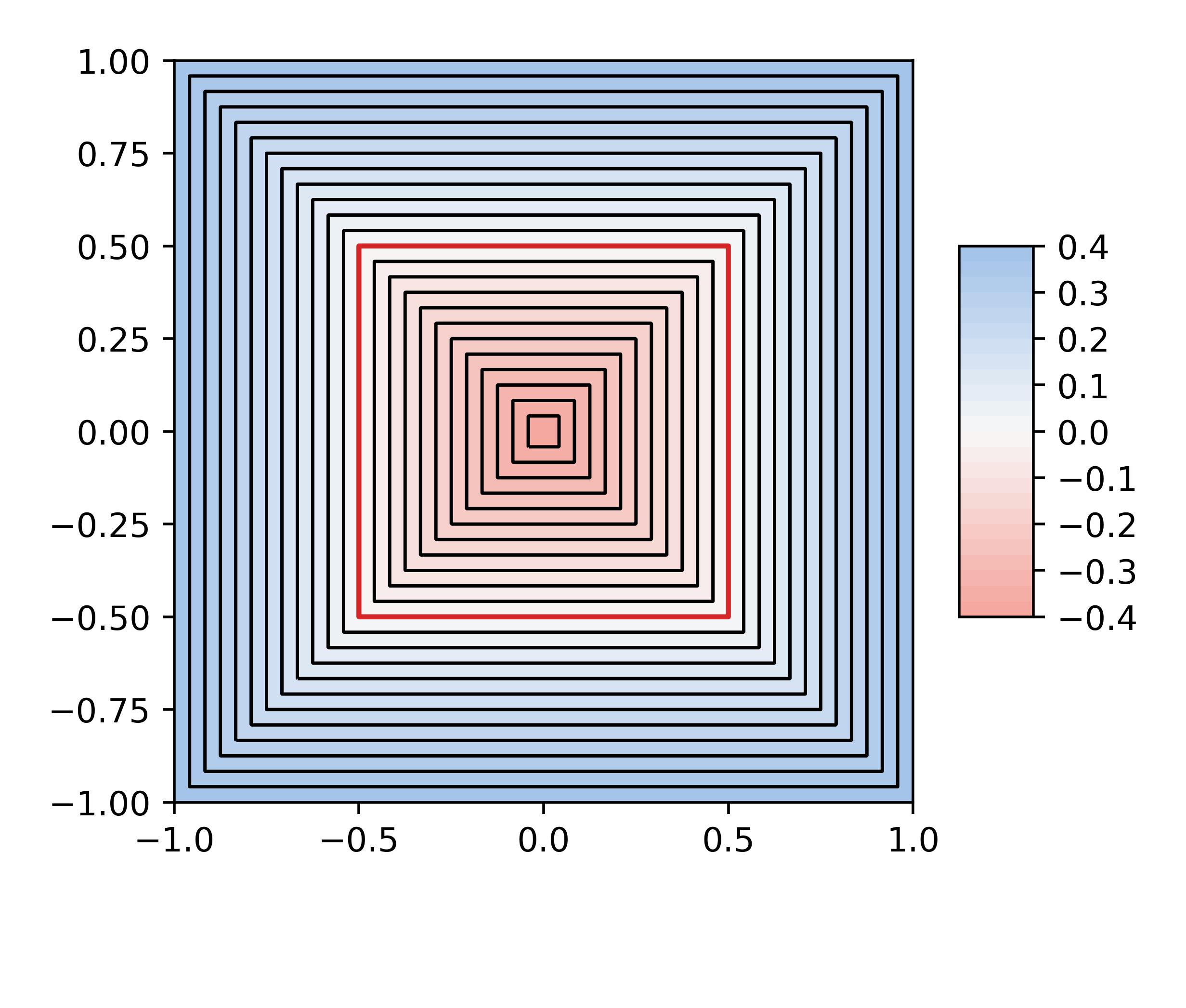
For a square-shaped interface, we would like to compare the result of ReSDF with the level set function (26) with the . The network is a -layer fully connected network with width which is trained on the collocation points . In Figure 5, the iso-contours of the level set function is presented and the exact solution and the result of ReSDF are shown. As shown in Figure 5, the exact SDF contains discontinuities of the gradient along the diagonal lines of the zero level set and the sharp corners become rounded in the outer region. The singularities arising from these sharp corners make it difficult to approximate the exact SDF. The numerical result depicted in Figure 5 confirms that the proposed model approximates both the smooth outer region and the sharp inner points. In order to see how good numerical solution it is, we compare the results with the second order FMM () in Table 4. The errors of the SDF and its gradient predicted by ReSDF on are between the errors of the result of on and . It means that the accuracy of ReSDF on a small number of collocation points is comparable to on a large number of collocation points and it is consistent with previous findings in Example 1.
Example 3
 |
 |
| (a) | (b) |
 |
 |
| (c) | (d) |
To demonstrate that the proposed model can be applied to various interfaces, the level set functions, (27) with and , (28), and (29), are used to be reinitialized; see in Figure 6. Due to the rapid change of the gradient field of the level set functions and , the clipping parameter is used to improve the representability of . Other parameters are consistent with other cases.
 |
 |
| (a1) ReSDF with | (b1) PINN with |
 |
 |
| (a2) ReSDF with | (b2) PINN with |
 |
 |
| (a3) ReSDF with | PINN with |
 |
 |
| ReSDF on | PINN on |
 |
 |
| FMM on | FMM on |
 |
 |
| FMM on | FMM on |
 |
 |
| on | on |
 |
 |
| on | on |
Throughout the examples in Figure 7, the results are compared with the existing PINN approach. The numerical results verify that the proposed method has better agreement with the exact SDF than PINN approach which is prone to returning erroneous predictions for chosen irregular interfaces. Furthermore, the result of ReSDF with the level set function 29 on is qualitatively compared with the results of FMM and on , in Figures 8 and 9, respectively. In the neural network of ReSDF, we use the width and depth . Since the batch size is small to , the learning rate is initialized by . FMM produces reliable results when the mesh is sufficiently refined. Comparing the results in Figure 8, the result of the first-order FMM on is similar to the result of ReSDF trained on the collocation points . Similarly, in Figure 9, the result of ReSDF on is a comparable to the results of the second-order FMM on between and .
Example 4
 |
 |
| (a) | (b) ReSDF with |
 |
 |
| (c) | (d) ReSDF with |
We investigate the ability of ReSDF to approximate the SDF when the interface is a union of several interfaces. Such a complex mixed interface is relevant to practical problems such as the rising of multiple bubbles in multi-phase flows. The zero level sets of the level set functions (30) or (31) could depict cases of merged bubbles or multiple bubbles in the water, respectively. In Figure 10, predicted SDFs and the exact solutions are presented. Although the SDF has singularities over the computational domain, ReSDF provides accurate interface representations for multiple nested interfaces.
| Uniform nodes | Random nodes | |||
|---|---|---|---|---|
Another strength of the deep-learning-based approach in ReSDF is that scattered collocation points can be used without any methodological modifications. We investigate the effect of the deployment of training collocation points with level set functions (30) or (31). The uniform collocation points and random points of the same number of sampled from the uniform distribution are used. Running five times with different random seeds, the average values of the and errors are reported in Table 5. The results confirm that the errors obtained by different distributions are of the same order of magnitude. In other words, it verifies that the performance of the model is not sensitively tied to the uniform distribution of the training collocation points.
Example 5
| 32 | 64 | 128 | ||||
|---|---|---|---|---|---|---|
| 32 | 64 | 128 | ||||
|---|---|---|---|---|---|---|
We demonstrate that the proposed method can be scaled into 3D. The number of training points is set as and , and the number of neurons is in each hidden layer with depth . The results of the sphere are listed in Tables 6 and 7. We can observe that ReSDF can still achieve a similar level of accuracy as before in the two-dimensional circular problem. It is important to point out that the number of parameters is similar to that of the two-dimensional case since only the input dimension of the input layer and the output dimension of the last output layer are increased by one. In contrast, the computational cost of classical numerical methods is prohibitively expensive when the dimensionality of the problem increases. Therefore, the numerical results validate the capability of the proposed method for three-dimensional problems without increasing computational complexity.
 |
 |
| (a) on | (b) ReSDF with |
 |
 |
| (c) on | (d) ReSDF with |


5 Conclusions
A novel neural approach is proposed to recover the signed distance function of a given hypersurface implicitly represented by the zero contour of a level set function. To enhance the expressive power of the neural network, an auxiliary output is employed to learn the gradient of the SDF in addition to the network output as a neural surrogate of the SDF. Two outputs of the gradient-augmented network are designed to satisfy certain properties as hard constraints. Moreover, underpinned by geometrical properties, we devise a training objective that imposes global properties between the interface and the whole computational domain and alleviates the singularity of the SDF. We confirm that the proposed method produces accurate and robust results without tunable parameter adjustments through various experimental examples ranging from highly distorted or discontinuous level set functions to complex and irregular interfaces.
6 Acknowledgements
This work was supported by the NRF grant [2021R1A2C3010887], the ICT R&D program of MSIT/IITP[1711117093, 2021-0-00077], and the European Union´s Horizon 2020 Research and Innovation Programme under the Programme SASPRO 2 COFUND Marie Sklodowska-Curie grant agreement No. 945478.
Appendix A Theoretical Justification
The following theorem proves that the SDF is the minimizer of (12) except on a set of measure zero.
Theorem 1.
Let be a hypersurface in a domain . The optimal solution to the functional (12) is the SDF to , except on a set of measure zero.
Proof.
Let be the optimal solution to the functional (12). For any point and a unit vector , define a function by
Clearly, it follows that and , because
Suppose for some and . Then, we have
which can be reformulated as
| (34) |
Recall that for the distance function , there exists a unit vector such that
which is identical to
The inequality we deduced in (34) leads to
However, because is the optimal solution, it satisfies for points at which is differentiable. Therefore, it can be written as , and hence
Combining both inequalities, we see that
concluding the proof. ∎
Appendix B Proof of Proposition 2
Proof.
For a given point , let us define a function as
It satisfies
| (35) |
where the last equation is deduced from the property (16). Also, since the signed distance function has a gradient with unit norm, we get
| (36) |
From (35) and (36), it follows that
for between to . This implies that and are parallel. This concludes
| (37) |
∎
References
- Olsson and Kreiss [2005] E. Olsson, G. Kreiss, A conservative level set method for two phase flow, Journal of computational physics 210 (2005) 225–246.
- Gibou et al. [2007] F. Gibou, L. Chen, D. Nguyen, S. Banerjee, A level set based sharp interface method for the multiphase incompressible navier–stokes equations with phase change, Journal of Computational Physics 222 (2007) 536–555.
- Roget and Sitaraman [2013] B. Roget, J. Sitaraman, Wall distance search algorithm using voxelized marching spheres, Journal of Computational Physics 241 (2013) 76–94.
- Tsai et al. [2001] A. Tsai, A. Yezzi, W. Wells, C. Tempany, D. Tucker, A. Fan, W. E. Grimson, A. Willsky, Model-based curve evolution technique for image segmentation, in: Proceedings of the 2001 IEEE Computer Society Conference on Computer Vision and Pattern Recognition. CVPR 2001, volume 1, IEEE, 2001, pp. I–I.
- Alvino et al. [2007] C. Alvino, G. Unal, G. Slabaugh, B. Peny, T. Fang, Efficient segmentation based on eikonal and diffusion equations, International Journal of Computer Mathematics 84 (2007) 1309–1324.
- Li et al. [2010] C. Li, C. Xu, C. Gui, M. D. Fox, Distance regularized level set evolution and its application to image segmentation, IEEE transactions on image processing 19 (2010) 3243–3254.
- Taubin [2012] G. Taubin, Smooth signed distance surface reconstruction and applications, in: Progress in Pattern Recognition, Image Analysis, Computer Vision, and Applications: 17th Iberoamerican Congress, CIARP 2012, Buenos Aires, Argentina, September 3-6, 2012. Proceedings 17, Springer, 2012, pp. 38–45.
- Gropp et al. [2020] A. Gropp, L. Yariv, N. Haim, M. Atzmon, Y. Lipman, Implicit geometric regularization for learning shapes, International Conference on Machine Learning (2020).
- Sitzmann et al. [2020] V. Sitzmann, E. Chan, R. Tucker, N. Snavely, G. Wetzstein, Metasdf: Meta-learning signed distance functions, Advances in Neural Information Processing Systems 33 (2020) 10136–10147.
- Pottmann et al. [2010] H. Pottmann, Q. Huang, B. Deng, A. Schiftner, M. Kilian, L. Guibas, J. Wallner, Geodesic patterns, ACM Transactions on Graphics (TOG) 29 (2010) 1–10.
- Novello et al. [2022] T. Novello, G. Schardong, L. Schirmer, V. da Silva, H. Lopes, L. Velho, Exploring differential geometry in neural implicits, Computers & Graphics 108 (2022) 49–60.
- Kimmel et al. [1998] R. Kimmel, N. Kiryati, A. M. Bruckstein, Multivalued distance maps for motion planning on surfaces with moving obstacles, IEEE Transactions on Robotics and Automation 14 (1998) 427–436.
- Lee et al. [2016] S. K. Lee, S. P. Fekete, J. McLurkin, Structured triangulation in multi-robot systems: Coverage, patrolling, voronoi partitions, and geodesic centers, The International Journal of Robotics Research 35 (2016) 1234–1260.
- Osher and Sethian [1988] S. Osher, J. A. Sethian, Fronts propagating with curvature-dependent speed: Algorithms based on hamilton-jacobi formulations, Journal of computational physics 79 (1988) 12–49.
- Sussman and Fatemi [1999] M. Sussman, E. Fatemi, An efficient, interface-preserving level set redistancing algorithm and its application to interfacial incompressible fluid flow, SIAM Journal on scientific computing 20 (1999) 1165–1191.
- Strain [1999] J. Strain, Semi-lagrangian methods for level set equations, Journal of Computational Physics 151 (1999) 498–533.
- Kang et al. [2000] M. Kang, R. P. Fedkiw, X.-D. Liu, A boundary condition capturing method for multiphase incompressible flow, Journal of Scientific Computing 15 (2000) 323–360.
- Cho et al. [2022] H. Cho, Y. Park, M. Kang, Solving incompressible navier–stokes equations on irregular domains and quadtrees by monolithic approach, Journal of Computational Physics 463 (2022) 111304.
- Osher and Santosa [2001] S. J. Osher, F. Santosa, Level set methods for optimization problems involving geometry and constraints: I. frequencies of a two-density inhomogeneous drum, Journal of Computational Physics 171 (2001) 272–288.
- Allaire et al. [2002] G. Allaire, F. Jouve, A.-M. Toader, A level-set method for shape optimization, Comptes Rendus Mathematique 334 (2002) 1125–1130.
- Wang et al. [2007] S. Wang, K. M. Lim, B. C. Khoo, M. Y. Wang, An extended level set method for shape and topology optimization, Journal of Computational Physics 221 (2007) 395–421.
- Van Dijk et al. [2013] N. P. Van Dijk, K. Maute, M. Langelaar, F. Van Keulen, Level-set methods for structural topology optimization: a review, Structural and Multidisciplinary Optimization 48 (2013) 437–472.
- Peng et al. [1999] D. Peng, B. Merriman, S. Osher, H. Zhao, M. Kang, A pde-based fast local level set method, Journal of Computational Physics 155 (1999) 410–438.
- Min [2010] C. Min, On reinitializing level set functions, Journal of computational physics 229 (2010) 2764–2772.
- Sethian [1996] J. A. Sethian, A fast marching level set method for monotonically advancing fronts., Proceedings of the National Academy of Sciences 93 (1996) 1591–1595.
- Kimmel and Sethian [1998] R. Kimmel, J. A. Sethian, Computing geodesic paths on manifolds, Proceedings of the national academy of Sciences 95 (1998) 8431–8435.
- Sethian and Vladimirsky [2000] J. A. Sethian, A. Vladimirsky, Fast methods for the eikonal and related hamilton–jacobi equations on unstructured meshes, Proceedings of the National Academy of Sciences 97 (2000) 5699–5703.
- Hassouna and Farag [2007] M. S. Hassouna, A. A. Farag, Multistencils fast marching methods: A highly accurate solution to the eikonal equation on cartesian domains, IEEE transactions on pattern analysis and machine intelligence 29 (2007) 1563–1574.
- Yang and Stern [2017] J. Yang, F. Stern, A highly scalable massively parallel fast marching method for the eikonal equation, Journal of Computational Physics 332 (2017) 333–362.
- Zhao [2005] H. Zhao, A fast sweeping method for eikonal equations, Mathematics of computation 74 (2005) 603–627.
- Qian et al. [2007] J. Qian, Y.-T. Zhang, H.-K. Zhao, Fast sweeping methods for eikonal equations on triangular meshes, SIAM Journal on Numerical Analysis 45 (2007) 83–107.
- Li et al. [2008] F. Li, C.-W. Shu, Y.-T. Zhang, H. Zhao, A second order discontinuous galerkin fast sweeping method for eikonal equations, Journal of Computational Physics 227 (2008) 8191–8208.
- Sussman et al. [1994] M. Sussman, P. Smereka, S. Osher, A level set approach for computing solutions to incompressible two-phase flow, Journal of Computational physics 114 (1994) 146–159.
- Lee et al. [2017] B. Lee, J. Darbon, S. Osher, M. Kang, Revisiting the redistancing problem using the hopf–lax formula, Journal of Computational Physics 330 (2017) 268–281.
- Barles et al. [1993] G. Barles, H. M. Soner, P. E. Souganidis, Front propagation and phase field theory, SIAM Journal on Control and Optimization 31 (1993) 439–469.
- Belyaev and Fayolle [2015] A. G. Belyaev, P.-A. Fayolle, On variational and pde-based distance function approximations, in: Computer Graphics Forum, volume 34, Wiley Online Library, 2015, pp. 104–118.
- Varadhan [1967] S. R. S. Varadhan, On the behavior of the fundamental solution of the heat equation with variable coefficients, Communications on Pure and Applied Mathematics 20 (1967) 431–455.
- Simonyan and Zisserman [2014] K. Simonyan, A. Zisserman, Very deep convolutional networks for large-scale image recognition, arXiv preprint arXiv:1409.1556 (2014).
- Nath et al. [2014] S. S. Nath, G. Mishra, J. Kar, S. Chakraborty, N. Dey, A survey of image classification methods and techniques, in: 2014 International conference on control, instrumentation, communication and computational technologies (ICCICCT), IEEE, 2014, pp. 554–557.
- He et al. [2016] K. He, X. Zhang, S. Ren, J. Sun, Deep residual learning for image recognition, in: Proceedings of the IEEE conference on computer vision and pattern recognition, 2016, pp. 770–778.
- Choi et al. [2019] J. Choi, H. Seo, S. Im, M. Kang, Attention routing between capsules, in: Proceedings of the IEEE/CVF International Conference on Computer Vision Workshops, 2019, pp. 0–0.
- Dosovitskiy et al. [2020] A. Dosovitskiy, L. Beyer, A. Kolesnikov, D. Weissenborn, X. Zhai, T. Unterthiner, M. Dehghani, M. Minderer, G. Heigold, S. Gelly, et al., An image is worth 16x16 words: Transformers for image recognition at scale, arXiv preprint arXiv:2010.11929 (2020).
- Kingma and Welling [2014] D. P. Kingma, M. Welling, Auto-encoding variational bayes, International Conference on Machine Learning (2014).
- Goodfellow et al. [2020] I. Goodfellow, J. Pouget-Abadie, M. Mirza, B. Xu, D. Warde-Farley, S. Ozair, A. Courville, Y. Bengio, Generative adversarial networks, Communications of the ACM 63 (2020) 139–144.
- Song et al. [2021] Y. Song, J. Sohl-Dickstein, D. P. Kingma, A. Kumar, S. Ermon, B. Poole, Score-based generative modeling through stochastic differential equations, The International Conference on Learning Representations (2021).
- Chen et al. [2018] R. T. Chen, Y. Rubanova, J. Bettencourt, D. K. Duvenaud, Neural ordinary differential equations, Advances in neural information processing systems 31 (2018).
- Lee and Kang [1990] H. Lee, I. S. Kang, Neural algorithm for solving differential equations, Journal of Computational Physics 91 (1990) 110–131.
- Lagaris et al. [1998] I. E. Lagaris, A. Likas, D. I. Fotiadis, Artificial neural networks for solving ordinary and partial differential equations, IEEE transactions on neural networks 9 (1998) 987–1000.
- Raissi et al. [2019] M. Raissi, P. Perdikaris, G. E. Karniadakis, Physics-informed neural networks: A deep learning framework for solving forward and inverse problems involving nonlinear partial differential equations, Journal of Computational physics 378 (2019) 686–707.
- Jin et al. [2021] X. Jin, S. Cai, H. Li, G. E. Karniadakis, Nsfnets (navier-stokes flow nets): Physics-informed neural networks for the incompressible navier-stokes equations, Journal of Computational Physics 426 (2021) 109951.
- Hu et al. [2022] W.-F. Hu, T.-S. Lin, M.-C. Lai, A discontinuity capturing shallow neural network for elliptic interface problems, Journal of Computational Physics 469 (2022) 111576.
- Patel et al. [2022] R. G. Patel, I. Manickam, N. A. Trask, M. A. Wood, M. Lee, I. Tomas, E. C. Cyr, Thermodynamically consistent physics-informed neural networks for hyperbolic systems, Journal of Computational Physics 449 (2022) 110754.
- Wang et al. [2021] S. Wang, Y. Teng, P. Perdikaris, Understanding and mitigating gradient flow pathologies in physics-informed neural networks, SIAM Journal on Scientific Computing 43 (2021) A3055–A3081.
- Krishnapriyan et al. [2021] A. Krishnapriyan, A. Gholami, S. Zhe, R. Kirby, M. W. Mahoney, Characterizing possible failure modes in physics-informed neural networks, Advances in Neural Information Processing Systems 34 (2021) 26548–26560.
- Fuks and Tchelepi [2020] O. Fuks, H. A. Tchelepi, Limitations of physics informed machine learning for nonlinear two-phase transport in porous media, Journal of Machine Learning for Modeling and Computing 1 (2020).
- Wang et al. [2022] S. Wang, X. Yu, P. Perdikaris, When and why pinns fail to train: A neural tangent kernel perspective, Journal of Computational Physics 449 (2022) 110768.
- Lu et al. [2019] L. Lu, P. Jin, G. E. Karniadakis, Deeponet: Learning nonlinear operators for identifying differential equations based on the universal approximation theorem of operators, arXiv preprint arXiv:1910.03193 (2019).
- Li et al. [2021] Z. Li, N. Kovachki, K. Azizzadenesheli, B. Liu, K. Bhattacharya, A. Stuart, A. Anandkumar, Fourier neural operator for parametric partial differential equations, The International Conference on Learning Representations (2021).
- Kovachki et al. [2021] N. Kovachki, Z. Li, B. Liu, K. Azizzadenesheli, K. Bhattacharya, A. Stuart, A. Anandkumar, Neural operator: Learning maps between function spaces, arXiv preprint arXiv:2108.08481 (2021).
- Wen et al. [2022] G. Wen, Z. Li, K. Azizzadenesheli, A. Anandkumar, S. M. Benson, U-fno—an enhanced fourier neural operator-based deep-learning model for multiphase flow, Advances in Water Resources 163 (2022) 104180.
- Lu et al. [2022] L. Lu, X. Meng, S. Cai, Z. Mao, S. Goswami, Z. Zhang, G. E. Karniadakis, A comprehensive and fair comparison of two neural operators (with practical extensions) based on fair data, Computer Methods in Applied Mechanics and Engineering 393 (2022) 114778.
- Fang [2021] Z. Fang, A high-efficient hybrid physics-informed neural networks based on convolutional neural network, IEEE Transactions on Neural Networks and Learning Systems 33 (2021) 5514–5526.
- Qiu and Yan [2021] C. Qiu, J. Yan, Cell-average based neural network method for hyperbolic and parabolic partial differential equations, arXiv preprint arXiv:2107.00813 (2021).
- Lienen and Günnemann [2022] M. Lienen, S. Günnemann, Learning the dynamics of physical systems from sparse observations with finite element networks, The International Conference on Learning Representations (2022).
- Karlbauer et al. [2022] M. Karlbauer, T. Praditia, S. Otte, S. Oladyshkin, W. Nowak, M. V. Butz, Composing partial differential equations with physics-aware neural networks (2022) 10773–10801.
- Wang et al. [2008] Y. Wang, J. Yang, W. Yin, Y. Zhang, A new alternating minimization algorithm for total variation image reconstruction, SIAM Journal on Imaging Sciences 1 (2008) 248–272.
- Goldstein and Osher [2009] T. Goldstein, S. Osher, The split bregman method for l1-regularized problems, SIAM journal on imaging sciences 2 (2009) 323–343.
- Crandall and Lions [1984] M. G. Crandall, P.-L. Lions, Two approximations of solutions of hamilton-jacobi equations, Mathematics of computation 43 (1984) 1–19.
- Li et al. [2005] C. Li, C. Xu, C. Gui, M. D. Fox, Level set evolution without re-initialization: a new variational formulation, in: 2005 IEEE computer society conference on computer vision and pattern recognition (CVPR’05), volume 1, IEEE, 2005, pp. 430–436.
- Xin et al. [2012] S.-Q. Xin, D. T. Quynh, X. Ying, Y. He, A global algorithm to compute defect-tolerant geodesic distance, in: SIGGRAPH Asia 2012 Technical Briefs, 2012, pp. 1–4.
- Alblas et al. [2023] D. Alblas, C. Brune, K. K. Yeung, J. M. Wolterink, Going off-grid: Continuous implicit neural representations for 3d vascular modeling, in: Statistical Atlases and Computational Models of the Heart. Regular and CMRxMotion Challenge Papers: 13th International Workshop, STACOM 2022, Held in Conjunction with MICCAI 2022, Singapore, September 18, 2022, Revised Selected Papers, Springer, 2023, pp. 79–90.
- Basting and Kuzmin [2013] C. Basting, D. Kuzmin, A minimization-based finite element formulation for interface-preserving level set reinitialization, Computing 95 (2013) 13–25.
- Belyaev and Fayolle [2020] A. Belyaev, P.-A. Fayolle, An admm-based scheme for distance function approximation, Numerical Algorithms 84 (2020) 983–996.
- Boyd et al. [2011] S. Boyd, N. Parikh, E. Chu, B. Peleato, J. Eckstein, et al., Distributed optimization and statistical learning via the alternating direction method of multipliers, Foundations and Trends® in Machine learning 3 (2011) 1–122.
- Lichtenstein et al. [2019] M. Lichtenstein, G. Pai, R. Kimmel, Deep eikonal solvers, in: Scale Space and Variational Methods in Computer Vision: 7th International Conference, SSVM 2019, Hofgeismar, Germany, June 30–July 4, 2019, Proceedings 7, Springer, 2019, pp. 38–50.
- Fayolle [2021] P.-A. Fayolle, Signed distance function computation from an implicit surface, arXiv preprint arXiv:2104.08057 (2021).
- bin Waheed et al. [2021] U. bin Waheed, E. Haghighat, T. Alkhalifah, C. Song, Q. Hao, Pinneik: Eikonal solution using physics-informed neural networks, Computers & Geosciences 155 (2021) 104833.
- Manfredi [1989] T. B.-E. D.-J. Manfredi, Limits as of and related external provlems (1989).
- Paszke et al. [2017] A. Paszke, S. Gross, S. Chintala, G. Chanan, E. Yang, Z. DeVito, Z. Lin, A. Desmaison, L. Antiga, A. Lerer, Automatic differentiation in pytorch (2017).
- Dugundji [1966] J. Dugundji, Topology, Allyn and Bacon, 1966.
- Federer [2014] H. Federer, Geometric measure theory, Springer, 2014.
- Leung and Chow [1999] C.-T. Leung, T. W. Chow, Adaptive regularization parameter selection method for enhancing generalization capability of neural networks, Artificial Intelligence 107 (1999) 347–356.
- Xiang et al. [2022] Z. Xiang, W. Peng, X. Liu, W. Yao, Self-adaptive loss balanced physics-informed neural networks, Neurocomputing 496 (2022) 11–34.
- Arjovsky et al. [2017] M. Arjovsky, S. Chintala, L. Bottou, Wasserstein generative adversarial networks, in: International conference on machine learning, PMLR, 2017, pp. 214–223.
- Sethian [1999] J. A. Sethian, Level set methods and fast marching methods: evolving interfaces in computational geometry, fluid mechanics, computer vision, and materials science, volume 3, Cambridge university press, 1999.
- Atzmon and Lipman [2020] M. Atzmon, Y. Lipman, Sal: Sign agnostic learning of shapes from raw data, in: Proceedings of the IEEE/CVF Conference on Computer Vision and Pattern Recognition, 2020, pp. 2565–2574.
- Kingma and Ba [2014] D. P. Kingma, J. Ba, Adam: A method for stochastic optimization, arXiv preprint arXiv:1412.6980 (2014).