Bifurcation analysis of waning-boosting epidemiological models with repeat infections and varying immunity periods

R. Opoku-Sarkodie Address: Bolyai Institute, University of Szeged, Aradi vértanúk tere 1, Szeged, H-6720, Hungary F.A. Bartha Email: barfer@math.u-szeged.hu Corresponding author: Corresponding author Address: Bolyai Institute, University of Szeged, Aradi vértanúk tere 1, Szeged, H-6720, Hungary Address: National Laboratory for Health Security, Aradi vértanúk tere 1, Szeged, H-6720, Hungary M. Polner Address: Bolyai Institute, University of Szeged, Aradi vértanúk tere 1, Szeged, H-6720, Hungary Address: National Laboratory for Health Security, Aradi vértanúk tere 1, Szeged, H-6720, Hungary G. Röst Address: Bolyai Institute, University of Szeged, Aradi vértanúk tere 1, Szeged, H-6720, Hungary Address: National Laboratory for Health Security, Aradi vértanúk tere 1, Szeged, H-6720, Hungary

Abstract

We consider the SIRWJS epidemiological model that includes the waning and boosting of immunity via secondary infections. We carry out combined analytical and numerical investigations of the dynamics. The formulae describing the existence and stability of equilibria are derived. Combining this analysis with numerical continuation techniques, we construct global bifurcation diagrams with respect to several epidemiological parameters. The bifurcation analysis reveals a very rich structure of possible global dynamics. We show that backward bifurcation is possible at the critical value of the basic reproduction number, $\mathcal{R}_{0}=1$ . Furthermore, we find stability switches and Hopf bifurcations from steady states forming multiple endemic bubbles, and saddle-node bifurcations of periodic orbits. Regions of bistability are also found, where either two stable steady states, or a stable steady state and a stable periodic orbit coexist. This work provides an insight to the rich and complicated infectious disease dynamics that can emerge from the waning and boosting of immunity.

Keywords:

waning immunity , immune boosting , SIRWJS system , bifurcation diagram , backward bifurcation , Hopf bifurcation

1 Introduction

Compartmental models based on the Susceptible-Infectious-Recovered ( $SIR$ ) framework, have been used to study the transmission dynamics of infectious diseases in a population. The classical $SIR$ model assumes lifelong and perfect immunity upon recovery from the infection. An extension of the $SIR$ model, known as the Susceptible-Infectious-Recovered-Susceptible ( $SIRS$ ) model, accounts for the loss of immunity and can capture the long term persistence of diseases in a population. However, it is unable to reproduce oscillatory dynamics, which has been frequently experienced in real life.

Through the addition of a $W$ compartment, the Susceptible-Infectious-Recovered-Waned-Susceptible ( $SIRWS$ ) model can incorporate both the waning and boosting of immunity. Individuals from the $R$ compartment, after the some time, move to the $W$ compartment where they have less immunity than the recovered class $R$ , but still more immunity than the fully susceptible class $S$ . Moreover, when an individual is in the $W$ compartment, and exposed to the pathogen again, then their immunity can be boosted which can be modeled by moving back to the highly immune $R$ compartment from $W$ , without experiencing the infected state. The $SIRWS$ model already exhibits a surprisingly rich dynamics with three distinct features depending on the degree of boosting — fixed points, limit cycles, and bistability between the two. For a comprehensive study of waning and boosting of immunity in a very general setting, we refer to Barbarossa et al. [1].

Several authors have extended the $SIRWS$ model to explore additional questions, such as the role of age structure, vaccination, seasonal forcing, and strain dynamics. Carlsson et al. [2] and Lavine et al. [10] examined the resurgence of pertussis by extending the $SIRWS$ model to include age-structure and vaccination. The impact of waning and boosting of immunity on COVID-19 dynamics was studied using an age structured model in [4]. Leung et al. [11] showed that the relative duration of vaccine-induced immunity and infection-induced immunity plays a significant role in determining epidemiological dynamics. Dafilis et al. [5] considered seasonal forcing of disease transmission and found highly unpredictable behavior. Further work considered the interaction of similar pathogens and demonstrated the interesting behavior when two phenomena that can cause oscillations — strain dynamics with cross-immunity and waning/boosting of immunity — are coupled.

A common feature of the previous $SIRWS$ -models is the assumption of identical expected transition times from $R$ to $W$ and thereon from $W$ to $S$ . In our previous work [14], we have investigated the effects of breaking this symmetry, i.e. we considered arbitrary partitioning of the total immune period (the overall expected transition time from $R$ to $S$ ) between the $R$ and the $W$ states. We found that the modified model exhibits rich dynamics and displays additional complexity with respect to the symmetric partitioning.

This article presents an extension of the $SIRWS$ model where boosting of immunity occurs strictly via undergoing a secondary infection period, by inserting an additional compartment $J$ from $W$ to $R$ . Such an extended system was already studied by Strube et al. [16] permitting, in addition, allowing immune boosting directly from $W$ to $R$ for a fraction of the cases. We do not consider this latter possibility here, only the boosting via $J$ . However, [16], similarly to [5, 11], assumed identical transition times from $R$ to $W$ and $W$ to $S$ . In contrast, here we investigate how an asymmetric partitioning of the total immune period affects the dynamics, enabling additional bifurcations.

We determine the stability of the endemic equilibria and analyze the parameter regimes in which fixed points, limit cycles, and bistability occur. We establish the possibility of a backward transcritical bifurcation at $\mathcal{R}_{0}=1$ . Our analysis leads to very complicated dynamics and convoluted bifurcation diagrams. The results have implications for the control and prevention of infectious diseases and highlight the need for continued research in this area, to understand long term disease dynamics in populations.

2 Description of the SIRWJS model: a compartmental model with waning and boosting, where secondary exposure can make the host infective

In this section, we describe the SIRWJS model, which incorporates a secondary infectious state, labelled $J$ , via which boosting of immunity occurs. Primarily, the SIRWJS model consists of the following compartments: those who are susceptible ( $S$ ) to the infection may become infected ( $I$ ) upon adequate contact with an infectious individual. The recovered population is further divided into two compartments based on their level of immunity. Upon recovery from $I$ , individuals move to $R$ having full immunity. Later, their immunity may weaken and they progress to the $W$ compartment representing waning immunity. Upon re-exposure to the pathogen, members of $W$ move into the $J$ compartment representing secondary infections. These individuals eventually recover from the secondary infection and transition back to $R$ where hosts are fully immune. The path from $W$ to $R$ results in a boosting of the individual’s immunity level. On the other hand, in the absence of re-exposure to the disease causing pathogen, hosts eventually lose their immunity modelled as a transition from $W$ back to the $S$ compartment where they are fully susceptible again to the infection.

Figure 1 shows the flow chart of the SIRWJS system, where boosting occurs via $J$ . The primary force of infection is $\beta(I+\xi J)$ , where $\xi$ is the infectivity of secondary infection relative to primary infection and $\beta$ is the transmission rate. Thus, both $I$ and $J$ are infectious compartments, and individuals in these compartments can infect susceptibles and also boost a waning immunity. The death rate, $\mu$ , is assumed to be the same as the birth rate, $\gamma$ and $\rho$ are the recovery rates from the primary and secondary infections respectively, while $\kappa$ is the immune decay rate. Boosting of immunity occurs via the $J$ compartment using the boosting coefficient $\nu$ .

Many previous waning-boosting models assumed that the average time spent in $R$ and $W$ compartments are the same. Here, following [14], we relax this restrictive assumption of symmetric partition of the immunity period, by introducing two additional parameters $\alpha>1$ and $\omega>1$ , such that the time spent in $R$ is $1/(\alpha\kappa)$ and the time spent in $W$ is $1/(\omega\kappa)$ . Then, the total period of immune protection is

\frac{1}{\alpha\kappa}+\frac{1}{\omega\kappa}=\frac{1}{\kappa},

(1)

under the assumption of $\alpha+\omega=\alpha\omega$ . Note that the formulation of similar models in earlier works such as [5] is equivalent with the restriction of parameters $\alpha=\omega=2$ .

Refer to caption — Figure 1: Flow diagram for the SIRWJS system with sub-clinical state.

The descriptions and assumptions on the system parameters are summarized in Table 1.

$\beta$	$>0$	transmission rate
$\xi$	$\geq 0$	relative infectivity of secondary infections with respect to primary
$\mu$	$>0$	birth and death rate
$\gamma$	$>0$	recovery rate from primary infection
$\rho$	$>0$	recovery rate from secondary infection
$\kappa$	$>0$	immune decay rate
$\alpha^{-1}$	$\in(0,1)$	relative size of the first immune protection period from $R\longrightarrow W$
$\omega^{-1}$	$(1-\alpha^{-1})\in(0,1)$	relative size of the second immune protection period from $W\longrightarrow S$
$\nu$	$>0$	boosting coefficient

Table 1: Parameters of the SIRWJS system.

We consider all parameters to be positive, but $\xi$ is allowed to take value zero as well. The case $\xi=0$ represents the scenario when people in secondary infection are not infectious, whilst $\xi=1$ describes the scenario when the secondary infection is equally infectious to the primary infection. We may allow $\xi>1$ modeling reinfections that are more severe than the primary.

We now formulate the governing system of ordinary differential equations describing the dynamics presented in Figure 1 as

\begin{split}\frac{dS}{dt}&=\,-\beta(I+\xi J)S+\omega\kappa W+\mu(1-S),\\ \frac{dI}{dt}&=\,\beta(I+\xi J)S-\gamma I-\mu I,\\ \frac{dR}{dt}&=\,\gamma I-\alpha\kappa R+\rho J-\mu R,\\ \frac{dW}{dt}&=\,\alpha\kappa R-\omega\kappa W-\nu\beta(I+\xi J)W-\mu W,\\ \frac{dJ}{dt}&=\,\nu\beta(I+\xi J)W-\mu J-\rho J.\end{split}

(2)

System (2) models a constant size population that we normalized to $1$ . Thus, our primary interest is in non-negative solutions satisfying $S+I+R+W+J=1$ for all $t$ . These solutions we refer to as epidemiologically feasible.

Using the substitution

R=1-S-I-W-J,

(3)

we get the reduced system


$\displaystyle\frac{dS}{dt}$	$\displaystyle=\,-\beta(I+\xi J)S+\omega\kappa W+\mu(1-S),$	(4a)
$\displaystyle\frac{dI}{dt}$	$\displaystyle=\,\beta(I+\xi J)S-\gamma I-\mu I,$	(4b)
$\displaystyle\frac{dW}{dt}$	$\displaystyle=\,\alpha\kappa(1-S-I-W-J)-\omega\kappa W-\nu\beta(I+\xi J)W-\mu W,$	(4c)
$\displaystyle\frac{dJ}{dt}$	$\displaystyle=\,\nu\beta(I+\xi J)W-\mu J-\rho J.$	(4d)

Note that the feasible region for our epidemiological setting

(S(t),I(t),W(t),J(t))\in\mathcal{D}:=\left\{(s,i,w,j)\in\mathbb{R}_{\geq 0}^{4}~|~0\leq s+i+w+j\leq 1\right\}

is forward invariant. This follows from the observation that the components in (4) remain non-negative, and then

\frac{d(S+I+W+J)}{dt}=(\alpha\kappa+\mu)(1-S-I-W-J)-\gamma I-\rho J

indicates that the sum cannot exceed $1$ .

3 Equilibria and stability analysis

Now we turn our attention to finding equilibria $(S^{*},I^{*},R^{*},W^{*},J^{*})$ of (2). The following lemma establishes that feasible ones arise from non-negative steady states of the reduced system (4).

Lemma 1.

Let $(S^{*},I^{*},W^{*},J^{*})$ be a non-negative equilibrium of (4). Then

(S^{*},I^{*},W^{*},J^{*})\in\mathcal{D}

and, hence, $(S^{*},I^{*},R^{*},W^{*},J^{*})$ with $R^{*}:=1-S^{*}-I^{*}-W^{*}-J^{*}$ is epidemiologically feasible.

Proof.

Equilibria of (4) are obtained as solutions of


$\displaystyle-\beta(I^{}+\xi J^{})S^{}+\omega\kappa W^{}+\mu(1-S^{*})$	$\displaystyle=\,0,$	(5a)
$\displaystyle\beta(I^{}+\xi J^{})S^{}-\gamma I^{}-\mu I^{*}$	$\displaystyle=\,0,$	(5b)
$\displaystyle\alpha\kappa(1-S^{}-I^{}-W^{}-J^{})-\omega\kappa W^{}-\nu\beta(I^{}+\xi J^{})W^{}-\mu W^{*}$	$\displaystyle=\,0,$	(5c)
$\displaystyle\nu\beta(I^{}+\xi J^{})W^{}-\mu J^{}-\rho J^{*}$	$\displaystyle=\,0.$	(5d)

Summing all equations yields

(\mu+\alpha\kappa)(1-S^{*}-I^{*}-W^{*}-J^{*})-\gamma I^{*}-\rho J^{*}=0,

thus, $S^{*}+I^{*}+W^{*}+J^{*}\leq 1$ as $0<\gamma,\rho,(\alpha\kappa+\mu)$ and $0\leq I^{*},J^{*}$ . ∎

The converse is readily satisfied, namely, given $(S^{*},I^{*},R^{*},W^{*},J^{*})$ an epidemiologically feasible equilibrium of (2), we have $(S^{*},I^{*},W^{*},J^{*})\in\mathcal{D}$ . Consequently, in the following we concentrate on finding non-negative equilibria of (4) and, then, we study their local stability.

Note that equation (5a) implies $S^{*}>0$ for any non-negative equilibrium.

3.1 Disease free equilibrium

Assume $I^{*}=0$ . Then, $J^{*}=0$ follows from (5b) and the above observation on $S^{*}$ being positive. The non-negativity implies $S^{*}=1$ and, in turn, $W^{*}=0$ from (5a). The resulting equilibrium $(S^{*},I^{*},W^{*},J^{*})=(1,0,0,0)$ is referred to as the disease free equilibrium (DFE).

We note that even if we relax the non-negativity condition, no other equilibria exists with $I^{*}=0$ . We refer to our computer algebra codes for further details [17].

3.2 Existence of non-trivial equilibria

Let us now consider $I^{*}\neq 0$ and assume $\xi>0$ . We will return to the case $\xi=0$ later. Equation (5d) implies $W^{*}=0$ if and only if $J^{*}=0$ and then

\begin{split}S^{*}&=\frac{\gamma+\mu}{\beta},\\ I^{*}&=\mu\left(\frac{1}{\gamma+\mu}-\frac{1}{\beta}\right),\\ \alpha\kappa\gamma&\left(\frac{1}{\gamma+\mu}-\frac{1}{\beta}\right)=0.\end{split}

Thus, in this case $\beta=\gamma+\mu$ and we, again, obtain the DFE. Hence, we may assume both $W^{*}\neq 0$ and $J^{*}\neq 0$ . Also, $\rho+\mu-\nu\beta\xi W^{*}\neq 0$ as equality would imply $I^{*}=0$ by (5d).

After these preliminary observations, we begin by expressing $(S^{*},I^{*},J^{*})$ in terms of $W^{*}$ . From (5b) and (5d), we obtain

\frac{J^{*}}{I^{*}}=\frac{\gamma+\mu-\beta S^{*}}{\beta\xi S^{*}}=\frac{\nu\beta W^{*}}{\rho+\mu-\nu\beta\xi W^{*}}

yielding

S^{*}=\frac{\gamma+\mu}{\beta}-\frac{\nu\xi(\gamma+\mu)}{\rho+\mu}W^{*}.

(6)

Then, adding (5a) and (5b) results in

I^{*}=\frac{\omega\kappa W^{*}+\mu(1-S^{*})}{\gamma+\mu}

that simplifies to

I^{*}=\mu\left(\frac{1}{\gamma+\mu}-\frac{1}{\beta}\right)+\left(\frac{\omega\kappa}{\gamma+\mu}+\frac{\mu\nu\xi}{\rho+\mu}\right)W^{*}.

(7)

Finally, (5d) and (6) gives

J^{*}=\frac{\nu\beta I^{*}W^{*}}{\rho+\mu-\nu\beta\xi W^{*}}.

(8)

We note that (8) could be expanded solely in terms of $W^{*}$ using (7). Nevertheless, the added complexity would serve no benefit and, thus, the expansion is omitted.

Using the above formulae, we obtain a quadratic equation for $W^{*}$ from (5) as

f(W^{*}):=A(W^{*})^{2}+BW^{*}+C=0,

(9)

with

\displaystyle\begin{split}A&=\nu\beta^{2}\Big[-\nu\xi^{2}(\gamma+\mu)Q_{0}+\xi Q_{1}+\big(\alpha\kappa(\rho+\mu)-\nu\xi\mu(\gamma+\mu)-\eta\kappa(\rho+\mu)\big)Q2\Big],\\ B&=\beta(\rho+\mu)\Big[\big(\nu\xi(\gamma+\mu)-\nu\xi(\beta-\gamma-\mu)\big)Q_{0}-Q_{1}-\nu\mu(\beta-\gamma-\mu)Q_{2}\Big],\\ C&=(\beta-\gamma-\mu)(\rho+\mu)^{2}Q_{0},\end{split}

(10)

where

\displaystyle\begin{split}\eta&:=\alpha+\omega=\alpha\omega,\\ Q_{0}&:=\alpha\kappa\gamma,\\ Q_{1}&:=\left[(\gamma+\mu)(\eta\kappa+\mu)+\eta\kappa^{2}\right](\rho+\mu),\\ Q_{2}&:=\alpha\kappa+\rho+\mu.\end{split}

(11)

Therefore, based on the sign of the discriminant $\Delta=B^{2}-4AC$ , system (5) has $0$ , $1$ or $2$ additional real solutions besides the DFE. Note that an equilibria originating from a real root of the quadratic equation coincides with the DFE if and only if the root is zero.

Let us now investigate the non-negativity of these non-trivial equilibria. Based on our initial considerations at the beginning of this section, we are looking for positive solutions and, thus, we assume that (9) has a solution $W^{*}>0$ . Then, the inequality

W^{*}<\frac{\rho+\mu}{\nu\beta\xi}=:\overline{W}

(12)

must hold in order to ensure $S^{*}>0$ based on (6). Similarly,

W^{*}>\frac{\mu(-\beta+\gamma+\mu)(\rho+\mu)}{\beta(\mu\nu\xi(\gamma+\mu)+\omega\kappa(\rho+\mu))}=:\underline{W}

(13)

follows from (7). Finally, one can see from (8) that $J^{*}>0$ readily follows from (12), (13), and $W^{*}>0$ . Summarizing these findings and using Lemma 1 yield that a solution $W^{*}$ of (9) leads to an epidemiologically feasible equilibrium other than the DFE by (3), (6), (7), and (8) if and only if

\max\{0,\underline{W}\}<W^{*}<\overline{W}.

(14)

Note that the above conditions guarantee the non-negativity of the equilibrium, hence, it follows from Lemma 1 that $(S^{*},I^{*},W^{*},J^{*})\in\mathcal{D}$ . In particular, $W^{*}\leq 1$ must hold implying that no such $W^{*}$ may exist if $\underline{W}\geq 1$ .

For the upper bound, straightforward calculation shows that the quadratic formula (9) is negative at

f(\overline{W})=-\frac{(\rho+\mu)^{2}(\mu\nu\beta\xi+(\eta-\alpha)\kappa(\rho+\mu))}{\nu\xi^{2}}Q_{2}<0,

(15)

given any parametrization conforming Table 1.

Let us now analyze the lower bound and the sign of $f$ at that point. Clearly, $0\geq\underline{W}$ if and only if $\beta\geq\gamma+\mu$ . Note that the basic reproduction number $\mathcal{R}_{0}$ of the system (4) – and of (2) – is obtained as the spectral radius of

\begin{split}-\mathbf{T}\mathbf{\Sigma}^{-1}&=-\left[\begin{array}[]{ccc}\beta&0&\beta\xi\\ 0&0&0\\ 0&0&0\\ \end{array}\right]\times\left[\begin{array}[]{ccc}-(\gamma+\mu)&0&0\\ -\alpha\kappa&-(\alpha\kappa+\omega\kappa+\mu)&-\alpha\kappa\\ 0&0&-(\rho+\mu)\\ \end{array}\right]^{-1}\\ &=\left[\begin{array}[]{ccc}\frac{\beta}{\gamma+\mu}&0&\frac{\beta\xi}{\gamma+\mu}\\ 0&0&0\\ 0&0&0\\ \end{array}\right]\end{split}

via the next generation matrix method [7], where $\mathbf{T}$ and $\mathbf{\Sigma}$ represent the transmission part describing the production of new infections, and the transition part describing changes in state, of the linearized infected subsytem composed of $(I,W,J)$ , respectively, where $\mathbf{T}+\mathbf{\Sigma}$ is the corresponding Jacobian. Therefore,

\mathcal{R}_{0}=\frac{\beta}{\gamma+\mu}

and the condition $\beta\geq\gamma+\mu$ translates to $\mathcal{R}_{0}\geq 1$ .

Consider now $\mathcal{R}_{0}>1$ . The $y$ -intercept of the parabola in (9) is positive, i.e., $f(0)=C>0$ . Hence, $f$ has exactly one root in the interval $(0,\overline{W})$ and, as a consequence, (4) has one other epidemiologically feasible equilibrium besides the DFE. This new equilibrium is referred to as the endemic equilibrium (EE). Note that, independent of the parametrization, the formula for EE is obtained by using the root

W^{*}\equiv W^{*}_{-}=\frac{-B-\sqrt{B^{2}-4AC}}{2A}.

(16)

The case $\mathcal{R}_{0}<1$ is more involved. The lower bound in (14) is now given by $\underline{W}$ and elementary calculations yield

f(\underline{W})=\frac{(\beta-\gamma-\mu)(\rho+\mu)^{2}(\omega\kappa(\rho+\mu)Q_{0}+\mu Q_{1})(\mu\nu\beta\xi+\omega\kappa(\rho+\mu))}{\left(\mu\nu\xi(\gamma+\mu)+\omega\kappa(\rho+\mu)\right)^{2}}<0.

(17)

Thus, by (15) and (17), if $f$ has a root in $(\underline{W},\overline{W})$ , then $f$ is a downward parabola with non-negative discriminant $\Delta$ . Moreover, if $\Delta>0$ , then it has two roots of the sought quality leading to two other epidemiologically feasible equilibria. A more thorough sign analysis of $\Delta$ reveals that if such equilibria exist then they do so for an interval of $\beta$ values in the left neighbourhood of $\gamma+\mu$ distant from $0$ .

Theorem 1.

Let

\Theta=\nu\xi(\gamma+\mu)Q_{0}-Q_{1},

(18)

with $Q_{0},Q_{1}$ defined in (11). If $\Theta>0$ , then there is a $0<\tilde{\beta}<\gamma+\mu$ such that, besides the DFE, there are two other epidemiologically feasible equilibria for $\beta\in(\tilde{\beta},\gamma+\mu)$ and only the DFE for $\beta<\tilde{\beta}$ . On the other hand, if $\Theta\leq 0$ , then the only epidemiologically feasible equilibrium is the DFE for $\mathcal{R}_{0}<1$ .

Remark

We emphasize that the possibility of $\Theta>0$ is not a consequence of the asymmetric partitioning we consider in this manuscript as in the symmetric case it translates to

\nu\xi(\gamma+\mu)2\kappa\gamma-\left[(\gamma+\mu)(4\kappa+\mu)+4\kappa^{2}\right](\rho+\mu)>0

that is clearly satisfiable with an appropriate choice of e.g. $\nu$ or $\xi$ . Therefore, the associated results are applicable to [16] as well.

Proof.

We consider $\beta\in(0,\gamma+\mu]$ that is $\mathcal{R}_{0}\leq 1$ . By the formulae (9), (10), (12), and (13) we have that $A$ , $B$ , $C$ , $\Delta$ , $f$ , $\underline{W}$ , and $\overline{W}$ are continuous in $\beta$ . Recall that $f$ is guaranteed to take negative values at the endpoints of the interval $[\underline{W},\overline{W}]$ as seen in (15) and (17). Hence, if for a $\beta_{0}\in(0,\gamma+\mu]$ the parabola $f$ has two roots in $(\underline{W},\overline{W})$ (and consequently the discriminant $\Delta(\beta_{0})>0$ ), then, due to the continuity of all relevant expressions, there exists a corresponding maximal sub-interval $(\underline{\beta},\overline{\beta})$ with

(0,\gamma+\mu)\supseteq(\underline{\beta},\overline{\beta})\ni\beta_{0}

such that the two roots persist (and $\Delta(\beta)>0$ ) for $\beta\in(\underline{\beta},\overline{\beta})$ . Clearly, if $0<\underline{\beta}$ , then $\Delta(\underline{\beta})=0$ and, analogously, $\overline{\beta}<\gamma+\mu$ implies $\Delta(\overline{\beta})=0$ .

From (10), we see that the discriminant $\Delta$ , as a function of $\beta$ , takes the form

\Delta(\beta)=(\rho+\mu)^{2}\cdot\beta^{2}\cdot q(\beta),

where $q$ is an upward parabola with lead coefficient $\nu^{2}(\xi Q_{0}+\mu Q_{2})^{2}>0$ . Hence, $\Delta(\beta)$ can have at most two zeros in $\beta\in(0,\gamma+\mu]$ .

These observations imply that the subset of $(0,\gamma+\mu)$ where $f$ has two roots in $(\underline{W},\overline{W})$ must have one of the forms:

-	$\Delta$ has no zeros in $(0,\gamma+\mu)$ :	$\emptyset$ or $(0,\gamma+\mu)$ ,
-	$\Delta$ has one single zero $\tilde{\beta}$ in $(0,\gamma+\mu)$ :	$(0,\tilde{\beta})$ or $(\tilde{\beta},\gamma+\mu)$ ,
-	$\Delta$ has two single zeros $\tilde{\beta}_{1},\tilde{\beta}_{2}$ in $(0,\gamma+\mu)$ : $\Delta$ (or a double zero at $\tilde{\beta}_{1}=\tilde{\beta}_{2}$ )	$(0,\tilde{\beta}_{1})\cup(\tilde{\beta}_{2},\gamma+\mu)$ .

We can rule out the options having $0$ as a left endpoint by noting that

\lim_{\beta\to 0}\underline{W}=\lim_{\beta\to 0}\overline{W}=\infty,

thus, in a neighbourhood of $0$ , the inequality $\underline{W}>1$ holds guaranteeing that no suitable root exists. Therefore, we are left with two possible forms $\emptyset$ and $(\tilde{\beta},\gamma+\mu)$ with $\tilde{\beta}>0$ in the latter.

In order to finish our proof, we now show that the sign of $\Theta$ determines if $f$ has a root in the left neighbourhood of $\beta=\gamma+\mu$ . First, note that the sign of the $y$ -intercept of $f$ is given as $C(\beta)=0$ when $\beta=\gamma+\mu$ and $C(\beta)<0$ for $\beta<\gamma+\mu$ and that $\underline{W}(\beta)=0$ when $\beta=\gamma+\mu$ . Next, the discriminant at the critical point is

\Delta(\beta)\Big|_{\beta=\gamma+\mu}=\Theta^{2}(\gamma+\mu)^{2}(\rho+\mu)^{2}.

Finally, the slope of the parabola $f$ in (9) at $W^{*}=0$ as a function of $\beta$ is given by

B(\beta)=\beta(\rho+\mu)\Big[\Theta-(\beta-\gamma-\mu)\nu(\xi Q_{0}+\mu Q_{2})\Big].

Clearly, for $\beta=\gamma+\mu$ , the inequality $\Theta>0$ implies that the above slope is positive securing the existence of another root of the parabola $f$ in $(0,\overline{W})$ as $f(\overline{W})<0$ holds. Then, by continuity and by $\Delta(\beta)|_{\beta=\gamma+\mu}>0$ , we have that this root persists in an open neighbourhood of $\beta=\gamma+\mu$ . On the other hand, when $\Theta\leq 0$ , the slope is non-positive in an open left neighbourhood of $\beta=\gamma+\mu$ , thus, no other root may exist there as the $y$ -intercept is negative. ∎

It is apparent that $\mathcal{R}_{0}=1$ marks a significant change in the dynamics. We analyze the corresponding bifurcation in the following section. Not surprisingly, the key expression $\Theta$ of Theorem 1 will appear there as well, broadening our understanding of its origin.

3.3 Transcritical bifurcation at $\mathcal{R}_{0}=1$

In this section, we analyze the local stability of the DFE and its connection with $\mathcal{R}_{0}$ . First, let us consider the Jacobian matrix of our SIRWJS system (4)

\mathbf{J}=\left[\begin{array}[]{cccc}-\beta(I+\xi J)-\mu&-\beta S&\omega\kappa&-\beta\xi S\\ \beta(I+\xi J)&\beta S-(\gamma+\mu)&0&\beta\xi S\\ -\alpha\kappa&-\nu\beta W-\alpha\kappa&-\nu\beta(I+\xi J)-(\alpha\kappa+\omega\kappa+\mu)&-\nu\beta\xi W-\alpha\kappa\\ 0&\nu\beta W&\nu\beta(I+\xi J)&\nu\beta\xi W-(\rho+\mu)\end{array}\right].

and evaluate at the DFE to obtain

\mathbf{J}|_{(1,0,0,0)}=\left[\begin{array}[]{cccc}-\mu&-\beta&\omega\kappa&-\beta\xi\\ 0&\beta-(\gamma+\mu)&0&\beta\xi\\ -\alpha\kappa&-\alpha\kappa&-(\alpha\kappa+\omega\kappa+\mu)&-\alpha\kappa\\ 0&0&0&-(\rho+\mu)\end{array}\right].

The corresponding eigenvalues are

\lambda_{1}=\beta-(\gamma+\mu),\quad\lambda_{2}=-(\alpha\kappa+\mu),\quad\lambda_{3}=-(\omega\kappa+\mu),\quad\lambda_{4}=-(\rho+\mu).

(19)

Then, as the eigenvalues $\lambda_{2}$ , $\lambda_{3}$ , and $\lambda_{4}$ are negative and $\lambda_{1}<0$ if and only if $\beta<\gamma+\mu$ , we can conclude that the DFE is locally asymptotically stable when $\mathcal{R}_{0}<1$ and unstable if $\mathcal{R}_{0}>1$ .

The following theorem establishes that a transcritical bifurcation happens at $\mathcal{R}_{0}=1$ . We show that the sign of $\Theta$ , defined in (18), gives the direction of this bifurcation. The proof relies on Theorem 4.1 of [3].

Theorem 2.

If $\Theta>0$ , then a transcritical bifurcation of backward type occurs at $\mathcal{R}_{0}=1$ , and when $\Theta<0$ , then a transcritical bifurcation of forward type occurs at $\mathcal{R}_{0}=1$ .

Proof.

We apply Theorem 4.1 of [3] to the system $\dot{\mathbf{x}}=g(\mathbf{x},b)$ , where the vector field

g=(g_{S},g_{I},g_{W},g_{J})

is obtained by applying the substitutions for our bifurcation parameter $\beta\to b+\beta^{*}$ with $\beta^{*}=\gamma+\mu$ , corresponding to the critical case $\mathcal{R}_{0}=1$ , and for the state variables $(S,I,W,J)\to(x_{S},x_{I},x_{W},x_{J})+(1,0,0,0)$ which are then written as

\mathbf{x}=(x_{S},x_{I},x_{W},x_{J}).

Then, $M:=D_{\mathbf{x}}g(\mathbf{0},0)$ equals to the Jacobian matrix of (4) at the DFE, namely to $\mathbf{J}|_{(1,0,0,0)}$ with $\beta=\beta^{*}$ . Hence, $M$ has one simple zero eigenvalue and three eigenvalues with negative real part as in (19). Now, we calculate the right and left eigenvectors $w,v$ of $M$ corresponding to the zero eigenvalue. The system $Mw=0$ is underdetermined, so we may fix $w_{I}=1$ . Then,

w_{S}=-\frac{Q_{1}}{(\alpha\kappa+\mu)(\kappa\omega+\mu)(\rho+\mu)},\quad w_{I}=1,\quad w_{W}=\frac{Q_{0}}{(\alpha\kappa+\mu)(\kappa\omega+\mu)},\quad w_{J}=0.

Similarly, setting $v_{I}=1$ yields

v_{S}=0,\quad v_{I}=1,\quad v_{W}=0,\quad v_{J}=\frac{\xi(\gamma+\mu)}{\rho+\mu}.

Now, we need to calculate the following quantities

	$\displaystyle Z_{1}$	$\displaystyle=\sum_{k,i,j\in\{S,I,W,J\}}v_{k}w_{i}w_{j}\frac{\partial^{2}g_{k}}{\partial x_{i}\partial x_{j}}(\mathbf{0},0)\qquad\mbox{and}$
	$\displaystyle Z_{2}$	$\displaystyle=\sum_{k,i\in\{S,I,W,J\}}v_{k}w_{i}\frac{\partial^{2}g_{k}}{\partial x_{i}\partial b}(\mathbf{0},0).$

Since $v_{S}=v_{W}=0$ , the partial derivatives of $g_{S}$ and $g_{W}$ have no influence on the above expressions. Also, as $w_{J}=0$ , partial derivatives with respect to $x_{J}$ can be omitted. Thus, we are left with the following relevant nonzero second order partial derivatives

\frac{\partial^{2}g_{I}}{\partial x_{S}\partial x_{I}}(\mathbf{0},0)=\beta^{*},\quad\frac{\partial^{2}g_{J}}{\partial x_{I}\partial x_{W}}(\mathbf{0},0)=\nu\beta^{*},\quad\frac{\partial^{2}g_{I}}{\partial x_{I}\partial\beta}(\mathbf{0},0)=1

leading to the simplified expressions

	$\displaystyle Z_{1}$	$\displaystyle=2v_{I}w_{S}w_{I}\frac{\partial^{2}g_{I}}{\partial x_{S}\partial x_{I}}(\mathbf{0},0)+2v_{J}w_{I}w_{W}\frac{\partial^{2}g_{J}}{\partial x_{I}\partial x_{W}}(\mathbf{0},0)$
		$\displaystyle=\frac{2\beta^{*}}{(\alpha\kappa+\mu)(\kappa\omega+\mu)(\rho+\mu)}\Big[\nu\xi(\gamma+\mu)Q_{0}-Q_{1}\Big]$
		$\displaystyle=\frac{2\beta^{*}}{(\alpha\kappa+\mu)(\kappa\omega+\mu)(\rho+\mu)}\cdot\Theta\qquad\qquad\mbox{and}$
	$\displaystyle Z_{2}$	$\displaystyle=v_{I}w_{I}\frac{\partial^{2}g_{I}}{\partial x_{I}\partial\beta}(\mathbf{0},0)=v_{I}w_{I}=1.$

As $Z_{2}>0$ for all model parameters, only the sign of $Z_{1}$ decides upon the direction of the bifurcation. Therefore, if $\Theta>0$ ( $<0$ ), then a transcritical bifurcation of backward (forward) type occurs at $\mathcal{R}_{0}=1$ . ∎

Let us summarize our epidemiologically feasible findings. Depending on the parameters in the system, there can be two types of bifurcations at $\mathcal{R}_{0}=1$ , forward (supercritical) or backward (subcritical), Figure 2. In a forward bifurcation, a small positive asymptotically stable equilibrium appears and the disease free equilibrium loses its stability at $\mathcal{R}_{0}=1$ . On the other hand, in a backward bifurcation, a branch of unstable endemic equilibria emerges from the DFE.

This phenomenon was also observed for example in [8, 9], where the qualitative properties of a simple two-stage contagion model was investigated. The backward bifurcation case is of particular importance as it leads to a bistable situation and the potential persistence of the disease in the population even for $\mathcal{R}_{0}<1$ .

Moreover, when $\Theta>0$ , i.e., the backward bifurcation case, the system undergoes a saddle-node bifurcation at a certain $\tilde{\beta}\in(0,\gamma+\mu)$ the existence of which is established in Theorem 1. The saddle-node bifurcation point is marked with LP (limit point) on the equilibria branch. The upper branch of LAS positive equilibria extends beyond $\mathcal{R}_{0}>1$ which corresponds to the unique EE branch. In Section 3.5, we will analyze the local stability of the EE for $\mathcal{R}_{0}\gg 1$ and observe the possibility of both loosing and regaining local stability depending on the boosting coefficient, the partitioning of the period of immune protection, and the relative infectivity.

3.4 Case $\xi=0$

In the analysis so far, we assumed $\xi>0$ . By considering a non-infectious $J$ compartment, i.e. $\xi=0$ , the derivation of the formulae is slightly different. We omit details of the entire calculation here and only share the results.

The expressions (6), (7), (8), (9), and (10) for the equilibria (other than the DFE) remain valid. The bound $\overline{W}$ becomes infinity indicating that any root of the quadratic equation that is conforming the lower bound in (14) leads to an epidemiologically feasible equilibrium. Moreover $\Theta<0$ , so it is guaranteed that a transcritical bifurcation of forward-type occurs at $\mathcal{R}_{0}=1$ and that no other equilibrium of interest exists for $\mathcal{R}_{0}\leq 1$ . For $\mathcal{R}_{0}>1$ , it is easy to see that the lead coefficient of (9) is negative

A|_{\xi=0}=\nu\beta^{2}\Big[\big(\alpha\kappa(\rho+\mu)-\eta\kappa(\rho+\mu)\big)Q2\Big]=-\nu\beta^{2}\omega\kappa(\rho+\mu)Q_{2}<0,

hence, the parabola $f$ is downward with the positive $y$ -intercept $C$ . These ensure the existence and uniqueness of the endemic equilibrium.

For an in-depth analysis, the reader is referred to our computer algebra codes [17].

3.5 Stability of the endemic equilibrium for $\mathcal{R}_{0}>1$

The Jacobian evaluated at the endemic equilibrium is

\mathbf{J}=\left[\begin{array}[]{cccc}-\mu-\beta(I^{*}+\xi J^{*})&-\beta S^{*}&\omega\kappa&-\xi\beta S^{*}\\ \beta(I^{*}+\xi J^{*})&\beta S^{*}-\gamma-\mu&0&\xi\beta S^{*}\\ -\alpha\kappa&-\alpha\kappa-\nu\beta W^{*}&-\alpha\kappa-\mu-\omega\kappa&-\alpha\kappa-\beta\nu\xi W^{*}\\ &&~~~~-\nu\beta(I^{*}+\xi J^{*})&\\ 0&\nu\beta W^{*}&\nu\beta(I^{*}+\xi J^{*})&\beta\nu\xi W^{*}-\rho-\mu\end{array}\right]

(20)

yielding the characteristic equation

\det(\mathbf{J}-\lambda I)=\lambda^{4}+a_{1}\lambda^{3}+a_{2}\lambda^{2}+a_{3}\lambda+a_{4}=0

(21)

with $a_{4}=\det(\mathbf{J})$ .

In order to analyze the stability of the EE, we shall use the Routh-Hurwitz criterion [13, 15] that gives information on the sign of the real parts of the roots of (21) through inequalities formulated in terms of $a_{i}$ .

Theorem 3 (Routh-Hurwitz).

Let $\mathcal{R}_{0}>1$ , EE as given by (6), (7), (8), (16) and $\mathbf{J}$ the Jacobian evaluated there as in (20).

Then, EE is locally asymptotically stable if and only if the coefficients of the characteristic polynomial (21) satisfy

(i)

$a_{i}>0$ for $i=1,2,3,4$ ,
(ii)

$a_{1}a_{2}>a_{3}$ , and
(iii)

$a_{1}a_{2}a_{3}>a_{1}^{2}a_{4}+a_{3}^{2}$ .

First, note that (ii) can be derived from the other two conditions. Then, let’s turn our attention to the positivity of the coefficients that is to condition (i).

Using that

I^{*}+\xi J^{*}=\frac{I^{*}(\rho+\mu)}{\rho+\mu-\beta\nu\xi W^{*}}

by (8) and the formula (6), we obtain

\mathbf{J}=\left[\begin{array}[]{cccc}-\mu-\frac{I^{*}\beta(\rho+\mu)}{\rho+\mu-\beta\nu\xi W^{*}}&-\frac{(\gamma+\mu)(\rho+\mu-\beta\nu\xi W^{*})}{\rho+\mu}&\omega\kappa&-\frac{\xi(\gamma+\mu)(\rho+\mu-\beta\nu\xi W^{*})}{\rho+\mu}\\ \frac{I^{*}\beta(\rho+\mu)}{\rho+\mu-\beta\nu\xi W^{*}}&\frac{\beta\nu\xi W^{*}(\gamma+\mu)}{\rho+\mu}&0&\frac{\xi(\gamma+\mu)(\rho+\mu-\beta\nu\xi W^{*})}{\rho+\mu}\\ -\alpha\kappa&-\alpha\kappa-\nu\beta W^{*}&-\alpha\kappa-\mu-\omega\kappa&-\alpha\kappa-\beta\nu\xi W^{*}\\ &&~~~~-\frac{I^{*}\nu\beta(\rho+\mu)}{\rho+\mu-\beta\nu\xi W^{*}}&\\ 0&\nu\beta W^{*}&\frac{I^{*}\nu\beta(\rho+\mu)}{\rho+\mu-\beta\nu\xi W^{*}}&-\rho-\mu+\beta\nu\xi W^{*}\end{array}\right].

When expanding $\det(\mathbf{J}-\lambda I)$ , terms appear with positive and negative signs in each expression. We employed a series of operations grouping all negative ones with some of the positive terms leading to simplified residual expressions. For the technical details, we refer to the supplementary computer algebra codes [17]. As not all positive terms were used, these residuals may serve as lower bounds on $a_{i}$ and are listed below


$\displaystyle a_{1}$	$\displaystyle=\eta\kappa+2\mu+\frac{\gamma+\mu}{\rho+\mu}\beta\nu\xi W^{}+\Big(\rho+\mu-\beta\nu\xi W^{}\Big)+\frac{\beta I^{}(\nu+1)(\rho+\mu)}{\rho+\mu-\beta\nu\xi W^{}},$	(22a)
$\displaystyle a_{2}$	$\displaystyle>\beta I^{}(\rho+\mu)+\rho\frac{\eta\kappa+2\mu}{\rho+\mu}\Big(\rho+\mu-\beta\nu\xi W^{}\Big),$	(22b)
$\displaystyle a_{3}$	$\displaystyle>\beta I^{}(\rho+\mu)\Big(\eta\kappa+\gamma+2\mu\Big)+\Big(\rho+\mu-\beta\nu\xi W^{}\Big)\rho\frac{\eta\kappa(\kappa+\mu)+\mu^{2}}{\rho+\mu},$	(22c)
$\displaystyle a_{4}$	$\displaystyle>-\beta I^{*}\Theta.$	(22d)

Clearly, the positivity of $a_{i}$ for $i=1,2,3$ is established by (22a), (22b), (22c) as
$\rho+\mu-\beta\nu\xi W^{*}>0$ must hold by (8) and by the positivity of the components of the EE. In addition, we see that assuming $\Theta\leq 0$ (i.e. the case of forward transcritical bifurcation) readily implies the positivity of $a_{4}$ in (22d).

To fully analyze this final coefficient, let us recall that $a_{4}=\det(\mathbf{J})$ . In order to obtain an alternative bound, we carry out a series of transformations on $\mathbf{J}$ in (20), all of which are preserving the sign of the determinant with the intermediate goal of obtaining a tractable row-echelon form. These transformations fall into four categories:

1.
multiplication from left or right by a matrix with positive determinant:
- -
  
  scaling of a row/column by a positive number;
- -
  
  multiple row and column changes given by permutation matrices with $\det=1$ ;
- -
  
  carrying out row/column elimination towards the echelon form;
2.
adding the zero matrix:
- -
  
  use (5) to hop back-and-forth between transmissional and transitional terms;
3.

substitution of (6), (7), and (8);
4.

algebraic manipulation of expressions.

Again, the exact steps of this procedure are documented in the supplementary computer algebra codes [17]. Here, we just present the final form obtained from the reduction that is the matrix $\tilde{\mathbf{J}}$ such that $\mathrm{sign}(a_{4})=\mathrm{sign}(\det(\mathbf{J}))=\mathrm{sign}(\det(\tilde{\mathbf{J}}))$ :

\tilde{\mathbf{J}}=\left[\begin{array}[]{cccc}1&0&0&\beta\nu\xi\Big(\frac{\mu}{\rho+\mu}Q_{1}+\eta\kappa^{2}\gamma\Big)\\ 0&1&-\frac{1}{F_{1}}&-\left(F_{1}-\frac{\mu(\beta-\gamma-\mu)}{\beta W^{*}}\right)Q_{0}\\ 0&0&1&F_{2}\Big(\frac{\mu}{\rho+\mu}Q_{1}+\eta\kappa^{2}\gamma\Big)\\ 0&0&0&F_{1}^{2}Q_{0}-F_{2}\Big(\frac{\mu}{\rho+\mu}Q_{1}+\eta\kappa^{2}\gamma\Big)\\ \end{array}\right],

where

F_{1}=\left((\gamma+\mu)+(\beta-\gamma-\mu)\frac{\rho+\mu}{\beta\nu\xi W^{*}}\right)\frac{\mu\nu\xi}{\mu+\rho}+\omega\kappa\qquad\text{and}\qquad F_{2}=\beta\frac{\mu\nu\xi}{\mu+\rho}+\omega\kappa.

Clearly $F_{1}>F_{2}>0$ by $\mathcal{R}_{0}>1$ , (8) and $I^{*},J^{*},W^{*}>0$ , hence, it suffices to show that

F_{2}Q_{0}-\Big(\frac{\mu}{\rho+\mu}Q_{1}+\eta\kappa^{2}\gamma\Big)

is positive. Note that

F_{2}Q_{0}=\frac{\mu}{\rho+\mu}\beta\nu\xi Q_{0}+\eta\kappa^{2}\gamma

leads to analyzing the sign of

\beta\nu\xi Q_{0}-Q_{1}.

Then, as $\beta\nu\xi Q_{0}-Q_{1}>\Theta$ when $\mathcal{R}_{0}>1$ , we obtain the positivity of $a_{4}$ for $\Theta>0$ . Hence, using the implications of (22d) when $\Theta\leq 0$ , we established that $a_{4}>0$ is satisfied that is condition (i) of Theorem 3 holds.

Therefore, by defining

y_{\nu}(\alpha,\xi)=a_{1}a_{2}a_{3}-(a_{1}^{2}a_{4}+a_{3}^{2}),

(23)

all conditions of Theorem 3 are satisfied if and only if $y_{\nu}(\alpha,\xi)>0$ . When $\xi$ is fixed, we use the notation $y_{\nu}(\alpha)$ . In the following, condition (23) is referred to as the Routh-Hurwitz criterion. The sign of (23) will be studied using numerical techniques in the next section.

4 Exploring bifurcations using numerics

In this section, we investigate numerically how the asymmetric partition of the immunity period, the boosting rate, and the relative infectivity influence the stability changes of the EE. Of particular interest are the formation of bistability regions influenced by the relative infectivity $\xi$ .

For our numerical investigations, we set the parameters as

\begin{split}&\gamma=17,\\ &\kappa=1/10,\\ &\mu=1/80,\\ &\beta=260,\\ &\rho=17,\\ \end{split}

(24)

and $\xi\in(0,1),$ taken from [10, 16], where authors studied natural immune boosting in pertussis dynamics.

In a former work [14], a similar epidemic model (SIRWS) was investigated where the $J$ compartment was absent and boosting resulted in immediate immunity, namely, a return to $R$ from $W$ . The current system reconstructs the same dynamics in the limit that is for $\xi=0$ and $\rho\to\infty$ . As a starting point, we briefly review the structure of the aforementioned scenario via Figure 3.

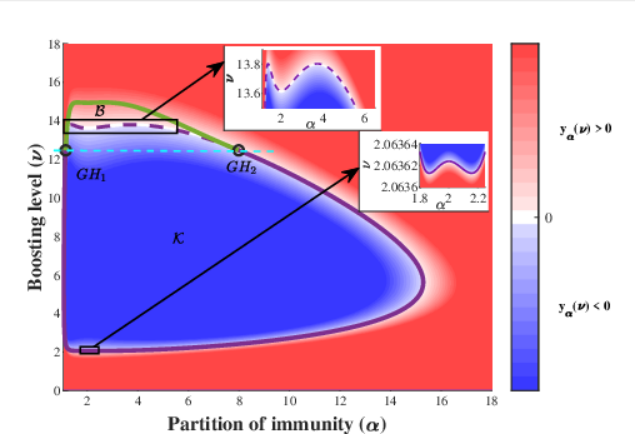
First, we recall that at $\mathcal{R}_{0}=1$ the transcritical bifurcation was shown to be solely of forward type. At the baseline parametrization $\mathcal{R}_{0}\approx 15.28$ and the endemic equilibrium is LAS but for the compact set $\mathcal{K}$ marked by blue. Note the symmetric presence of epidemic double bubbles around the baseline partitioning $\alpha=\omega=2$ in two boosting ranges, as highlighted in the insets of Figure 3(a). We recall two examples from [14], where the boosting values $\nu\approx 2.06362$ and $\nu\approx 13.7$ in these regions lead to the appearance of double bubbles, see Figure 4.

Figure 4: Baseline dynamics:

\xi=0

\rho\to\infty

. Bifurcation diagram w.r.t

\alpha

, with

\nu=2.06362

(left) and

\nu=13.7

(right). The depicted two bubbles of instability appear and disappear simultaneously. The later phenomenon is referred to as symmetric presence of bubbles.

For slightly larger boosting $\nu\approx 14$ , a bistable region $\mathcal{B}$ was observed where the EE is LAS together with a stable periodic orbit. The appearance of this bistable region is characterized by two generalized Hopf points $GH_{1}$ and $GH_{2}$ with identical $\nu$ coordinates.

Now, focusing on the current model and parametrization, first, we briefly study the direction of the transcritical bifurcation that is determined by the sign of $\Theta$ in Section 4.1, second, we analyze the stability of the EE through sign analysis of the Routh-Hurwitz criterion in Section 4.2. Then, we carry out numerical analysis of the bifurcations of the equilibrium branch and study how the bistable region is affected by the relative infectivity $\xi$ in Section 4.3.

4.1 Direction of the transcritical bifurcation

Substituting the baseline parametrization (24) into (18), we have that $\Theta>0$ is equivalent to

\nu\xi>\frac{1.00662\alpha}{\alpha-1}+\frac{0.125092}{\alpha}=:\mathbf{b}(\alpha)

with the corresponding zero contour displayed in Figure 5.

Clearly $\lim_{\alpha\to 1^{+}}\mathbf{b}(\alpha)=\infty$ and $\lim_{\alpha\to\infty}\mathbf{b}(\alpha)=1.0062$ , moreover, $\mathbf{b}(\alpha)$ is decreasing function of $\alpha$ . Consequently, the faster the transition from $W$ to $R$ , the smaller boosting coefficient $\nu$ is sufficient to activate backward transcritical bifurcation at $\mathcal{R}_{0}=1$ that is at $\beta=\gamma+\mu=17+1/80$ while keeping the relative infectivity $\xi$ fixed, or vice versa, smaller $\xi$ is required with keeping $\nu$ fixed. For example, assuming a moderate boosting coefficient, i.e. $\nu<3$ , and a relative infectivity $\xi\sim O(1)$ may very well result in a backward bifurcation for $\alpha\geq 1.5$ .

4.2 Stability switches of the EE

We constructed similar heatmaps to study the sign of $y_{\alpha}(\nu,\xi)$ , given by (23), for various values of relative infectivity $\xi\geq 0$ . Recall that $\rho=\gamma=17$ in our setting, thus, for $\xi=0$ we readily experience changes in the dynamics with respect to Figure 3. The instability set, marked as $\mathcal{K}_{\xi}$ to emphasize its dependence of $\xi$ , is somewhat similar but the regular shape resulting in simultaneous appearance of double-bubbles of instability is lost, see Figure 6. Note that in all figures that follow, $\mathcal{K}_{\xi}=\mathcal{K}$ for fixed $\xi$ . Now, the region around $\nu\approx 2.06$ displays much simpler behaviour. Additionally, for $\nu\approx 13.5$ , we still see bubbles, though without the symmetry they possess in the limit $\rho\to\infty$ .

By increasing $\xi\in(0,1)$ , we observe the following two phenomena. First, the shape of the $y_{\alpha}(\nu,\xi)=0$ curve that bounds the set $\mathcal{K}_{\xi}$ changes, therefore it influences the number of stability switches of the EE in the $(\alpha,\nu)$ plane. Second, the region $\mathcal{K}_{\xi}$ is shrinking and then disappearing, hence it results in the increase of local asymptotic stability region of the EE.

Dynamics of stability switches

For small $\xi$ , the Routh-Hurwitz criterion changes sign multiple times for boosting rates around $13.5$ as $\alpha$ is varied, suggesting the continued presence of multiple stability switches that is the aforementioned bubbles, see again Figures 6. As $\xi$ grows, the curve $y_{\nu}(\alpha,\xi)=0$ is deforming so that these double-bubbles disappear, as in Figure 7.

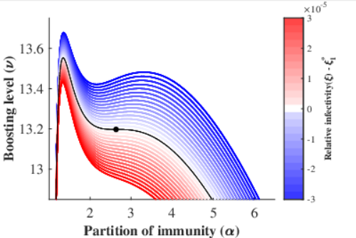
We localize the threshold value $\xi_{1}^{*}$ , at which the relevant change in the qualitative behavior of the curve $y_{\nu}(\alpha,\xi)=0$ occurs, as follows. In the region of interest ( $1<\alpha<6$ and $13<\nu$ ), the level curve $\alpha\mapsto\nu~\colon y_{\nu}(\alpha)=0$ , originally (when $\xi=0$ ), has two local maxima and one local minimum. As $\xi$ gets larger, the right maximum and the minimum collide, then disappear. Thus, the threshold scenario may be found by looking for $(\nu,\alpha,\xi)$ such that

\left[\begin{array}[]{c}~~y_{\nu}(\alpha,\xi)\\ \frac{\partial}{\partial\alpha}y_{\nu}(\alpha,\xi)\\ \frac{\partial^{2}}{\partial\alpha^{2}}y_{\nu}(\alpha,\xi)\\ \end{array}\right]=\left[\begin{array}[]{c}0\\ 0\\ 0\\ \end{array}\right],

yielding $\xi^{*}_{1}\approx 4.0098\times 10^{-5}$ . Figure 8 visualizes the transition in the qualitative behavior of the curve $y_{\nu}(\alpha,\xi)=0$ highlighting the one corresponding to the threshold value in black.

Shrinking of $\mathcal{K}_{\xi}$

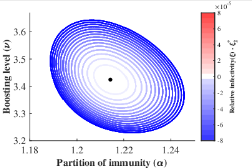
The second phenomenon we analyze is how the compact region of instability $\mathcal{K}_{\xi}$ shrinks and disappears as we increase $\xi$ , see Figure 9.

At the critical value $\xi^{*}_{2}$ , the region $\mathcal{K}_{\xi}$ has shrunk to a single point. Clearly, this is a zero of the Routh-Hurwitz criterion, moreover, it is a local minimum both with respect to $\alpha$ and $\nu$ . Hence, we look for $(\nu,\alpha,\xi)$ solving

\left[\begin{array}[]{c}~~y_{\nu}(\alpha,\xi)\\ \frac{\partial}{\partial\alpha}y_{\nu}(\alpha,\xi)\\ \frac{\partial}{\partial\nu}y_{\nu}(\alpha,\xi)\\ \end{array}\right]=\left[\begin{array}[]{c}0\\ 0\\ 0\\ \end{array}\right],

leading to $\xi^{*}_{2}\approx 9.19845\times 10^{-3}$ . For larger relative infectivity, i.e. $\xi>\xi_{2}^{*}$ , there is no region of instability, thus $\mathcal{K}_{\xi}=\emptyset$ , that is, the EE is LAS for all $(\alpha,\nu)$ . The localized transition is visualized in Figure 10.

Note that we did not investigate the dependence of these phenomena, and of the corresponding threshold values, on the other parameters fixed in (24).

4.3 Numerical bifurcation examples

In this section, we present numerical examples of one parameter $(\alpha)$ and two parameter $(\alpha,\nu)$ bifurcations of the endemic equilibria branch using MatCont [6]. An identical analysis we carried out in [14] for an SIRWS system, therefore here we show some interesting examples to highlight the dynamics in the presence of the $J$ compartment.

We briefly summarize the dynamics on the two parameter $(\alpha,\nu)$ bifurcation diagram when $\xi=10^{-5}<\xi_{1}^{*}$ , see Figure 11. The instability region $\mathcal{K}\,(\,=\mathcal{K}_{\xi}$ for fixed $\xi$ ) is enclosed by the purple-colored Hopf curve, which is continuous when supercritical (called $H_{-}$ ) and dashed when subcritical (called $H_{+}$ ).

The two generalized Hopf points $\mathrm{GH}_{1}$ and $\mathrm{GH}_{2}$ , mark the parameter values where the Hopf bifurcation changes from supercritical to subcritical. Note that these points now possess different $\nu$ coordinates as opposed to the limiting case in Figure 3. The branch of the limit points of periodic cycles appears in green, which together with the dashed purple curve $H_{+}$ enclose a bistability region $\mathcal{B}$ , where there exists a stable periodic solution alongside the LAS endemic equilibrium.

Let us now examine the bifurcation diagram in more detail over regions, characterized by various levels of boosting rate $\nu$ , where the dynamics is similar, see Figure 12 for such partition and Table 2 for the critical boosting values.

$\nu^{*}_{1}$	$\nu^{*}_{GH_{2}}$	$\nu^{*}_{GH_{1}}$	$\nu^{*}_{2}$	$\nu^{*}_{3}$	$\nu^{*}_{4}$	$\nu^{*}_{5}$
$2.0248$	$11.9494$	$12.3922$	$13.42$	$13.48$	$13.6785$	$14.7675$

Table 2: Approximate critical boosting values

(\nu^{*}_{k})

using the parametrization (24) and fixing

\xi=10^{-5}

as in Figure 12.

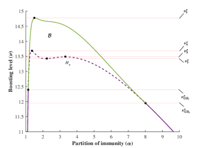
In all bifurcation plots that follow, the endemic equilibria branch (particularly the $I$ and $J$ components) is marked with black curve, solid when LAS and dashed when unstable. Red and blue curves represent branches of stable and unstable limit cycles, respectively, and Hopf bifurcation points are marked with purple dots.

Below we describe the situation for various ranges of $\nu$ .

Boosting: $\nu<\nu_{1}^{*}$

The system has a stable point attractor for all $\alpha>1$ .

Boosting: $\nu_{1}^{}<\nu<\nu_{GH_{2}}^{}$

There are two supercritical Hopf bifurcation points on the endemic equilibria branch, see the lower inset in Figure 7(a). Continuation of limit cycles with respect to $\alpha$ starting from two Hopf bifurcation points, $\mathrm{H}_{1}$ and $\mathrm{H}_{2}$ , forms an endemic bubble, where the two branches of stable limit cycles coincide, see Figure 13.

Boosting: $\nu_{GH_{2}}^{}<\nu<\nu_{GH_{1}}^{}$

As $\nu$ continues to grow in the two-parameter plane in Figure 12 the generalized Hopf point $\mathrm{GH}_{2}$ appears, which separates branches of sub- and supercritical Hopf bifurcations. The stable limit cycles survive when we enter the region $\mathcal{B}$ . Crossing the subcritical Hopf boundary $H_{+}$ leads to an additional unstable cycle inside the first one, while the equilibrium regains its stability. Two cycles of opposite stability exist inside the bistable region $\mathcal{B}$ and disappear at the green curve.

Let us fix $\nu$ in this boosting region. Then Figure 14 shows a typical bifurcation with respect to $\alpha$ . Observe here the small $\alpha$ -parameter range of bistability where the EE and the larger amplitude periodic solution are both stable. The points marked with green circle are limit points of periodic orbits. The stable and unstable cycles collide and disappear on the green curve in Figure 12, corresponding to a fold bifurcation of cycles.

Boosting: $\nu_{GH_{1}}^{}<\nu<\nu_{2}^{}$

In this boosting range, as we passed $\mathrm{GH}_{1}$ , the Hopf curve changed to subcritical. Figure 15 confirms the appearance of two subcritical Hopf bifurcations on the equilibria branch, then again a fold bifurcation of cycles occurs (marked with green circles), resulting in two small $\alpha$ -parameter intervals of bistability.

Boosting: $\nu_{2}^{}<\nu<\nu_{3}^{}$

In this region, we can observe how the shape of the Hopf curve $H_{+}$ that bounds the set $\mathcal{K}_{\xi}$ influences the number of stability switches of the EE. In Figure 16, the bifurcation diagram shows the existence of four subcritical Hopf bifurcation points. Here, a small bubble appears inside the region of stable oscillations, which leads to an additional bistable region compared to the previous case. When we increase the boosting parameter but still being in this region, then the Hopf points $\mathrm{H}_{1}$ and $\mathrm{H}_{2}$ as well as $\mathrm{H}_{3}$ and $\mathrm{H}_{4}$ move closer to each other, resulting in larger bistability regions, see also Figure 12.

Boosting: $\nu_{3}^{}<\nu<\nu_{4}^{}$

Here, the two Hopf points $\mathrm{H}_{3}$ and $\mathrm{H}_{4}$ seen in the region before collided and disappeared, see Figure 17. The dynamics is similar to Figure 15 but the boosting values in this range lead to much larger bistability regions.

Boosting: $\nu_{4}^{}<\nu<\nu_{5}^{}$

Although, we are in the bistability region in the two-parameter bifurcation plot, we do not cross any Hopf curve, hence the numerical continuation method finds a stable equilibrium branch, see Fig 18.

Boosting: $\nu_{5}^{*}<\nu$

The system has a stable point attractor for all $\alpha>1$ .

Shrinking of the bistability region

In Section 4.2 we analyzed the shrinking of the instability region $\mathcal{K}_{\xi}$ as $\xi$ increases. As a consequence, the bistability region $\mathcal{B}$ becomes smaller, the generalized Hopf points move towards each other, then collide and disappear as illustrated in Figure 19. We did not localize further the threshold value $\xi^{*}_{\footnotesize\mathcal{B}}\in(8.3,8.4)\times 10^{-3}$ at which this region disappears.

5 Conclusion

In this paper, we carried out combined analytical and numerical investigations of the $SIRWJS$ system with the presence of secondary infections and potentially asymmetric partitioning of the immune boosting period. As the model population is assumed to be constant, the system is inherently four dimensional resulting in rather complicated formulae describing the equilibria and their stability. The analysis presented in this manuscript is giving us novel insights into this complexity and a better understanding of the dynamics. We concluded an exact condition in the form of $\Theta$ determining the direction of the bifurcation at $\mathcal{R}_{0}=1$ , and showed that backward bifurcation is possible. For $\mathcal{R}_{0}>1$ , we derived a numerically tractable Routh-Hurwitz stability criterion and carried out its sign analysis together with numerical continuation techniques. We observed rich and interesting dynamics in the $(\nu,\alpha,\xi)$ -space that is varying the immune boosting rate, the partitioning of the boosting period, and the relative infectivity of secondary infections, where other disease parameters were set according to pertussis parameter values taken from the literature. Nevertheless, we note that most of the mathematically appealing phenomena occur for rather large boosting rate ( $\nu$ ) and very small relative infectivity ( $\xi$ ).

Overall, our results highlight the potential complexities generated by the combination of waning and boosting of immunity, which makes the prediction of the long term dynamics rather challenging for diseases when these processes are relevant, such as COVID-19 or pertussis.

Acknowledgement

This research was completed in the National Laboratory for Health Security RRF-2.3.1-21-2022-00006. Additionally, the work was supported by the Ministry of Innovation and Technology of Hungary from the National Research, Development and Innovation Fund project no. TKP2021-NVA-09. In addition, F.B. and G.R. were supported by NKFIH grant numbers FK 138924, KKP 129877. M.P. was also supported by the Hungarian Scientific Research Fund grant numbers K129322 and SNN125119; F.B. was also supported by UNKP-22-5 and the Bolyai scholarship of the Hungarian Academy of Sciences.

References

[1] M.V. Barbarossa, G. Röst, Immuno-epidemiology of a population structured by immune status: a mathematical study of waning immunity and immune system boosting, J. Math. Biol. 71 (6) (2015) 1737–1770.
https://doi.org/10.1007/s00285-015-0880-5.
https://pubmed.ncbi.nlm.nih.gov/25833186.
https://mathscinet.ams.org/mathscinet-getitem?mr=3419906.
[2] R.M. Carlsson, L.M. Childs, Z. Feng, J.W. Glasser, J.M. Heffernan, J. Li, G. Röst, Modeling the waning and boosting of immunity from infection or vaccination, J. Theor. Biol. 497 (2020) 110265.
https://doi.org/10.1016/j.jtbi.2020.110265.
https://pubmed.ncbi.nlm.nih.gov/32272134.
[3] C. Castillo-Chavez, B. Song, Dynamical models of tuberculosis and their applications, Math. Biosci. Eng. 1 (2) (2004) 361–404.
https://doi.org/10.3934/mbe.2004.1.361.
https://pubmed.ncbi.nlm.nih.gov/20369977.
https://mathscinet.ams.org/mathscinet-getitem?mr=2130673.
[4] L. Childs, D.W. Dick, Z. Feng, J.M. Heffernan, J. Li, G. Röst, Modeling waning and boosting of COVID-19 in Canada with vaccination, Epidemics, 39 (2002) 100583. https://doi.org/10.1016/j.epidem.2022.100583.
https://pubmed.ncbi.nlm.nih.gov/35665614.
[5] M.P. Dafilis, F. Frascoli, J.G. Wood, J.M. McCaw, The influence of increasing life expectancy on the dynamics of SIRS systems with immune boosting, The ANZIAM Journal 54 (1-2) (2012) 50–63.
https://doi.org/10.1017/S1446181113000023.
https://mathscinet.ams.org/mathscinet-getitem?mr=3066288.
[6] A. Dhooge, W. Govaerts, Y.A. Kuznetsov, MATCONT: a Matlab package for numerical bifurcation analysis of ODEs, SIGSAM Bull. 38 (1) (2004) 21–22.
https://doi.org/10.1145/980175.980184.
https://mathscinet.ams.org/mathscinet-getitem?mr=2000880.
[7] O. Diekmann, J.A.P. Heesterbeek, M.G. Roberts, The construction of next-generation matrices for compartmental epidemic models, J. R. Soc. Interface 7 (47) (2010) 873–885.
https://doi.org/10.1098/rsif.2009.0386.
https://pubmed.ncbi.nlm.nih.gov/19892718.
[8] J. Heidecke, M.V. Barbarossa, When Ideas Go Viral—Complex Bifurcations in a Two-Stage Transmission Model, In: Mondaini, R.P. (eds) Trends in Biomathematics: Chaos and Control in Epidemics, Ecosystems, and Cells. BIOMAT 2020. Springer, Cham.
https://doi.org/10.1007/978-3-030-73241-7_14.
https://mathscinet.ams.org/mathscinet-getitem?mr=4306495.
[9] G. Katriel, The dynamics of two-stage contagion, Chaos, Solitons & Fractals: X, 2 (2019) 100010.
https://doi.org/10.1016/j.csfx.2019.100010.
[10] J.S. Lavine, A.A. King, O.N. Bjørnstad, Natural immune boosting in pertussis dynamics and the potential for long-term vaccine failure, PNAS 108 (17) (2011) 7259–7264.
https://doi.org/10.1073/pnas.1014394108.
https://pubmed.ncbi.nlm.nih.gov/21422281.
[11] T. Leung, P.T. Campbell, B.D. Hughes, F. Frascoli, J.M. McCaw, Infection-acquired versus vaccine-acquired immunity in an SIRWS model, Infect. Dis. Model. 3 (2018) 118–135.
https://doi.org/10.1016/j.idm.2018.06.002.
https://pubmed.ncbi.nlm.nih.gov/30839933.
[12] M. Liu, E. Liz, G. Röst, Endemic bubbles generated by delayed behavioral response: global stability and bifurcation switches in an SIS model, SIAM J. Appl. Math. 75 (1) (2015) 75–91.
https://doi.org/10.1137/140972652.
https://mathscinet.ams.org/mathscinet-getitem?mr=3299143.
[13] J.D. Murray, Mathematical Biology: I. An Introduction. Interdisciplinary Applied Mathematics, 17, Springer-Verlag, New York, New York, 2002.
https://doi.org/10.1007/b98868.
https://mathscinet.ams.org/mathscinet-getitem?mr=1908418.
[14] R. Opoku-Sarkodie, F.A. Bartha, M. Polner, G. Röst, Dynamics of an SIRWS model with waning of immunity and varying immune boosting, J. Biol. Dyn. 16 (1) (2022) 596–618.
https://doi.org/10.1080/17513758.2022.2109766.
https://pubmed.ncbi.nlm.nih.gov/35943129.
https://mathscinet.ams.org/mathscinet-getitem?mr=4466048.
[15] E.J. Routh, A treatise on the Stability of a given state of motion: particularly steady motion, Macmillan and Co., London, 1877.
[16] L.F. Strube, M. Walton, L.M. Childs, Role of repeat infection in the dynamics of a simple model of waning and boosting immunity, J. Biol. Syst. 29 (2) (2021) 1–22.
https://doi.org/10.1142/S0218339021400076.
https://mathscinet.ams.org/mathscinet-getitem?mr=4274350.
[17] Computer Algebra Codes, Github, 2023.
https://github.com/epidelay/waning-boosting-epidemiological-models.

Bifurcation analysis of waning-boosting epidemiological models with repeat infections and varying immunity periods

Abstract

Keywords:

1 Introduction

2 Description of the SIRWJS model: a compartmental model with waning and boosting, where secondary exposure can make the host infective

3 Equilibria and stability analysis

Lemma 1.

Proof.

3.1 Disease free equilibrium

3.2 Existence of non-trivial equilibria

Theorem 1.

Remark

Proof.

3.3 Transcritical bifurcation at ℛ0=1\mathcal{R}_{0}=1

Theorem 2.

Proof.

3.4 Case ξ=0\xi=0

3.5 Stability of the endemic equilibrium for ℛ0>1\mathcal{R}_{0}>1

Theorem 3 (Routh-Hurwitz).

4 Exploring bifurcations using numerics

4.1 Direction of the transcritical bifurcation

4.2 Stability switches of the EE

Dynamics of stability switches

Shrinking of 𝒦ξ\mathcal{K}_{\xi}

4.3 Numerical bifurcation examples

Boosting: ν<ν1∗\nu<\nu_{1}^{*}

Boosting: ν1∗<ν<νG​H2∗\nu_{1}^{*}<\nu<\nu_{GH_{2}}^{*}

Boosting: νG​H2∗<ν<νG​H1∗\nu_{GH_{2}}^{*}<\nu<\nu_{GH_{1}}^{*}

Boosting: νG​H1∗<ν<ν2∗\nu_{GH_{1}}^{*}<\nu<\nu_{2}^{*}

Boosting: ν2∗<ν<ν3∗\nu_{2}^{*}<\nu<\nu_{3}^{*}

Boosting: ν3∗<ν<ν4∗\nu_{3}^{*}<\nu<\nu_{4}^{*}

Boosting: ν4∗<ν<ν5∗\nu_{4}^{*}<\nu<\nu_{5}^{*}

Boosting: ν5∗<ν\nu_{5}^{*}<\nu

Shrinking of the bistability region

5 Conclusion

Acknowledgement

References

3.3 Transcritical bifurcation at $\mathcal{R}_{0}=1$

3.4 Case $\xi=0$

3.5 Stability of the endemic equilibrium for $\mathcal{R}_{0}>1$

Shrinking of $\mathcal{K}_{\xi}$

Boosting: $\nu<\nu_{1}^{*}$

Boosting: $\nu_{1}^{}<\nu<\nu_{GH_{2}}^{}$

Boosting: $\nu_{GH_{2}}^{}<\nu<\nu_{GH_{1}}^{}$

Boosting: $\nu_{GH_{1}}^{}<\nu<\nu_{2}^{}$

Boosting: $\nu_{2}^{}<\nu<\nu_{3}^{}$

Boosting: $\nu_{3}^{}<\nu<\nu_{4}^{}$

Boosting: $\nu_{4}^{}<\nu<\nu_{5}^{}$

Boosting: $\nu_{5}^{*}<\nu$