DFT+U Type Strong Correlation Functional Derived from Multiconfigurational Wavefunction TheoryPreprint: AIP/123-QED

Kohn-Sham density functional theory (DFT) introduces electron correlation into a mean-field model of electronic structure. Standard DFT approximations do this imperfectly, leading to zero-sum tradeoffs between over-delocalization of charge and spin, and understimation of electron correlation.Janesko2021; Bryenton2022 Figure 1 shows an example of these tradeoffs, comparing the delocalization error in fractionally charged Fe^(3+δ)+, to the spin splitting error in spin-crossover complexFinney2022 [Fe(CO)₆]²⁺. (Computational details are in the Supplemental Material). DFT+U and hybrid DFT approximations that accurately model the spin splitting introduce large delocalization errors, and vice versa. Because of these tradeoffs, choosing (or tuning) a DFT approximation to model one property often degrades accuracy for other properties.Hughes2010

For decades, the DFT community has explored methods to go beyond these tradeoffs. Many of these methods incorporate localized single-particle states to capture aspects of delocalization & correlation.Janesko2021 Examples include projection of the exchange hole onto a localized model,Becke2005 comparisons of localized vs. delocalized exchange holes,Perdew2008; Haasler2020 and projections of the reference system wavefunction onto localized orbitalets,Su2018 atomic states,Bajaj2017 or localized states at each point in space.Verma2019 Determining appropriate functional forms remains a challenge. For example, the form of our nondynamical correlation model was based on educated guesses about opposite-spin correlation.Ramos2020 Recent extended DFT+U methods employ multi-parameter fits to recover the flat-plane condition.Bajaj2017; Bajaj2019; Bajaj2022; Burgess2023 This ambiguity can be contrasted with the generalized range-separated approach to correcting DFT. In this approach, part of the electron-electron interaction is reintroduced into the reference system, the reference system wavefunction is treated with a multideterminant approximation, and a modified exchange-correlation (XC) density functional accounts for the remaining electron-electron interactions.Savin1988; Autschbach2014 The functional forms of generalized range-separated approaches are unambiguous, free of double-counting, and can in principle be systematically improved to the exact answer.

This work present a DFT+U-type functional for strong correlation, derived directly from a multiconfigurational wavefunction. The formalism is our further generalizationJanesko2022a of the generalized range-separated approach. The reference system’s correlated wavefunction is modeled using ideas from valence bond approaches.Beran2005 The XC functional is modifiedJanesko2022b following the Perdew-Zunger self-interaction correction (PZSIC)Perdew1981 to eliminate double-counting.

Our approach is based on the simplified rotationally averaged formulation of DFT+U.Dudarev1998; Cococcioni2005; Kulik2015 In this approach, one projects the reference system wavefunction onto $N_{proj}=N_{shell}L_{shell}$ orthonormal one-electron states $\{\tilde{\chi}_{Ip}\}$ localized at $N_{shell}$ atomic shells $I$, and introduces an energetic penalty $U_{eff}$ for fractional occupation.

${\tilde{n}}^{I\sigma}_{pq}=\sum_{i}\left<\psi_{i\sigma}|\tilde{\chi}_{Ip}\right>\left<\tilde{\chi}_{Iq}|\psi_{i\sigma}\right>$ is the $\sigma$-spin projected density matrix obtained by projecting the reference system single-determinant wavefunction $\left|\Phi_{0}\right>$, built from occupied spinorbitals $\{\psi_{i\sigma}\}$, onto $\{\tilde{\chi}_{Ip}\}$. $n_{Ip\sigma}$ is the $p$th eigenvalue of the $L_{shell}xL_{shell}$ block ${\bf{\tilde{n}}}^{I\sigma}$, corresponding to eigenfunction $\chi_{Ip\sigma}$. (We assume that ${\bf{{\tilde{n}}}}$ is block-diagonal in spin $\sigma$ and shells $I$.) Extended DFT+U approaches add terms such as $n_{pq}^{I\uparrow}n_{qp}^{I\downarrow}$ to model strong correlation.Bajaj2017; Bajaj2019; Bajaj2022; Burgess2023

The present work extends our rederivation of DFT+U,Janesko2022b which builds on the connections between DFT+U and hybrid DFT.Andriotis2010; Ivady2014; Agapito2015 Consider an $N$-electron system in external potential $\hat{V}_{ext}$ and a reference system of $N$ noninteracting electrons whose single-determinant ground state wavefunction $\left|\Phi_{0}\right>$ yields density $\rho(\vec{r})=\sum_{i\sigma}|\psi_{i\sigma}(\vec{r})|^{2}$. The ground-state energy is $E_{DFT}=\left<\Phi_{0}|\hat{T}+\hat{V}_{ext}|\Phi_{0}\right>+J[\rho]+E_{XC}[\rho_{\uparrow},\rho_{\downarrow}]$. $\hat{T}$ and $\hat{V}_{ext}$ are kinetic and external potential operators. $J[\rho]$ is the mean-field Hartree energy corresponding to density $\rho$. The “exact” exchange piece of $E_{XC}$, $E_{X}^{ex}[\rho]=\left<\Phi_{0}|\hat{V}_{ee}|\Phi_{0}\right>-J[\rho]$, is defined in terms of the electron-electron interaction operator $\hat{V}_{ee}=\sum_{i>j}|\vec{r}_{i}-\vec{r}_{j}|^{-1}$ The Hohenberg-Kohn theorems ensure that minimizing $E_{DFT}$ using the exact $E_{XC}[\rho_{\uparrow},\rho_{\downarrow}]$ recovers the exact ground-state density and energy of the real system.

To rederive DFT+U, we project $\hat{V}_{ee}$ onto the states $\{\chi_{Ip\sigma}\}$ introduced above:

$J_{I}=\left<\chi_{Ip\sigma}(1)\chi_{Ip\sigma}(2)||\vec{r}_{1}-\vec{r}_{2}|^{-1}|\chi_{Ip\sigma}(1)\chi_{Ip\sigma}(2)\right>$ is the self-Hartree interaction of an electron in state $\chi_{Ip\sigma}$. The reference system Hamiltonian becomes $\hat{T}+\hat{V}_{ext}+\hat{V}^{P}_{ee}$. Because $\{\chi_{Ip\sigma}\}$ are eigenfunctions of the projected one-particle density matrix corresponding to $\left|\Phi_{0}\right>$, the projection $\sum_{i}\left<\Phi_{0}|\chi_{Ip\sigma}(i)\right>\left<\chi_{Iq\sigma}(i)|\Phi_{0}\right>=n_{Ip\sigma}\delta_{pq}$. This ensures that the expectation value of the projected electron-electron interaction $\left<\Phi_{0}|\hat{V}_{ee}^{P}|\Phi_{0}\right>$ becomes $\sum_{I}(J_{I}/2)\sum_{p\sigma}(n_{Ip\sigma}^{2}-n_{Ip\sigma}^{2})$, which equals zero. Thus, $\hat{V}^{P}_{ee}$ introduces only electron self-interaction into the reference system. The reference system’s exact ground-state wavefunction is a single Slater determinant, and the Hohenberg-Kohn theorems ensure the existence of an exact projected Hartree-exchange-correlation density functional. We define the projected Hartree functional as $J^{P}[\rho]=J[\rho]-\sum_{Ip\sigma}J_{I}n_{Ip\sigma}^{2}$. Inspired by the PZSIC,Perdew1981 we model the projected XC functional by passing projected single-particle densities $n_{Ip\sigma}|\chi_{Ip\sigma}(\vec{r})|^{2}$ to the XC functional, giving $E_{XC}^{P}[\rho_{\uparrow},\rho_{\downarrow}]=E_{XC}[\rho_{\uparrow},\rho_{\downarrow}]-\sum_{Ip\sigma}E_{XC}[n_{Ip\sigma}|\chi_{Ip\sigma}|^{2},0]$. The ground-state energy becomes

(The projected Hartree energy is included in the Hartree energy in $E_{DFT}$.) Approximating the double-counting correction as $E_{XC}[n_{Ip\sigma}|\chi_{Ip\sigma}|^{2},0]\simeq-c_{1}n_{Ip\sigma}-c_{2}n^{2}_{Ip\sigma}$, constrained to obey $c_{1}=(J_{I}-c_{2})$, makes eq 3 recover eq 1. The resulting $U_{eff}=(J_{I}-c_{2})$ has a transparent dependence on the choice of projection statesAndriotis2010 and approximate XC functional. The exact XC functional, or any functional which is exact for one-electron systems, correctly gives $U_{eff}=0$.

We next add to $\hat{V}_{ee}^{P}$ the opposite-spin interactions $\sum_{i>j}\sum_{Ip}\sum_{\sigma^{\prime}\neq\sigma}\left|\chi_{Ip\sigma}(i)\chi_{Ip\sigma^{\prime}}(j)\right>J_{I}\left<\chi_{Ip\sigma}(i)\chi_{Ip\sigma^{\prime}}(j)\right|$. (We assume negligible spin contamination of $\tilde{{\bf{n}}}^{I\sigma}$ so that each eigenfunction $\chi_{Ip\uparrow}$ corresponds to one $\chi_{Ip\downarrow}$.) The projected Hartree and XC functionals become $J^{P}[\rho]=J[\rho]-\sum_{Ip\sigma\sigma^{\prime}}J_{I}n_{Ip\sigma}n_{Ip\sigma^{\prime}}$ and $E_{XC}^{P}[\rho_{\uparrow},\rho_{\downarrow}]=E_{XC}[\rho_{\uparrow},\rho_{\downarrow}]-\sum_{Ip}E_{XC}[n_{Ip\uparrow}|\chi_{Ip\uparrow}|^{2},n_{Ip\downarrow}|\chi_{Ip\downarrow}|^{2}]$. $\left<\Phi_{0}|\hat{V}^{P}_{ee}|\Phi_{0}\right>$ is no longer zero and the reference system’s exact ground-state wavefunction is no longer a single Slater determinant.

We approximate this correlated wavefunction using ideas from valence bond theory.Beran2005 We perform a unitary transform of the occupied orbitals $\{\psi_{i\sigma}\}$ in $\left|\Phi_{0}\right>$, so that each $\chi_{Ip\sigma}$ has a nonzero projection onto only one transformed occupied orbital denoted $\phi^{(o)}_{Ip\sigma}$. The unitary transform does not change the projection of $\left|\Phi_{0}\right>$ onto state $\chi_{Ip\sigma}$, ensuring $|\left<\chi_{Ip\sigma}|\phi^{(o)}_{I^{\prime}p^{\prime}\sigma^{\prime}}\right>|^{2}=n_{Ip\sigma}\delta_{II^{\prime}}\delta_{pp^{\prime}}\delta_{\sigma\sigma^{\prime}}$. We perform a corresponding transform of the unoccupied (virtual) Kohn-Sham orbitals $\{\psi_{a\sigma}\}$, such that each $\chi_{Ip\sigma}$ has a nonzero projection onto only one transformed virtual orbital $\phi^{(v)}_{Ip\sigma}$. Orthogonality of occupied-virtual spaces and completeness of the occupied+virtual space ensures $|\left<\chi_{Ip\sigma}|\phi^{(v)}_{Ip\sigma}\right>|^{2}=1-n_{Ip\sigma}$. (A key to our approach is that these transforms can be either approximated, or evaluated explicitly.) We approximate the reference system’s wavefunction as a superposition of $\left|\Phi_{0}\right>$ and the $N_{proj}$ “doubly excited” Slater determinants $\left|\Phi_{Ipo}^{Ipv}\right>$ in which $\phi^{(o)}_{Ip\uparrow}$ is replaced by $\phi^{(v)}_{Ip\uparrow}$ and $\phi^{(o)}_{Ip\downarrow}$ is replaced by $\phi^{(v)}_{Ip\downarrow}$. $\hat{V}^{P}_{ee}$ does not include electron-electron interactions between the $N_{proj}$ different states $p$. (These interactions are treated by the projected Hartree-exchange-correlation functional.) Accordingly, the reference system’s configuration interaction (CI) Hamiltonian is block-diagonalized into $N_{proj}$ $2x2$ matrices

Here $\left<\Phi_{0}|\hat{V}_{ee}^{P}|\Phi_{Ipo}^{Ipv}\right>$ $=\left<\phi^{(o)}_{Ip\uparrow}\phi^{(o)}_{Ip\downarrow}|\hat{V}^{P}_{ee}|{\phi^{(v)}_{Ip\uparrow}\phi^{(v)}_{Ip\downarrow}}\right>$ equal $J_{I}\sqrt{n_{Ip\uparrow}(1-n_{Ip\uparrow})n_{Ip\sigma^{\prime}}(1-n_{Ip\downarrow})}$. The diagonal elements introduce the unitless promotion energy $\Delta_{Ip}$=$J_{I}^{-1}\left(\left<\Phi_{Ipo}^{Ipv}|\hat{H}_{0}|\Phi_{Ipo}^{Ipv}\right>-\left<\Phi_{0}|\hat{H}_{0}|\Phi_{0}\right>\right)$, where $\hat{H}_{0}$ is the Hamiltonian of the projected-interacting reference system. $\Delta_{Ip}\geq 0$, otherwise $\left|\Phi_{0}\right>$ would not be the reference system’s lowest-energy single Slater determinant wavefunction. The reference system’s correlation energy is the sum of the lower eigenvalues of these $2x2$ Hamiltonian blocks. The final energy is

Eq 7 does not double-count exchange or correlation, just as the PZSIC does not double-count exchange or correlation. Eq 7 is reminiscent of the forms of other extended DFT+U approximations.Bajaj2017; Bajaj2019; Bajaj2022; Burgess2023

We may evaluate eq 7 exactly for asymptotically stretched singlet hydrogen molecule H₂ in an orthonormal minimal basis set of functions $\chi_{A},\chi_{B}$ localized to atoms A and B. We construct orthonormal spinorbitals $\psi_{1\sigma}=c_{A}\chi_{A\sigma}+(1-c_{A}^{2})^{1/2}\chi_{B\sigma}$, $\psi_{2\sigma}=(1-c_{A}^{2})^{1/2}\chi_{A\sigma}-c_{A}\chi_{B\sigma}$ . The spin-symmetry-unrestricted mean-field state $\left|\Phi_{0}\right>=\left|\psi_{1\uparrow}\psi_{2\downarrow}\right>$ places $n_{A\uparrow}=|c_{A}|^{2}$ $\uparrow$-spin electrons and $n_{A\downarrow}=1-n_{A\uparrow}$ $\downarrow$-spin electrons on atom A. For any $n_{A\uparrow}$, configurations $\left|\psi_{1\uparrow}\psi_{2\downarrow}\right>$ and $\left|\psi_{2\uparrow}\psi_{1\downarrow}\right>$ are degenerate. For the exact ground state, all configurations with $0\leq n_{A\uparrow}\leq 1$ are degenerate, the so-called fractional spin line (FSL).Yang2000 Unrestricted Hartree-Fock calculations give the exact energy at $n_{A\uparrow}=0$ or 1, and insufficiently negative energies at intermediate $n_{A\uparrow}$ (fractional spin error). To evaluate eq 7, we project the electron-electron interaction operator onto $N_{shell}=2$ shells each with $L_{shell}=1$, i.e., onto $\chi_{A}$ and $\chi_{B}$. Because $L_{shell}=1$, the projected density matrix eigenfunction $\chi_{I=1,p=1,\sigma}$ introduced above is $\chi_{A\sigma}$. The projected XC energy $E_{XC}^{P}=E_{XC}[\rho]-\sum_{S=A,B}E_{XC}[n_{S\uparrow}|\chi_{S}|^{2},n_{S\downarrow}|\chi_{S}|^{2}]$ is zero. Because there is only one occupied and one virtual orbital of each spin, the projected states in eq DFT+U Type Strong Correlation Functional Derived from Multiconfigurational Wavefunction Theory become $\phi^{(o)}_{I=1,p=1,\sigma}=\psi_{1\sigma}$ and $\phi^{(v)}_{I=1,p=1,\sigma}=\psi_{2\sigma}$, such that $\left|\Phi_{Ipo}^{Ipv}\right>=\left|\psi_{2\uparrow}\psi_{1\downarrow}\right>$. Because $\left|\psi_{2\uparrow}\psi_{1\downarrow}\right>$ and $\left|\psi_{1\uparrow}\psi_{2\downarrow}\right>$ are degenerate, $\left|\Phi_{0}\right>$ and $\left|\Phi_{Ipo}^{Ipv}\right>$ are degenerate and $\Delta$=0. Eq DFT+U Type Strong Correlation Functional Derived from Multiconfigurational Wavefunction Theory with $\Delta=0$ becomes the full configuration interaction (FCI) Hamiltonian in this minimal basis, and eq 7 is the exact FCI ground-state energy.

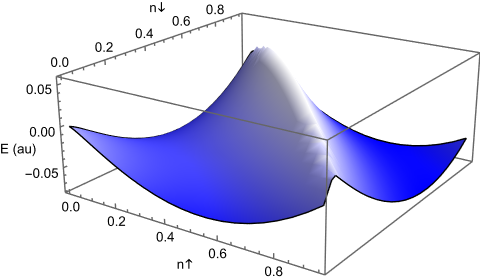
Eq 7 can be evaluated for the entire “flat-plane condition”. We follow ref 28, treating an integer number of electrons distributed across asymptotically separated hydrogen nuclei such that each atom has average populations $0\leq n_{\uparrow},n_{\downarrow}\leq 1$. The exact energy of the real system is (to within infintesimal error) a sum of subsystem energies $E[n_{\uparrow},n_{\downarrow}]$, where $E[n_{\uparrow},n_{\downarrow}]$ is composed of two flat planes intersecting at the FSL.MoriSanchez2014; Kong2022 Figure 2 illustrates eq 3 and 7 for this system. Calculations use the STO-6G basis set, the Perdew-Burke-Ernzerhof (PBE) XC functional,Perdew1996 and choose the projection state as the STO-6G basis function for hydrogen atom. PySCF codeSun2020 for the calculations in Figure 2 is provided as Supplementary Information. We consider eq 7 with $\Delta=|n_{\uparrow}+n_{\downarrow}-1|\equiv\Delta_{FP}$. These calculations recover the exact flat-plane energy,MoriSanchez2014 including constant energy along the FSL, zero correlation energy for the minimal-basis closed-shell anion $n_{\uparrow}=n_{\downarrow}=1$, and a discontinuity when crossing the FSL. This approach is nearly exact for other atoms and larger basis sets (Supplementary Information). The form of $\Delta_{FP}$ may be rationalized as follows. When $n=n_{\uparrow}+n_{\downarrow}$ is 1, $\Delta=0$ as derived above. As $n$ approaches 0 or 2, the Hartree-Fock energy becomes an increasingly good approximation to FCI. the FCI wavefunction is increasingly dominated by a single determinant, thus $\Delta$ must increase. The correction to $E_{DFT}$, plotted as a function of $n_{\uparrow},n_{\downarrow}$, is qualitatively similar to other extended DFT+U methods (Supplementary Information).

Eq 7 can be applied to more realistic systems. Table 1 shows the predicted spin splitting of four iron(II) spin-crossover (SCO) complexes. Figure 3 illustrates delocalization error, computed as the energy to ionize a pair of distant high-spin Fe³⁺ ions to yield (Fe${}^{(3+\delta)+}\ldots$Fe^(4-δ)+), relative to the energy at $\delta=0$. Figure 1 plots the predicted spin splitting of [Fe(CO)₆]²⁺ versus the delocalization error at $\delta=1/2$. Eq 3 and eq 7 both include full exact exchange in the projected states, and both give low delocalization error in Figure 3. However, eq 3 gives underestimated spin splittings in Table 1, and eq 7 with $\Delta_{FP}$ The correlation terms in eq 7 correct these underestimations. While $\Delta_{FP}$ is exact for the flat-plane condition, it is insufficiently robust for practical calculations (Supplementary Information) and underestimates the spin splittings in Table 1. Choosing constant $\Delta=0.35$ accurately models spin splittings. More importantly, Figure 1 shows that different choices of $\Delta$ all give negligible delocalization error for Fe³⁺ ionization. Eq 7 provides beyond-zero-sum performance at mean-field cost.

The results presented here provide a new perspective on beyond-zero-sum DFT. By projecting the electron-electron interaction onto specific atomic states, we can introduce a controlled degree of electron correlation into the reference system. Exact or nearly exact treatments of this strong correlation may be rigorously embedded into DFT. This general derivation may be extended to other single-particle states and more sophisticated approximations for the promotion energy $\Delta$, providing new insight into DFT-based treatments of strong correlation.Bajaj2017; Bajaj2019; Bajaj2022; Burgess2023

Supplemental Materials: DFT+U Type Strong Correlation Functional Derived from Multiconfigurational Wavefunction Theory

References

- (1) B. G. Janesko, Replacing hybrid density functional theory: motivation and recent advances, Chem. Soc. Rev. 50, 8470 (2021).
- (2) K. R. Bryenton, A. A. Adeleke, S. G. Dale, and E. R. Johnson, Delocalization error: The greatest outstanding challenge in density-functional theory, WIREs Computational Molecular Science 13 (2022).
- (3) B. A. Finney, S. R. Chowdhury, C. Kirkvold, and B. Vlaisavljevich, CASPT2 molecular geometries of Fe(II) spin-crossover complexes, Phys. Chem. Chem. Phys. 24, 1390 (2022).
- (4) T. F. Hughes and R. A. Friesner, Correcting systematic errors in DFT spin-splitting energetics for transition metal complexes, J. Chem. Theory Comput. 7, 19 (2010).
- (5) A. D. Becke, Real-space post-Hartree-Fock correlation models, J. Chem. Phys. 122, 064101 (2005).
- (6) J. P. Perdew, V. N. Staroverov, J. Tao, and G. E. Scuseria, Density functional with full exact exchange, balanced nonlocality of correlation, and constraint satisfaction, Phys. Rev. A 78, 052513 (2008).
- (7) M. Haasler et al., A local hybrid functional with wide applicability and good balance between (de)localization and left–right correlation, J. Chem. Theory Comput. 16, 5645 (2020).
- (8) N. Q. Su, C. Li, and W. Yang, Describing strong correlation with fractional-spin correction in density functional theory, Proc. Natl. Acad. Sci. 115, 9678 (2018).
- (9) A. Bajaj, J. P. Janet, and H. J. Kulik, Communication: Recovering the flat-plane condition in electronic structure theory at semi-local DFT cost, J. Chem. Phys. 147, 191101 (2017).
- (10) P. Verma et al., M11plus: A range-separated hybrid meta functional with both local and rung-3.5 correlation terms and high across-the-board accuracy for chemical applications, J. Chem. Theory Comput. 15, 4804 (2019).
- (11) C. Ramos and B. G. Janesko, Nonlocal rung-3.5 correlation from the density matrix expansion: Flat-plane condition, thermochemistry, and kinetics, J. Chem. Phys. 153, 164116 (2020).
- (12) A. Bajaj, F. Liu, and H. J. Kulik, Non-empirical, low-cost recovery of exact conditions with model-hamiltonian inspired expressions in jmDFT, J. Chem. Phys. 150, 154115 (2019).
- (13) A. Bajaj, C. Duan, A. Nandy, M. G. Taylor, and H. J. Kulik, Molecular orbital projectors in non-empirical jmDFT recover exact conditions in transition-metal chemistry, J. Chem. Phys. 156, 184112 (2022).
- (14) A. C. Burgess, E. Linscott, and D. D. O’Regan, DFT+U-type functional derived to explicitly address the flat plane condition, Phys. Rev. B 107, l121115 (2023).
- (15) A. Savin, A combined density functional and configuration interaction method, Int. J. Quantum Chem. 34, 59 (1988).
- (16) J. Autschbach and M. Srebro, Delocalization error and “functional tuning” in kohn–sham calculations of molecular properties, Acc. Chem. Res. 47, 2592 (2014).
- (17) B. G. Janesko, Adiabatic projection: Bridging ab initio, density functional, semiempirical, and embedding approximations, J. Chem. Phys. 156, 014111 (2022).
- (18) G. J. O. Beran, B. Austin, A. Sodt, and M. Head-Gordon, Unrestricted perfect pairing: The simplest wave-function-based model chemistry beyond mean field, J. Phys. Chem. A 109, 9183 (2005).
- (19) B. G. Janesko, Systematically improvable generalization of self-interaction corrected density functional theory, J. Phys. Chem. Lett. 13, 5698 (2022).
- (20) J. P. Perdew and A. Zunger, Self-interaction correction to density-functional approximations for many-electron systems, Phys. Rev. B 23, 5048 (1981).
- (21) S. L. Dudarev, G. A. Botton, S. Y. Savrasov, C. J. Humphreys, and A. P. Sutton, Electron-energy-loss spectra and the structural stability of nickel oxide: An LSDA+U study, Phys. Rev. B 57, 1505 (1998).
- (22) M. Cococcioni and S. de Gironcoli, Linear response approach to the calculation of the effective interaction parameters in the LDA+U method, Phys. Rev. B 71, 035105 (2005).
- (23) H. J. Kulik, Perspective: Treating electron over-delocalization with the DFT+U method, J. Chem. Phys. 142, 240901 (2015).
- (24) A. N. Andriotis, R. M. Sheetz, and M. Menon, LSDA+U method: A calculation of the U values at the hartree-fock level of approximation, Physical Review B 81, 245103 (2010).
- (25) V. Ivády et al., Theoretical unification of hybrid-DFT and DFT+U methods for the treatment of localized orbitals, Phys. Rev. B 90, 035146 (2014).
- (26) L. A. Agapito, S. Curtarolo, and M. B. Nardelli, Reformulation of DFT+U as a pseudohybrid hubbard density functional for accelerated materials discovery, Phys. Rev. X 5, 011006 (2015).
- (27) W. Yang, Y. Zhang, and P. W. Ayers, Degenerate ground states and a fractional number of electrons in density and reduced density matrix functional theory, Phys. Rev. Lett. 84, 5172 (2000).
- (28) P. Mori-Sánchez and A. J. Cohen, The derivative discontinuity of the exchange–correlation functional, Phys. Chem. Chem. Phys. 16, 14378 (2014).
- (29) J. Kong, Density functional theory for molecular size consistency and fractional charge, 2022.
- (30) J. P. Perdew, K. Burke, and M. Ernzerhof, Generalized gradient approximation made simple, Phys. Rev. Lett. 77, 3865 (1996).
- (31) Q. Sun et al., Recent developments in the PySCF program package, J. Chem. Phys. 153, 024109 (2020).