MolDiff: Addressing the Atom-Bond Inconsistency Problem in 3D Molecule Diffusion Generation
Abstract
Deep generative models have recently achieved superior performance in 3D molecule generation. Most of them first generate atoms and then add chemical bonds based on the generated atoms in a post-processing manner. However, there might be no corresponding bond solution for the temporally generated atoms as their locations are generated without considering potential bonds. We define this problem as the atom-bond inconsistency problem and claim it is the main reason for current approaches to generating unrealistic 3D molecules. To overcome this problem, we propose a new diffusion model called MolDiff which can generate atoms and bonds simultaneously while still maintaining their consistency by explicitly modeling the dependence between their relationships. We evaluated the generation ability of our proposed model and the quality of the generated molecules using criteria related to both geometry and chemical properties. The empirical studies showed that our model outperforms previous approaches, achieving a three-fold improvement in success rate and generating molecules with significantly better quality.
Keywords:
3D Molecule Generation, Diffusion1 Introduction
Small molecule drugs perform biological functions by binding to particular protein pockets based on their 3D structures. Recently, both academia and industry started to focus on designing small molecule drugs in the 3D space instead of only using 2D graphs (Gebauer et al. 2019; Luo & Ji 2022; Hoogeboom et al. 2022). For instance, deep learning models have been proposed to generate multiple 3D molecule conformations which have the potential to be further developed as drugs (Xu et al. 2022; Guan et al. 2022) or can directly bind given protein pockets(Luo et al. 2021; Li et al. 2021; Liu et al. 2022; Peng et al. 2022).
The current 3D drug generation models have limited success rates in producing realistic molecules. This is mainly due to the way atoms and bonds are generated, where most models first predict atom types and positions and then add chemical bonds based on a lookup table of canonical bond lengths. However, this two-step process can introduce biases and lead to unrealistic topologies, such as extra-large ring structures that are uncommon in real molecules or violate atom valency constraints (1(a, b)). Additionally, ignoring bonds during training can make the model less robust to noise. For example, small errors may cause the lookup table to reject the correct aromatic bonds, as shown in Figure 1(c), where atom should be connected to and to form a benzene ring.
Additionally, the chemical bonds are not determined solely by the distances and types of atoms. For instance, as shown in the left pane of Fig. 1(d), even though both bonds are carbon-carbon single bonds, their lengths could be different depending on whether they connect aromatic atoms or not. The right pane of Fig. 1(d) shows that both the nitrogen-oxygen single bond and the aromatic bond can have the same length. Another evidence is that Hoogeboom et al. 2022 found that their 3D molecule diffusion model, named EDM, made more errors for bond predictions on the drug-like dataset GEOM-Drug than on the QM9 dataset which only contains molecules with up to nine heavy atoms, indicating that post-processing bond types are difficult for large drug-like molecules. To demonstrate the influence of this sub-optimal procedure, we list multiple typically unrealistic 3D molecules generated by EDM (Hoogeboom et al. 2022) in Fig. 1(e).

To address this atom-bond inconsistency problem, we propose a new 3D molecule design model, named MolDiff, which can jointly sample atoms and bonds based on a probabilistic diffusion model. The difficulty of applying the diffusion model is that even adding small noise to atoms makes the atom distances deviate from the real bond lengths so the training algorithm does not evolve a process of gradually recovering the chemical bonds from a random distribution. There might exist plenty of bonds whose lengths are far from the true lengths in the intermediate molecules during diffusion, which makes it less meaningful to learn such distributions of bond types. To solve the problem, we add different levels of noise to perturb bonds and atoms. In addition, we design a new diffusion model in which the atom generation process receives guidance from the gradient of a bond predictor such that the generated atoms are more suitable to place chemical bonds. We also propose a new E(3)-equivariant neural network in which both atom and bond representations are updated in the message passing. Finally, we find most of the previous popular metrics are inherited from 2D molecule generation tasks, which could not fully measure the qualities of generated molecules. Therefore, we also propose more metrics focusing on the drug-likeness properties, geometric properties, and rationality of generated molecules.
2 Related work
Molecule Generation
The most common molecular representation is 1D SMILES (Weininger 1988), based on which many sequence-based generative models can be applied (Gómez-Bombarelli et al. 2018; Kusner et al. 2017; Segler et al. 2018). A more widely used representation is the 2D molecular graph thanks to the great progress in graph neural networks (Liu et al. 2018; Shi et al. 2020; Jin et al. 2018; Jin et al. 2020; You et al. 2018; Zhou et al. 2019). However, the lack of spatial information makes them difficult to be applied in real scenarios where biologists want to fit the 3D structures of molecules into protein pockets. Recently, researchers start to focus on designing 3D molecules, which can be divided into two categories: autoregressive models and non-autoregressive models. In autoregressive models, atoms are sequentially generated based on previously generated atoms. The bonds are added using separate algorithms after all atoms are generated (Gebauer et al. 2019; Luo & Ji 2022) or directly predicted after each atom is generated (Peng et al. 2022; Roney et al. 2022). However, the intrinsic weakness of the autoregressive approach such as the unawareness of global information has hindered their generation abilities. In non-autoregressive models, molecules are represented as either atomic density grids or 3D point clouds, and VAE (Ragoza et al. 2020), flow (Satorras et al. 2021a) or diffusion (Hoogeboom et al. 2022) models are applied to generate 3D molecules. They only add bonds after all atoms have been determined and cannot include the bond information during the generation process.
Diffusion Models for Small Molecule-Related Task The diffusion and score-based models (Ho et al. 2020; Song & Ermon 2019; Song et al. 2020) have achieved remarkable success in image generation (Nichol & Dhariwal 2021; Ramesh et al. 2022). They have also been applied to molecule-related tasks, such as molecular conformation generation (Xu et al. 2022), de novo molecule design (Hoogeboom et al. 2022; Guan et al. 2023; Schneuing et al. 2022; Lin et al. 2022; Wu et al. 2022) and linker design (Igashov et al. 2022). However, 3D molecules were over-simplified as point clouds in these models, that is, only atoms are considered in the diffusion model. The chemical bond information is either given as contexts or added in a post-processing manner.
Diffusion Models for Graph Generation With the success of diffusion models in continuous space, a growing number of work has begun to focus on diffusion models in discrete space and more challenging data structures such as graphs. Niu et al. 2020 proposed the first score-based model for graph generation by thresholding a continuous value to indicate edges. Other similar works (Jo et al. 2022; Song et al. 2020; Vignac et al. 2022; Haefeli et al. 2022) leverage different diffusion technologies to generate graphs. However, all of these models operate on 2D graphs and only consider permutation invariance. Our study presents the first E(3)-equivariant diffusion model capable of producing high-quality 3D molecular graphs and effectively tackling the atom-bond inconsistency problem. While undergoing review, we noticed another study that also aimed to generate molecular graphs with 3D conformations(Vignac et al. 2023). However, their research focused on distinct aspects compared to ours.
3 Method
We first introduce the forward and reverse processes of our diffusion framework in Sec. 3.1 and the backbone architecture of the E(3)-equivariant model in Sec. 3.2. In Sec. 3.3, we describe a new noise schedule for atom and bond diffusion during training. Finally in Sec. 3.4, we introduce our new bond-guided 3D molecule generation process.
3.1 3D Molecule Diffusion Framework
Notation A 3D small molecule is described by the atom (element) types, atom positions (coordinates in the space), and covalent chemical bonds. A molecule with atoms can be represented as , where is the atom types, is the atom positions, and is the chemical bonds. Here and represent the spaces of atom types and chemical bonds, respectively. In this work, we selected seven popular element types (C, N, O, F, P, S, and Cl) and five chemical bond types including four real bond types (single, double, triple, and aromatic bonds) and one dummy type none-type. Note that the hydrogen atoms are not considered because they can be easily inferred based on other atoms.
3.1.1 Forward Process
A diffusion model defines two Markov random processes. The forward process gradually adds noise to the data based on a pre-defined noise schedule and the reverse process utilizes neural networks to remove noise and finally recover the real data from the noise. Let superscript denote the variables at time step (), and represents the 3D molecules in the real distribution. is sampled from the distribution only conditioned on . For atom types and bond types, since both of them are discrete, we represent them using categorical distributions. The forward process is formulated as follows,
| (1) | ||||
where is the pre-defined noise scaling schedule, is the identity matrix and represents a one-hot vector with one at the th position and all the others zeros. For the atom positions we gradually add scaled standard Gaussian noise, and for atom types or bond types, we add more probability mass to the th or th type so that in the forward process the atom types or bond types will gradually be perturbed to become those types. We call it absorbing type because it works like all atom (or bond) types are gradually absorbed to this specific type (Hoogeboom et al. 2021; Austin et al. 2021). For the atom type, we add one more type to the original element space as the absorbing type. For the bond type, we directly choose the none-type as the absorbing type. Note that the previous 3D molecule diffusion model EDM (Hoogeboom et al. 2022) regarded the atom types as continuous vectors and perturbed them with Gaussian noise. However, using discrete values to model atom and bond types is a more natural way and also showed better performance (see results in Sec. 4.1). Note in Eq. 1, the pre-defined noise scaling for the atom types, atom positions, and bond types can be different but we do not differentiate them in the equation for clarity.
By leveraging the Markov property, could be directly derived from the original sample (i.e., ) based on Eq. 1. If we define and , the sample can be derived as:
| (2) | ||||
From this equation, it is obvious that the values of can be interpreted as how much information from the real data is still preserved at step . We call Information level and it can be determined by the noise level (we discuss how to choose them in Sec. 3.3).
As , we get , , and according to Eq. 2, indicating that for large , the atom positions approximately follow the standard Gaussian distribution, and the atom and bond types place all the probability mass on the absorbing types for . These distributions, called prior distributions, will serve as the starting distributions of the reverse process.
3.1.2 Reverse Process
In the reverse process, we reverse the Markov chain to reconstruct the true sample from prior distributions and use E(3)-equivariant neural networks to parameterize the transition . Specifically, we model the predicted atom positions as Gaussian distribution , the atom and bond type as Categorical distributions and , respectively. Here and are all neural networks and is set as . During training, we add noise to data and train the neural network to recover from by optimizing the predicted distributions to approximate the true posterior (the true posterior can be derived from Eq. 1 and 2, see Appendix A.2). Here both and are collected in the forward process. The loss function is defined as follows,
where and are pre-defined constants. During training, we randomly sample a step and optimize the neural network by minimizing the loss . After the training process, to generate new molecules, we first sample from the prior distributions and then repeatedly sample from for to gradually remove noise. The prior distribution is the standard Gaussian distribution for atom positions and the Categorical distributions with all probability mass on the absorbing types for atom types and bond types.
3.2 Equivariant Graph Neural Networks
An important property the neural network should possess for modeling 3D molecules is E(3)-equivariance, i.e., the outputs of the network should be equivariant to any 3D rotation, translation, and reflection. The previous model EDM utilized the E(3)-equivariant network EGNN (Satorras et al. 2021b) to update atom representations by passing messages between atoms. However, as we focus on the atom-bond inconsistency problem, we need to design a new equivariant network architecture and message passing algorithms involving both atoms and bonds. Formally, for an input molecule , we construct a complete graph with coordinates in which vertices are the atoms and all vertices are connected. We use notations and to denote the hidden representations for vertex and edge , respectively. The input vertex features are the one-hot encoding of atom types and the input edge features are the one-hot encoding of bond types. Then the updating of vectors and coordinates is defined as follows,
| (3) | ||||
where represents linear transformations of the inputs, and are neural networks made up of different multilayer perceptrons (MLPs) (the detailed architectures can be found in Appendix A.3). The main difference between the proposed model and the previous models (e.g., EGNN) is that we address the importance of edges. The edges also propagate messages with other edges and nodes to update their representations. This model is specifically designed for this diffusion framework where the features of both nodes and edges are used to predict the atom and bond types. After multiple rounds of updates, we take the coordinates as the predicted mean of the atom positions and apply another two MLPs followed by softmax activations to translate the feature vectors and to probabilities of atom and bond types as:
| (4) | ||||
Note that the bond type is determined by both the edge features and for symmetry.
3.3 The Atom and Bond Noise Schedule
There is a unique factor in the diffusion generation of 3D molecules. Since the bond types of the molecules have a strong relationship with the atom distances and atom types, if the bond types use the same noise schedules as the atom types and the atom positions, the noised data distribution will suffer from the inconsistency of atoms and bonds. More specifically, as more noise is added to the molecule, the distances of atom pairs that originally form chemical bonds will easily deviate from the bond lengths and there is no need to further perturb the bonds. For instance, if two carbon atoms form a single bond in a molecule, during the diffusion process it is quite possible that their distance becomes larger than which cannot form any chemical bond. In this case, it is meaningless to ask the neural network to learn that two atoms that are so far away from each other can form a single bond. More formally, the distribution of real molecules can be decomposed as . For any diffusion step , the conditional distribution could greatly shift from the true distribution . Therefore, the intermediate molecules contains biased relationship between atoms and bonds.
To address this problem, we propose a new diffusion strategy by separating the diffusion processes of bonds and atoms and dividing the forward diffusion process into two stages. In the first stage, we make the bond types diffuse to the prior distribution and all bonds gradually become the absorbing none-bond type. In this stage, the atom types and positions are only slightly perturbed. Note that it is important to inject little noise to atom types and positions instead of fixing all of them and only learning to recover the bonds. In this way, the model becomes more robust and can acquire the knowledge that a chemical bond needs to be added when the distance of two atoms is within a certain range instead of a fixed value. At the next timestamp, the model can also learn to adjust the coordinates of atoms to satisfy the chemical constraints based on the bond just recovered. At the end of the first stage, almost all bonds are labeled as none-type and reach the prior distribution. In the second stage, we keep perturbing the atom types and positions to arrive at their corresponding prior distributions. Since the atom positions have greatly changed in this stage, it is reasonable that no real chemical bonds still exist in the molecules and thus the model focuses on the learning of atom types and positions. Overall, this strategy keeps the relationship between the bonds and atoms more similar to the true one during diffusion.
We implement this by designing a new noise schedule for the bonds and atoms. As shown in Fig. 2(a), we set different for the atoms (types and positions) and bond types so that the information level of bond types decay to zeros much faster than the atoms during the diffusion process. In the first stage, the atoms are only marginally perturbed and the model pays more attention to denoise the bond types. In the second stage, almost all real bonds have been removed and the model only focuses on the prediction of atoms. In this way, the model does not need to learn the bond types when the atom distances have obviously deviated from the canonical bond lengths. More details can be found in Appendix A.4.
3.4 Guidance of Bond Predictor

As shown in Fig. 1(d), the lengths of real chemical bonds are within a very small range. For instance, the nitrogen-oxygen single bonds (N-O) have a canonical length around and seldom lower than or greater than . If the generative model happens to generate an N-O atom pair with distance , the model should fix the atom positions so that the bond length falls into the correct distance range of N-O bonds. Therefore, we can also take advantage of the strong relationship between the bond types and bond lengths to guide the generation of atom positions so that our model could place the atoms in the correct positions and thus generate accurate 3D structures of the molecules.
To achieve this intuition, we train another equivariant graph neural network which takes the atom types and positions as input and predicts all the bonds for the molecule, i.e., a neural-network-based bond predictor. Assume the predicted logits of the bond types for bond are , and we define a function to quantify the confidence of the predictions for bond . The confidence for all bonds based on atom sets is
| (5) |
If the sampled atom positions are not accurate, the confidence of the bond predictor will be low, and vice versa. Then the gradient of the with respect to provides us the direction to improve the confidence and thus guide the determination of atom positions. Formally, with the guidance, the reverse generation of the atom positions can be revised as:
| (6) |
where is a hyper-parameter and set as . The intuition comes from the classifier guidance in diffusion generative models (Dhariwal & Nichol 2021), where a classifier is utilized to guide the generated samples to optimize the specific property. But here we are not using the bond predictor to improve some specific property but we want to improve the confidence of the bond predictor which is equivalent to rendering more accurate bond lengths and thus more accurate atom positions. The bond predictor needs to be separately trained. To adapt it for the noised molecules, we train the bond predictor which takes the noised atom types , noised atom positions , and step as input and then predicts the ground truth bond types . More details about the bond predictor are shown in Appendix A.5.
Now we discuss the choice of confidence function . If the outputs of a classifier are logits, the exponential logits of the Categorical distribution can be regarded as the parameters of its conjugate prior distribution Dirichlet distribution (Malinin & Gales 2018). Therefore, the uncertainty of the prediction can be derived from logits and the confidence function is defined as the reciprocal of the uncertainty. If we represent as , the confidence function is:
| (7) |
where is the logit for the th type.
4 Results
| Validity | Connectivity | Succ. rate | Novelty | Diversity | Uniqueness | Sim. Val. | |
| EDM | 0.447 | 0.830 | 0.371 | 1.000 | 0.729 | 1.000 | 0.441 |
| MolDiff | 0.997 | 0.996 | 0.993 | 0.972 | 0.769 | 0.986 | 0.634 |
| Predict bond (Lookup table) | 0.297 | 0.937 | 0.278 | 1.000 | 0.751 | 0.999 | 0.434 |
| Predict bond (NN Predictor) | 0.956 | 0.978 | 0.935 | 0.984 | 0.768 | 0.999 | 0.592 |
| Predict bond (Openbabel) | 0.992 | 0.969 | 0.961 | 0.986 | 0.762 | 0.999 | 0.576 |
| Conti. diffusion | 0.914 | 0.885 | 0.808 | 0.999 | 0.752 | 1.000 | 0.513 |
| Conti. diffusion (scaling) | 0.972 | 0.934 | 0.907 | 0.997 | 0.759 | 1.000 | 0.511 |
| Add bond length loss | 0.998 | 0.959 | 0.958 | 0.986 | 0.752 | 0.998 | 0.590 |
We first compare the generation abilities of MolDiff with multiple baseline models in Sec. 4.1. Then in Sec. 4.2, we expand the comparison to multiple new metrics which are usually neglected in previous 3D molecule generation tasks. Finally, we analyze the effectiveness of our design through an ablation study (Sec. 4.3) and model analysis (Sec. 4.4) to explore the contribution of each component.
4.1 Generation Ability
Dataset We utilized the GEOM-Drug dataset to train and assess our models, and included details about the data pre-processing in Appendix B. To better reflect the real drug design scenario, we only considered molecules with major elements (C, N, O, F, P, S, and Cl) and excluded hydrogen atoms. However, we also conducted additional evaluations that accounted for minor element types (B, Br, I, Si, and Bi) or still kept hydrogen atoms, and additionally, we made a comparison with more baselines in another widely used dataset QM9, which are further elaborated in Appendix D.
Baselines and Setup We compared MolDiff with EDM and multiple variants of our MolDiff model. EDM is the first diffusion model for 3D molecule generation, which applied continuous diffusion for atom types and positions and added bond types using a lookup table in a post-processing manner. To highlight the importance of bonds in the diffusion model, we provided three variants of MolDiff that did not involve any bond information during diffusion and predicted bonds using three different strategies after generating the atoms, including 1) using the lookup table (same as EDM), 2) training another neural network as the bond predictor, and 3) adopting the chemical toolbox Open Babel (O’Boyle et al. 2011). We provided another two variants of MolDiff that used continuous embedding to encode atom and bond types to demonstrate the performance difference against using discrete embedding. One of the variants implemented the strategy of EDM which added additional scaling to the continuous features (Hoogeboom et al. 2022). Moreover, we provided another baseline model which added an additional loss to minimize the real bond lengths of the predicted one and the ground truth, a seemingly natural and simple way to generate better bond lengths. For each model, we sampled 1000 valid and complete 3D molecules and repeated this procedure for three times. We reported the average of the metrics in the main text and postponed the standard deviations in Appendix C.4. More details about the settings of these baselines can be found in Appendix C.1.
Metrics We defined three metrics to evaluate the basic learning abilities of the models: (1) Validity is the ratio of valid molecules (can be parsed by RDKit) among all generated molecules; (2) Connectivity is the ratio of complete molecules (in which all atoms should be connected) among all valid molecules; (3) Success rate is the ratio of valid and complete molecules among all generated molecules, which is equivalent to validity multiplied by connectivity. These three metrics are the most important ones because they measure whether the models learn basic chemical rules such as valence constraint and completeness of molecules. Next, among the valid and complete molecules, we measure the similarities from four different aspects: (1) Novelty is the ratio of generated molecules that do not exist in the training set; (2) Diversity is the average molecular fingerprint similarities of all pairs of generated molecules; (3) Uniqueness is the ratio of unique molecules among all generated ones; (4) Similarity with validation set is the average similarities between the generated molecules and the validation set.
The comparison results are shown in Tab. 1. For the validity, connectivity, and success rate, MolDiff outperformed EDM by a large margin, indicating that MolDiff better captured the chemical constraints of the 3D molecules. Furthermore, the success rate of MolDiff approximated to one, suggesting that almost all generated molecules were complete and thus MolDiff are ready to be applied to real downstream tasks. In comparison with other variants of MolDiff, we found the exclusion of bonds during diffusion harmed the learning and generation abilities of the models. Tab. 1 also suggested that the diffusion of atom and bond types in discrete space achieved better performance than in continuous space. Adding bond lengths as an additional loss did not improve the performance either. One possible reason is that it might harm the learning of the noised positions during diffusion.
Among the valid molecules, MolDiff exceeded EDM and all variants for the diversity and similarity with the validation set, indicating that MolDiff generated not only more diverse molecules but also more similar ones to the real molecules. As for novelty and uniqueness, MolDiff did not achieve the best values but the values were good enough since both of them approximated to one. Overall, we concluded that MolDiff had much better learning and generation ability than EDM, and the inclusion of bonds during diffusion and treating atom/bond types as discrete variables were both necessary components for the generation of 3D molecules.
4.2 Quality of 3D Molecules
The above metrics only focused on whether the generated molecules are reasonable or diverse. Here we dived into the quality related to 3D geometries and chemical properties of the molecules. These metrics are significant for a sampled molecule to be further selected as a drug candidate and used for real-world applications. We analyzed the valid and complete molecules of EDM and MolDiff from four aspects: drug-likeness, 3D structures, bonds, and rings.
| Group | Metrics | EDM | MolDiff |
| Drug- likeness | QED (↑) | 0.558 | 0.668 |
| SA (↑) | 0.568 | 0.874 | |
| Lipinski (↑) | 4.923 | 4.986 | |
| 3D structures | RMSD (↓) | 1.321 | 0.939 |
| JS. bond lengths (↓) | 0.246 | 0.365 | |
| JS. bond angles (↓) | 0.282 | 0.155 | |
| JS. dihedral angles (↓) | 0.328 | 0.162 | |
| Bonds | JS. #bonds per atoms (↓) | 0.139 | 0.115 |
| JS. basic bond types (↓) | 0.306 | 0.093 | |
| JS. freq. bond types (↓) | 0.378 | 0.163 | |
| JS. freq. bond pairs (↓) | 0.396 | 0.136 | |
| JS. freq. bond triplets (↓) | 0.449 | 0.125 | |
| Rings | JS. #rings (↓) | 0.106 | 0.062 |
| JS. #n-sized rings (↓) | 0.107 | 0.092 | |
| #Intersecting rings (↑) | 3.667 | 8.000 |
Drug-likeness We evaluated drug-likeness of the generated molecule using the following metrics: (1) QED is the abbreviation of quantitative estimation of drug-likeness; (2) SA represents the synthetic accessibility score (higher values indicate easier for drug synthesis); (3) Lipinski measures how many rules the molecule follows the Lipinski’s rule of five (details in Appendix C.2). As shown in Tab. 2, MolDiff outperformed EDM by a large margin, suggesting that the molecules of MolDiff were better candidates for drugs.
3D structures A main difference between the 3D generation and 2D molecule graph generation is the determination of atom positions, and thus it is necessary to measure their accuracy. First, we calculated the minimal RMSDs between the generated 3D molecules and 100 possible conformations predicted by the RDKit toolkit. Next, we selected the most frequent bonds, bond pairs, and bond triplets in the validation set (the exact types are listed in Appendix C.2). We calculated the bond lengths, bond angles, and dihedral angles for the generated molecules and the ones in the validation set. We then used the Jensen-Shannon(JS) divergence to measure the differences in the distributions between the generated molecules and the validation set. As shown in Tab. 2, MolDiff had much lower RMSDs, JS divergence of bond angles, and dihedral angles, indicating that the 3D structures of molecules generated by MolDiff were much closer to the ground truth. We also noticed that the MolDiff performed worse in terms of JS divergence of bond lengths. This was not surprising because EDM added bonds by comparing the bond lengths with a pre-defined lookup table and thus their lengths were closer to the canonical lengths. But overall, MolDiff better captured the entanglement of 3D information of molecules than EDM.
Bonds As we particularly addressed the bond information during generation, here we analyzed the bond-related properties of the generated molecules. First, we analyzed whether models generated excessive or insufficient bonds by comparing the distributions of counts of bonds per atom between generated molecules and the validation set. Next, we analyzed the distributions of different bond types, including the basic bond types (single, double, triple, and aromatic bonds) and frequent bond types, bond pairs, and bond triplets that were used in the evaluation of 3D structure. As shown in Tab. 2, MolDiff showed lower JS divergence than EDM for all the distributions, which indicated that the molecules of MolDiff not only had more realistic counts but also exhibited more balanced ratios among different bonds.
| Metrics | Mol- Diff | No Gui. | No Sche. | Neither |
| RMSD | 0.939 | 1.027 | 1.005 | 1.126 |
| JS. bond lengths | 0.365 | 0.378 | 0.461 | 0.468 |
| JS. bond angles | 0.155 | 0.162 | 0.224 | 0.209 |
| JS. dihedral angles | 0.162 | 0.202 | 0.177 | 0.204 |
| JS. #bonds per atoms | 0.115 | 0.154 | 0.219 | 0.196 |
| JS. basic bond types | 0.093 | 0.054 | 0.039 | 0.087 |
| JS. freq. bond types | 0.163 | 0.148 | 0.161 | 0.184 |
| JS. freq. bond pairs | 0.136 | 0.107 | 0.107 | 0.141 |
| JS. freq. bond triplets | 0.125 | 0.102 | 0.112 | 0.150 |
| JS. #rings | 0.062 | 0.105 | 0.176 | 0.159 |
| JS. #n-sized rings | 0.092 | 0.102 | 0.092 | 0.119 |
| #Intersecting rings | 8.000 | 7.667 | 6.000 | 6.000 |
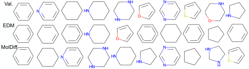
Rings An erroneous generation of bonds will violate the graph topology of the molecules and easily result in biased ring distributions. For instance, adding unnecessary bonds will lead to redundant or unrealistic rings. We thus further extended the analysis of bonds to rings. First, we compare the distributions of counts of rings in each molecule between generated molecules and the validation set. Next, we compared the distributions of counts of -sized rings between generated molecules and validation set using JS divergence and then averaged all JS divergence for . Real molecules usually have plenty of 6-sized rings but much fewer large or small rings and thus we want to check whether the model learned such underlying design principles. Finally, we found out the most frequent ten types of rings in the validation set and generated molecules respectively, and calculated the numbers of frequent rings existing in both the validation set and the generated molecules. As shown in Tab. 2, MolDiff produced better distributions of counts of rings and -sized rings. Regarding the ring types, MolDiff generated much more realistic ones. We also displayed the most frequent ten rings among molecules in the validation set, generated by EDM and by MolDiff in Fig. 3, where it is obvious that most rings generated by EDM were unrealistic as a result of erroneous bonds while those generated by MolDiff were similar with the validation set.
4.3 Analyses of the Noise Schedule and the Guidance
To study the importance of different components, we conducted an ablation study to show the effectiveness of the guidance and the special noise schedule. We compared the complete MolDiff with three variants: (1) the model without the guidance of the bond predictor; (2) the model without using the newly proposed noise schedule, and 3) the model with neither of these two techniques. Tab. 3 demonstrated that both the guidance and new noise schedule could greatly boost the determination of 3D structures. The two strategies also contributed to more realistic counts of bonds. We also found that they had no effect on balancing different bond types. Another observation was that both strategies can benefit the arrangement of the count of rings and different ring types. Therefore, we conclude that the guidance of the bond predictor and the new noise schedule are necessary components to generate molecules with better 3D structures and distributions of bonds and rings. In addition, we found these two strategies did not harm the basic metrics such as generation abilities and drug-likeness as shown in Appendix C.3.
4.4 Model Analysis

Finally, we explored how the noise schedule and the guidance worked. As we mentioned above, the new noise schedule diffused the bond types earlier to avoid the irrational relationship between bonds and atoms during diffusion. We first calculated the ranges of bond lengths of real molecules in the validation set and then counted real bonds whose lengths were out of the range at different steps during the diffusion process. As shown in Fig. 4(a), the noise schedule of MolDiff induced much fewer bonds that were out of range. Actually, these bonds were unnecessary to learn at the current moment, and thus the noise schedule of MolDiff enabled the model to focus on more meaningful data distributions. As for the guidance of the bond predictor, we showed an example demonstrating how it guided the generation of positions in Fig. 4(b)-(d). We perturbed the position of one atom of a molecule in the dataset along the -axis (Fig. 4(b)) and calculated the values and their scaled gradients w.r.t perturbations (Fig. 4(c,d)). We found that as the atom deviated from the ground truth position, the confidence values decreased and the gradients also deviated from zero. Therefore, the gradients of the confidence function assisted to push the atoms to the right positions. In conclusion, both the schedule and guidance facilitate MolDiff to better learn and generate molecules with more accurate 3D structures and more realistic distributions of bonds and rings.
5 Conclusion
In this work, we propose a 3D molecule generation model to simultaneously address the generation of atoms and bonds of molecules. Experimental results demonstrate that the model has greatly improved the generation ability and the quality of the generated molecules. Further work can explore more sophisticated noise schedules and more advanced guidance strategies, and analyze its potential for downstream real tasks.
Acknowledgement
We thank Shitong Luo and Xingchao Liu for the useful discussions. We thank the anonymous reviewers for their insightful reviews. This work is supported by the National Key R&D Program of China No. 2021YFF1201600.
References
- Austin et al. (2021) Austin, J., Johnson, D. D., Ho, J., Tarlow, D., and van den Berg, R. Structured denoising diffusion models in discrete state-spaces. Advances in Neural Information Processing Systems, 34:17981–17993, 2021.
- Axelrod & Gómez-Bombarelli (2022) Axelrod, S. and Gómez-Bombarelli, R. Geom, energy-annotated molecular conformations for property prediction and molecular generation. Scientific Data, 9(1):185, 2022. doi: 10.1038/s41597-022-01288-4. URL https://doi.org/10.1038/s41597-022-01288-4.
- Dhariwal & Nichol (2021) Dhariwal, P. and Nichol, A. Diffusion models beat gans on image synthesis. Advances in Neural Information Processing Systems, 34:8780–8794, 2021.
- Gebauer et al. (2019) Gebauer, N., Gastegger, M., and Schütt, K. Symmetry-adapted generation of 3d point sets for the targeted discovery of molecules. Advances in Neural Information Processing Systems, 32, 2019.
- Gómez-Bombarelli et al. (2018) Gómez-Bombarelli, R., Wei, J. N., Duvenaud, D., Hernández-Lobato, J. M., Sánchez-Lengeling, B., Sheberla, D., Aguilera-Iparraguirre, J., Hirzel, T. D., Adams, R. P., and Aspuru-Guzik, A. Automatic chemical design using a data-driven continuous representation of molecules. ACS central science, 4(2):268–276, 2018.
- Guan et al. (2022) Guan, J., Qian, W. W., Liu, Q., Ma, W.-Y., Ma, J., and Peng, J. Energy-inspired molecular conformation optimization. In International Conference on Learning Representations, 2022.
- Guan et al. (2023) Guan, J., Qian, W. W., Peng, X., Su, Y., Peng, J., and Ma, J. 3d equivariant diffusion for target-aware molecule generation and affinity prediction. In The Eleventh International Conference on Learning Representations, 2023. URL https://openreview.net/forum?id=kJqXEPXMsE0.
- Haefeli et al. (2022) Haefeli, K. K., Martinkus, K., Perraudin, N., and Wattenhofer, R. Diffusion models for graphs benefit from discrete state spaces. arXiv preprint arXiv:2210.01549, 2022.
- Ho et al. (2020) Ho, J., Jain, A., and Abbeel, P. Denoising diffusion probabilistic models. Advances in Neural Information Processing Systems, 33:6840–6851, 2020.
- Hoogeboom et al. (2021) Hoogeboom, E., Nielsen, D., Jaini, P., Forré, P., and Welling, M. Argmax flows and multinomial diffusion: Learning categorical distributions. Advances in Neural Information Processing Systems, 34, 2021.
- Hoogeboom et al. (2022) Hoogeboom, E., Satorras, V. G., Vignac, C., and Welling, M. Equivariant diffusion for molecule generation in 3d. arXiv preprint arXiv:2203.17003, 2022.
- Igashov et al. (2022) Igashov, I., Stärk, H., Vignac, C., Satorras, V. G., Frossard, P., Welling, M., Bronstein, M., and Correia, B. Equivariant 3d-conditional diffusion models for molecular linker design. arXiv preprint arXiv:2210.05274, 2022.
- Jin et al. (2018) Jin, W., Barzilay, R., and Jaakkola, T. Junction tree variational autoencoder for molecular graph generation. In International Conference on Machine Learning, pp. 2323–2332. PMLR, 2018.
- Jin et al. (2020) Jin, W., Barzilay, R., and Jaakkola, T. Composing molecules with multiple property constraints. arXiv preprint arXiv:2002.03244, 2020.
- Jo et al. (2022) Jo, J., Lee, S., and Hwang, S. J. Score-based generative modeling of graphs via the system of stochastic differential equations. arXiv preprint arXiv:2202.02514, 2022.
- Kusner et al. (2017) Kusner, M. J., Paige, B., and Hernández-Lobato, J. M. Grammar variational autoencoder. In International Conference on Machine Learning, pp. 1945–1954. PMLR, 2017.
- Li et al. (2021) Li, Y., Pei, J., and Lai, L. Structure-based de novo drug design using 3d deep generative models. Chemical science, 12(41):13664–13675, 2021.
- Lin et al. (2022) Lin, H., Huang, Y., Liu, M., Li, X., Ji, S., and Li, S. Z. Diffbp: Generative diffusion of 3d molecules for target protein binding. arXiv preprint arXiv:2211.11214, 2022.
- Liu et al. (2022) Liu, M., Luo, Y., Uchino, K., Maruhashi, K., and Ji, S. Generating 3d molecules for target protein binding. In International Conference on Machine Learning, 2022.
- Liu et al. (2018) Liu, Q., Allamanis, M., Brockschmidt, M., and Gaunt, A. Constrained graph variational autoencoders for molecule design. Advances in neural information processing systems, 31, 2018.
- Luo et al. (2021) Luo, S., Guan, J., Ma, J., and Peng, J. A 3d generative model for structure-based drug design. Advances in Neural Information Processing Systems, 34, 2021.
- Luo & Ji (2022) Luo, Y. and Ji, S. An autoregressive flow model for 3d molecular geometry generation from scratch. In International Conference on Learning Representations (ICLR), 2022.
- Malinin & Gales (2018) Malinin, A. and Gales, M. Predictive uncertainty estimation via prior networks. Advances in neural information processing systems, 31, 2018.
- Nichol & Dhariwal (2021) Nichol, A. Q. and Dhariwal, P. Improved denoising diffusion probabilistic models. In International Conference on Machine Learning, pp. 8162–8171. PMLR, 2021.
- Niu et al. (2020) Niu, C., Song, Y., Song, J., Zhao, S., Grover, A., and Ermon, S. Permutation invariant graph generation via score-based generative modeling. In International Conference on Artificial Intelligence and Statistics, pp. 4474–4484. PMLR, 2020.
- O’Boyle et al. (2011) O’Boyle, N. M., Banck, M., James, C. A., Morley, C., Vandermeersch, T., and Hutchison, G. R. Open babel: An open chemical toolbox. Journal of cheminformatics, 3(1):1–14, 2011.
- Peng et al. (2022) Peng, X., Luo, S., Guan, J., Xie, Q., Peng, J., and Ma, J. Pocket2Mol: Efficient molecular sampling based on 3D protein pockets. In Chaudhuri, K., Jegelka, S., Song, L., Szepesvari, C., Niu, G., and Sabato, S. (eds.), Proceedings of the 39th International Conference on Machine Learning, volume 162 of Proceedings of Machine Learning Research, pp. 17644–17655. PMLR, 17–23 Jul 2022. URL https://proceedings.mlr.press/v162/peng22b.html.
- Ragoza et al. (2020) Ragoza, M., Masuda, T., and Koes, D. R. Learning a continuous representation of 3d molecular structures with deep generative models. arXiv preprint arXiv:2010.08687, 2020.
- Ramesh et al. (2022) Ramesh, A., Dhariwal, P., Nichol, A., Chu, C., and Chen, M. Hierarchical text-conditional image generation with clip latents. arXiv preprint arXiv:2204.06125, 2022.
- Roney et al. (2022) Roney, J. P., Maragakis, P., Skopp, P., and Shaw, D. E. Generating realistic 3d molecules with an equivariant conditional likelihood model, 2022. URL https://openreview.net/forum?id=Snqhqz4LdK.
- Satorras et al. (2021a) Satorras, V. G., Hoogeboom, E., Fuchs, F. B., Posner, I., and Welling, M. E (n) equivariant normalizing flows. arXiv preprint arXiv:2105.09016, 2021a.
- Satorras et al. (2021b) Satorras, V. G., Hoogeboom, E., and Welling, M. E (n) equivariant graph neural networks. In International Conference on Machine Learning, pp. 9323–9332. PMLR, 2021b.
- Schneuing et al. (2022) Schneuing, A., Du, Y., Harris, C., Jamasb, A., Igashov, I., Du, W., Blundell, T., Lió, P., Gomes, C., Welling, M., et al. Structure-based drug design with equivariant diffusion models. arXiv preprint arXiv:2210.13695, 2022.
- Segler et al. (2018) Segler, M. H., Kogej, T., Tyrchan, C., and Waller, M. P. Generating focused molecule libraries for drug discovery with recurrent neural networks. ACS central science, 4(1):120–131, 2018.
- Shi et al. (2020) Shi, C., Xu, M., Zhu, Z., Zhang, W., Zhang, M., and Tang, J. Graphaf: a flow-based autoregressive model for molecular graph generation. arXiv preprint arXiv:2001.09382, 2020.
- Song & Ermon (2019) Song, Y. and Ermon, S. Generative modeling by estimating gradients of the data distribution. Advances in Neural Information Processing Systems, 32, 2019.
- Song et al. (2020) Song, Y., Sohl-Dickstein, J., Kingma, D. P., Kumar, A., Ermon, S., and Poole, B. Score-based generative modeling through stochastic differential equations. arXiv preprint arXiv:2011.13456, 2020.
- Vignac et al. (2022) Vignac, C., Krawczuk, I., Siraudin, A., Wang, B., Cevher, V., and Frossard, P. Digress: Discrete denoising diffusion for graph generation. arXiv preprint arXiv:2209.14734, 2022.
- Vignac et al. (2023) Vignac, C., Osman, N., Toni, L., and Frossard, P. Midi: Mixed graph and 3d denoising diffusion for molecule generation. arXiv preprint arXiv:2302.09048, 2023.
- Weininger (1988) Weininger, D. Smiles, a chemical language and information system. 1. introduction to methodology and encoding rules. Journal of chemical information and computer sciences, 28(1):31–36, 1988.
- Wu et al. (2022) Wu, L., Gong, C., Liu, X., Ye, M., and qiang liu. Diffusion-based molecule generation with informative prior bridges. In Oh, A. H., Agarwal, A., Belgrave, D., and Cho, K. (eds.), Advances in Neural Information Processing Systems, 2022. URL https://openreview.net/forum?id=TJUNtiZiTKE.
- Xu et al. (2022) Xu, M., Yu, L., Song, Y., Shi, C., Ermon, S., and Tang, J. Geodiff: A geometric diffusion model for molecular conformation generation. arXiv preprint arXiv:2203.02923, 2022.
- You et al. (2018) You, J., Liu, B., Ying, R., Pande, V., and Leskovec, J. Graph convolutional policy network for goal-directed molecular graph generation. arXiv preprint arXiv:1806.02473, 2018.
- Zhou et al. (2019) Zhou, Z., Kearnes, S., Li, L., Zare, R. N., and Riley, P. Optimization of molecules via deep reinforcement learning. Scientific reports, 9(1):1–10, 2019.
Appendix A More Details about the Model
A.1 Hyper-parameters of the Neural Networks and Training
We set the embedding dimensions of node types and edge types as 256 and 64, respectively and all intermediate hidden dimensions are constant. The time embedding dimensions are 10. The graph neural networks contain six layers. We trained the diffusion network using AdamW optimizer with a learning rate and batch size 256 for iterations. For the weights of the atom loss and bond loss, i.e., and , we set so that the losses of atom types, atom positions, and bond types were almost in the same magnitude. The source codes will be provided at https://github.com/pengxingang/MolDiff.
A.2 Details about the Diffusion Process
A.3 Details about the Model Architectures
Here we detailedly describe the architectures of the neural networks defined in Eq. 3, i.e., , , , and .
The network takes as input the edge feature vector and the edge lengths . It applies RBF kernels to the distance and then combines them with the input feature vector. Finally, it applies a linear layer to process the concatenated feature to the new feature vector .
The network takes as input the vertex feature vectors , the edge feature vector , and the step and outputs the message from vertex to vertex (denoted as ):
| (10) | ||||
where means concatenating along the feature dimension and is the sigmoid activation function.
The network takes as input the vertex feature vectors , the edge feature vector , and the step and outputs the message from the edge (denoted as ):
| (11) | ||||
Finally, the network takes as input the vertex feature vectors , the edge feature vector and step and outputs a scalar :
| (12) | ||||
A.4 Details about the Noise Schedule
The cosine noise schedule is a popular schedule that defines the schedule of using a cosine function and achieves better performance than other schedules (Nichol & Dhariwal 2021). However, the cosine schedule only has one tuneable hyper-parameter and thus it is hard to adapt the shape and the range of the schedule curve of . We define a new schedule scheme that utilizes the sigmoid function and possess three tuneable hyper-parameters to adapt the schedule curve. The schedule is defined as:
| (13) | ||||
The parameters and represent the values of and , respectively, controlling the range of the noise. The parameter influences the slope at medium steps and controls how fast changes at the beginning and the end of the diffusion process. We show how the parameter influences the shapes in Fig. 5.
In our implementation, we chose the parameters for atom types and atom positions for the whole diffusion process . For the bond type, we used during diffusion steps in the first stage and during steps in the second stage. The curves of MolDiff are shown in Fig. 6
A.5 Details about the Bond Predictor
The bond predictor has almost the same architecture as the main diffusion neural networks except for two differences. First, the bond predictor does not need the position updates. Second, the initial input edge features do not contain the bond types of the edge. Instead, we provide the atom types of the two ends of the edges as the initial edge features.
The bond predictor was trained using the same dataset as the diffusion network. The training uses the same noise schedules of the atom positions and atom types. At step , the bond predictor takes as input the noised atom positions , atom types and step and predicts the bond types at step 0, i.e., . The loss function is the cross-entropy between the predicted bond types and the ground truth. We trained the bond predictor using AdamW optimizer with a learning rate and batch size 256 for iterations.
Appendix B Preprocessing of the Geom-Drug Dataset
We downloaded the GEOM-Drug from the database website (Axelrod & Gómez-Bombarelli 2022). We filtered the molecules through the following criterion: (1) can be parsed by the RDKit package; (2) not broken; (3) the number of heavy atoms within ; (4) not contain the elements other than H, C, N, O, F, P, S, and Cl; (5) not contain chemical bonds other than single, double, triple and aromatic bonds. After filtering, we removed the hydrogen atoms and constructed the training, validation, and testing datasets with 231523, 28941, and 28940 molecules, respectively.
Appendix C More Details and Results about the Experiments
C.1 Details about the Experiment Settings and Baselines
In all experiments, we kept generating molecules until there were 1000 valid and complete molecules and then calculated metrics according to their definitions. We repeated this for three times and reported the average values in the main text and standard deviations in the Appendix C.4.
We re-trained the baseline EDM using our splittings of the GEOM-Dataset dataset. For the variants of MolDiff that did not incorporate the bond types during diffusion, we removed the edge updates in Eq. 3, and the initial edge embedding did not contain the information of bond type. Three different bond post-predicting strategies were considered for three different models: First, a lookup table that was the same as the one used by EDM was utilized to match the bond lengths with the atom distances. Second, the NN-based bond predictor that was originally used for the guidance was applied to predict the bond types after diffusion. Third, the chemical toolkit Open Babel was applied to add the chemical bonds. For the variants of MolDiff that used continuous diffusion for both atom and bond types, they regarded the one-hot embedding of the types as continuous values in the latent spaces and added Gaussian noise. The scaling for continuous diffusion was to divide the one-hot embedding of the atom and bond types by scalars before diffusion, which was proposed by the authors of EDM. We set the scaling for the atom types, atom positions, and bond types as 1, 4, and 8, respectively. For the variant with bond length loss, we further added an MSE loss to minimize the difference between the real bond lengths with the predicted ones for pairs that were not none-type, which is a simple method to attempt to generate more accurate bond lengths. Note all these variants did not use the newly proposed noise schedule and the guidance.
C.2 Details about the Metrics
For the metric of drug-likeness, we borrowed the evaluation code from Pocket2Mol (Peng et al. 2022). For the analyses of bond lengths, the SMARTS (SMILES arbitrary target specification) of considered bond types were: c:c, [#6]-[#6], [#6]-[#7], [#6]-O, c:n, [#6]=O, [#6]-S, O=S, c:o, c:s, [#6]-F, n:n, [#6]-Cl, [#6]=[#6], [#7]-S, [#6]=[#7], [#7]-[#7], [#7]-O, [#6]=S, and [#7]=O. For the analyses of bond angles, the SMARTS of considered bond pairs were: c:c:c, [#6]-[#6]-[#6], [#6]-[#7]-[#6], [#7]-[#6]-[#6], c:c-[#6], [#6]-O-[#6], O=[#6]-[#6], [#7]-c:c, n:c:c, c:c-O, c:n:c, [#6]-[#6]-O, and O=[#6]-[#7]. The SMARTS of considered bond triplets were: c:c:c:c, [#6]-[#6]-[#6]-[#6], [#6]-[#7]-[#6]-[#6], [#6]-c:c:c, [#7]-[#6]-[#6]-[#6], [#7]-c:c:c, O-c:c:c, [#6]-[#7]-c:c, [#7]-[#6]-c:c, n:c:c:c, [#6]-[#7]-[#6]=O, [#6]-[#6]-c:c, c:c-[#7]-[#6], c:n:c:c, and [#6]-O-c:c.
C.3 Details and More Results of the Ablation Study
For the variant without guidance, we removed the guidance term in Eq. 6 during generation. For the variant without the new noise schedule, the schedule of bond type was the same as that of the atoms. In Tab. 4, we reported the generation abilities and the drug-likeness properties of the ablation study, which indicated that the our proposed noise schedule and the guidance of the bond predictor did not damage these basic properties.
| Validity | Connec-tivity | Succ. rate | Novelty | Diversity | Unique- ness | Sim. Val. | QED | SA | Lipinski | |
| MolDiff | 0.997 | 0.996 | 0.993 | 0.972 | 0.769 | 0.986 | 0.634 | 0.668 | 0.874 | 4.986 |
| No Gui. | 0.992 | 0.964 | 0.956 | 0.983 | 0.763 | 0.995 | 0.603 | 0.680 | 0.825 | 4.985 |
| No Sche. | 1.000 | 0.993 | 0.993 | 0.985 | 0.766 | 0.998 | 0.639 | 0.692 | 0.862 | 4.951 |
| Neither | 0.999 | 0.971 | 0.970 | 0.990 | 0.764 | 0.999 | 0.628 | 0.710 | 0.822 | 4.941 |
C.4 Standard Deviations of the Values in the Main Text.
To facilitate the comparison of the metric values of different models, here we provided the standard deviations of those values in the tables of the Sec. 4 (i.e., Tab. 1, 2, and 3) in Tab. 5, 6, and 7.
| Validity | Connectivity | Novelty | Diversity | |
| EDM | 0.0002 | 0.0068 | 0.0000 | 0.0033 |
| MolDiff | 0.0012 | 0.0014 | 0.0024 | 0.0004 |
| Predict bond(Lookup table) | 0.0035 | 0.0075 | 0.0000 | 0.0045 |
| Predict bond(NN Predictor) | 0.0016 | 0.0027 | 0.0065 | 0.0025 |
| Predict bond(Openbabel) | 0.0023 | 0.0043 | 0.0037 | 0.0024 |
| Conti. Diffusion | 0.0116 | 0.0142 | 0.0004 | 0.0010 |
| Conti. Diffusion(scaling) | 0.0014 | 0.0027 | 0.0005 | 0.0039 |
| Add bond length loss | 0.0008 | 0.0030 | 0.0021 | 0.0028 |
| Group | Metrics | EDM | MolDiff |
| Drug-likeness | QED | 0.0059 | 0.0050 |
| SA | 0.0038 | 0.0021 | |
| Lipinski | 0.0076 | 0.0029 | |
| 3D structures | RMSD | 0.0121 | 0.0156 |
| JS. bond lengths | 0.0033 | 0.0079 | |
| JS. bond angels | 0.0120 | 0.0070 | |
| JS. dihedral angles | 0.0031 | 0.0027 | |
| Bonds | JS. #bonds per atoms | 0.0187 | 0.0051 |
| JS. basic bond types | 0.0016 | 0.0027 | |
| JS. freq. bond types | 0.0012 | 0.0019 | |
| JS. freq. bond angles | 0.0028 | 0.0025 | |
| JS. freq. bond triplets | 0.0043 | 0.0025 | |
| Rings | JS. #rings | 0.0179 | 0.0040 |
| JS. #n-sized rings | 0.0034 | 0.0020 | |
| #Intersecting rings | 0.4714 | 0.0000 |
| Metrics | No Gui. | No Sche. | Neither | Metrics | No Gui. | No Sche. | Neither |
| Validity | 0.0009 | 0.0005 | 0.0000 | JS. bond lengths | 0.0152 | 0.0066 | 0.0133 |
| Connectivity | 0.0025 | 0.0008 | 0.0049 | JS. bond angels | 0.0052 | 0.0060 | 0.0057 |
| Novelty | 0.0012 | 0.0038 | 0.0005 | JS. dihedral angles | 0.0034 | 0.0041 | 0.0043 |
| Diversity | 0.0012 | 0.0023 | 0.0014 | JS. #bonds per atoms | 0.0008 | 0.0051 | 0.0108 |
| Uniqueness | 0.0016 | 0.0017 | 0.0000 | JS. basic bond types | 0.0026 | 0.0019 | 0.0017 |
| Sim. Val | 0.0023 | 0.0018 | 0.0012 | JS. freq. bond types | 0.0023 | 0.0038 | 0.0024 |
| QED | 0.0024 | 0.0016 | 0.0052 | JS. freq. bond angles | 0.0026 | 0.0031 | 0.0032 |
| SA | 0.0040 | 0.0004 | 0.0030 | JS. freq. bond triplets | 0.0041 | 0.0029 | 0.0033 |
| Lipinski | 0.0016 | 0.0028 | 0.0048 | JS. #rings | 0.0067 | 0.0056 | 0.0032 |
| RMSD | 0.0174 | 0.0056 | 0.0093 | JS. #n-sized rings | 0.0033 | 0.0017 | 0.0048 |
| #Intersecting rings | 0.4714 | 0.0000 | 0.0000 |
C.5 More Examples of Generated Molecules
We showed the 3D conformations and the 2D graphs of several molecules generated by MolDiff in Fig. 7 and Fig. 8.


Appendix D Additional evaluations on more datasets
In the main text, we assessed models on the molecules only containing major elements in the GEOM-Drug dataset and removed hydrogen atoms when training and evaluation. Here, we conducted additional experiments on three more datasets: 1) molecules in the GEOM-Drug dataset containing major elements but with hydrogens reserved; 2) molecules in the GEOM-Drug dataset containing all elements; 3) a different dataset QM9 dataset. Note in these experiments, the sampling of MolDiff did not use the guidance of bond predictor.
D.1 Evaluation on Molecules with Hydrogens Reserved
The reason that we removed the hydrogens was from a practical perspective because hydrogens can be easily speculated from the heavy atoms and were often omitted in molecule representations in practical scenarios. However, the inclusion of hydrogens resulted in bigger graphs for a more rigid benchmark, which can help us understand the behaviors of models. Therefore, we have added an experiment to incorporate all hydrogen atoms.
As shown in Tab. 8, compared to the performance without hydrogens (the result of one repeat in our original dataset), MolDiff performed worse in the dataset with hydrogens, especially the connectivity and thus the success rate. This discrepancy was caused by the fact that the inclusion of hydrogens made the average number of atoms per molecule raised from around 24 to around 45, resulting in much more complicated molecular graphs. But the success rate of MolDiff with hydrogens (0.739) was still higher than EDM even without hydrogens (0.371 in Tab. 1) and the qualities of the generated molecules were not obviously influenced by the inclusion of hydrogens.
| Dataset | With hydrogen | Without hydrogen |
| Validity | 0.993 | 0.957 |
| Connectivity | 0.961 | 0.772 |
| Succ. Rate | 0.954 | 0.739 |
| Novelty | 0.983 | 1.000 |
| Uniquness | 0.997 | 1.000 |
| Diversity | 0.761 | 0.427 |
| Sim. Val. | 0.603 | 0.695 |
| QED | 0.677 | 0.688 |
| SA | 0.821 | 0.806 |
| Lipinski | 4.983 | 4.868 |
| RMSD. | 1.005 | 1.032 |
| JS. bond lengths | 0.374 | 0.414 |
| JS. bond angles | 0.168 | 0.182 |
| JS. dihedral angles | 0.205 | 0.244 |
D.2 Comparison between MolDiff and EDM on Molecules with All Elements
Previously, we excluded some minor element types (B, Br, I, Si, Bi) from the GEOM-Drug dataset during data processing because they are not commonly used in drug design compared to other elements (C, N, O, F, P, S, Cl). Additionally, the generation of molecules containing these minor elements may bring more difficulties in subsequent biochemical experiments. Moreover, these minor elements accounted for less than 0.2% of the GEOM-drug dataset, making it difficult for the models to properly learn their features. For instance, there were only 12 Si atoms in the entire GEOM-Drug dataset, and it was challenging for a model to learn how to generate Si atoms from these samples.
However, it is interesting to see how the model performs on the complete dataset. Therefore, we added an experiment to train our model on the complete GEOM-Drug dataset (i.e., all elements were used and hydrogens were not removed). The comparison of MolDiff and EDM on this complete dataset was shown in Tab. 9.
The performances of both MolDiff and EDM decreased compared to those in the original filtered dataset (i.e., the dataset used in the main text). But MolDiff still had high generation ability with a success rate of 0.860. However, the EDM model had a much lower success rate of 0.014, indicating that 100 samples resulted in about one valid and complete molecule, which was of little use for practical applications. Therefore, EDM cannot work on this complete GEOM-Drug dataset while MolDiff still worked well. Regarding the qualities of generated molecules, the superiority of MolDiff over EDM in the complete was the same as that in the filtered dataset. Therefore, working on the complete dataset, MolDiff performed slightly worse than in the filtered dataset but still much better than EDM.
| Model | MolDiff | EDM |
| Validity | 0.947 | 0.029 |
| Connectivity | 0.908 | 0.484 |
| Succ. Rate | 0.860 | 0.014 |
| Novelty | 1.000 | 1.000 |
| Uniquness | 1.000 | 1.000 |
| Diversity | 0.422 | 0.455 |
| Sim. Val. | 0.696 | 0.668 |
| QED | 0.700 | 0.536 |
| SA | 0.805 | 0.624 |
| Lipinski | 4.874 | 4.839 |
| RMSD. | 0.963 | 1.103 |
| JS. bond lengths | 0.472 | 0.439 |
| JS. bond angles | 0.178 | 0.435 |
| JS. dihedral angles | 0.228 | 0.605 |
D.3 Comparison on QM9 dataset
QM9 dataset was widely adopted to benchmark previous 3D molecule generation models. We did not adopt it as our main dataset because the molecules are simpler and less drug-like than those in the GEOM-Drug dataset. Here we add a comparison on the QM9 dataset with more baselines, including EDM(Hoogeboom et al. 2022), EN-flow(Satorras et al. 2021a), G-Schnet(Gebauer et al. 2019), and G-SphereNet(Luo & Ji 2022). We followed the setup of EDM to split the QM9 dataset with train/validation/test size as 100k/18k/13k.
We compared the generation abilities and the accuracy of 3D geometries of these methods, as shown in Tab. 10. MolDiff showed the best generation ability (with the highest validity, connectivity, and success rate), indicating that MolDiff generated more valid and complete molecules than the others. Although EDM showed better performance in the QM9 dataset than it in the GEOM-Drug dataset, it still showed a relatively weaker generation ability than MolDiff. Regarding the novelty, diversity, uniqueness, and similarity with the validation set, these methods achieved similar performance. For 3D geometries, MolDiff achieved the best performance in terms of RMSD and the JS. divergence of dihedral angles and was second-best for the JS. divergence of bond lengths and bond angles, with the differences among methods being less significant. Overall, MolDiff maintained its superior generation abilities and accuracy of 3D geometries on the QM9 dataset, although the margin over other methods was smaller due to the relative simplicity of molecules in QM9 compared to those in the GEOM-Drug dataset.
| MolDiff | EDM | EN-flow | G-SchNet | G-SphereNet | |
| Validity | 0.970 | 0.925 | 0.407 | 0.876 | 0.161 |
| Connectivity | 0.998 | 0.992 | 0.604 | 0.997 | 0.998 |
| Succ. rate | 0.968 | 0.918 | 0.246 | 0.873 | 0.161 |
| Novelty | 1.000 | 1.000 | 1.000 | 1.000 | 1.000 |
| Diversity | 0.894 | 0.893 | 0.892 | 0.875 | 0.658 |
| Uniqueness | 0.991 | 0.999 | 0.999 | 0.995 | 0.225 |
| Sim. Val. | 0.705 | 0.602 | 0.490 | 0.628 | 0.732 |
| RMSD | 0.193 | 0.249 | 0.587 | 0.278 | 0.199 |
| JS. bond lengths | 0.340 | 0.231 | 0.513 | 0.342 | 0.367 |
| JS. bond angles | 0.158 | 0.105 | 0.367 | 0.193 | 0.334 |
| JS. dihedral angles | 0.368 | 0.383 | 0.713 | 0.492 | 0.721 |