Sequential Experimental Design for Spectral Measurement:
Active Learning Using a Parametric Model

As shown in the Fig. 1, the measurement points have different levels of importance in the spectral measurement; however, the shape of the spectrum is unknown before the experiment is performed. Therefore, it is better to focus on the important measurement points by selecting the next measurement points from the currently obtained data. Here, we consider a sequential experimental design that considers two spectral measurement constraints. The first constraint is that the resolution of the horizontal axis is fixed. This limits the measurement points to a finite set $\mathcal{X}$. Thus, we first perform short measurements for all points on $\mathcal{X}$ and subsequently actively select points that need to be measured repeatedly. The second constraint is that, due to the nature of the measurement instrument, the energy of the irradiated photons can only increase, and the number of times where the minimum energy increases to the maximum energy should be decreased. Therefore, from the given data, we reduced the number of scans by selecting multiple $x\in\mathcal{X}$ as the next measurement points.

The formulation of the sequential experimental design is as follows. Suppose that $D=\{(x_{1},y_{1}),...,(x_{N},y_{N})\}$ is given as the initial data. Given data $D$, we choose $\{x_{next,1},...,x_{next,n}\}$ from a finite set $\mathcal{X}$ as the next measurement points and observe $\{y_{next,1},...,y_{next,n}\}$. Thereafter, we update data $D$ by adding $\{(x_{next,1},y_{next,1}),...,(x_{next,n},y_{next,n})\}$. We repeat this update $k$ times. For a measurement point $x_{i}$, we define the total measurement time per measurement time as $t_{i}=\#\{j|x_{j}=x_{i}\}\times(\textup{time per measurement})$ and the observed values per total measurement time as $\bar{y}_{i}=\frac{\sum_{x_{j}=x_{i}}y_{j}}{t_{i}}$. The more measurement point $x_{i}$ is measured repeatedly, the larger the $t_{i}$ value and the better the signal-to-noise ratio of $\bar{y}_{i}$. Therefore, we must consider an algorithm that measures the important measurement points intensively. The flow of the sequential experimental design is shown in Fig. 2. As shown in Fig. 2, in the sequential experimental design, the signal-to-noise ratio is poor at all points at first. However, as the experiment progresses, the signal-to-noise ratio near the peaks improves due to focused measurements.

In this section, we describe a method to realize active learning by Bayesian inference using parametric models and to select the next measurement point. First, we consider the parametric model $(M)$, in which the observed value $(y)$ for a measurement point $(x)$ is generated independently with a probability distribution:

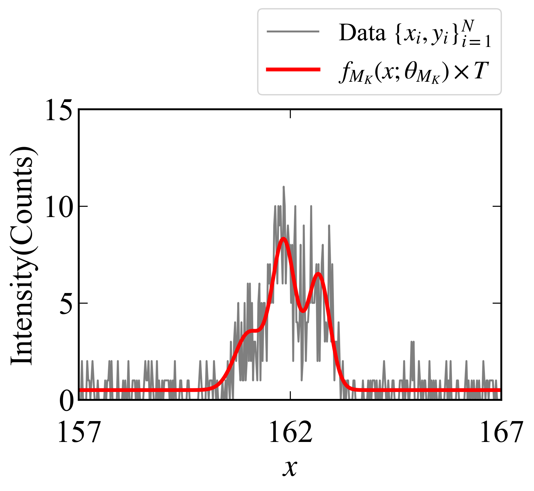
where $\theta_{M}$ is the parameter of $M$, and $f_{M}(x;\theta_{M})$ is the function used for modeling. For example, if we define the sum of three Gaussian functions as the modeling function and the Poisson distribution as the probability distribution, we obtain Fig. 3. This assumes that the values of the modeling function with noise are observed.

From the independence of probability distributions, the probability that data $D=\{x_{i},y_{i}\}_{i=1}^{L}$ is given, assuming that a certain model $M$ and its parameters $(\theta_{M})$ can be formulated as follows:

where $\{x_{i}\}_{i=1}^{n}$ can be chosen by the sequential experimental design. Otherwise, $p(D|\theta_{M})=0$.

From this probabilistic model, we consider estimating the parameters from the data. If $p(\theta_{M}|M)$ is the prior distribution of the model parameters, then the joint probability distribution, $p(D,\theta_{M}|M)$, is as follows:

From Bayes’ theorem, the posterior distribution of parameter $\theta_{M}$, given data $D$ and model $M$, is given by

This posterior distribution can be employed to estimate these parameters. Moreover, we consider selecting the most plausible model from model candidates, such as the selection of the number of peaks in the example shown in Fig. 3. Let $\mathcal{M}$ be the set of model candidates and $p(M)$ be the prior distribution of the model. Thus, the joint probability $(p(D,\theta_{M},M))$ is given by

From Bayes’ theorem, the posterior distribution of model $M$, given data $D$, is as follows:

This posterior distribution can be employed to select a plausible model. For various cases of $p(y|f_{M}(x;\theta_{M}))$, the numerical sampling of $p(\theta_{M}|D,M)$ and the numerical computation of $p(M|D)$ can be realized by the exchange Monte Carlo method Nagata et al. 2012; Nagata et al. 2019; Mototake et al. 2019; Hukushima and Nemoto 1996.

Using the posterior distribution $(p(M|D),p(\theta_{M}|D,M))$, we consider the estimation uncertainty at the measurement points of each model to select the next measurement points. We assume that the model candidate set $(\mathcal{M})$, a prior distribution of models $(p(M))$, and a prior distribution of parameters $(p(\theta_{M}|M))$ are given. Let $D=\{x_{i},y_{i}\}_{i=1}^{L}$ be the data currently available. We define $\widehat{M}=\max_{M\in\mathcal{M}}p(M|D)$ as the best predicted model and $M^{\circ}=\max_{M\neq\widehat{M}}p(M|D)$ as the second-best predicted model. Furthermore, we define the best model map estimator of parameter $\grave{\theta}=\max_{\theta_{\widehat{M}}}p(\theta_{\widehat{M}}|D,\widehat{M})$ and the estimator of the modeling function, $\grave{f}(x)=f_{\widehat{M}}(x;\grave{\theta})$. Here, we formulate the estimated uncertainties, i.e., $G(x;\widehat{M})$ and $G(x;M^{\circ})$, for models $\widehat{M}$ and $M^{\circ}$, respectively, at the measurement point $x$, as follows:

These formulations calculate the distance between the probability distribution $(p(y|\grave{f}(x)))$ and $(p(y|f(x;\theta_{\widehat{M}})),p(y|f(x;\theta_{M^{\circ}})))$, obtained from the posterior distribution $(p(\theta_{M}|M,D))$ of each model. These integrations can be computed by the exchange Monte Carlo sampling of $p(\theta_{M}|M,D)$.

Using this estimation uncertainty, we describe a method for selecting the next measurement point. We choose $\{x_{next,1},...,x_{next,\frac{n}{2}}\}$ and $\{x_{next,\frac{n}{2}+1},...,x_{next,n}\}$ from $\mathcal{X}$, where $G(x;\widehat{M})$ and $G(x;M^{\circ})$ are large, respectively. The selection of points using $G(x;\widehat{M})$ corresponds to focusing on important points for the parameter estimation of the best predicted model, and selecting points using $G(x;M^{\circ})$ corresponds to focusing on the difference between the best predicted model and the second-best predicted model.

In Eq. 7 and 8, $\textup{KL}(x,y)$ is the Kullback – Leibler divergence of $x$ and $y$. For photon counting measurements, such as XPS, the probability distribution of the observed data $(p(y|f_{M}(x;\theta_{M})))$ is considered to be

with T representing the measurement time. Thus, the Kullback–Leibler divergence is expressed as follows:

Thus, the value of $T$ does not change the selection result in this method.

Although there are other possible selection methods, in this study, we focused on this method and evaluated its effectiveness through numerical experiments. Furthermore, this method can also be applied in the problem setting where the model is fixed by setting $\widehat{M}=M^{\circ}$.

We consider a model in which the expected value of the XPS observation per unit time is represented by a linear sum of multiple peaks and backgrounds. Let $M_{K}$ be a model with $K$ peaks, the parameter set $(\theta_{M_{K}})$ be $\theta_{M_{K}}=\{\{a_{k},\mu_{k},\sigma_{k}\}_{k=1}^{K},B\}$, and the modeling function $(f_{M_{K}}(x;\theta_{K}))$ be $f_{M_{K}}(x;\theta_{K})=\sum_{k=1}^{K}a_{k}\exp\left(-\frac{(x-\mu_{k})^{2}}{\sigma_{k}^{2}}\right)+B$ (where $a_{k},\mu_{k},\sigma_{k}$, and $B$ correspond to the peak intensity, peak position, peak width, and background intensity, respectively). Since the measurement is performed by photon counting in XPS, the probability distribution of the number of observed photons $(p(y|f_{M}(x;\theta_{M})))$ is considered to be $\textup{Poisson}(y;f_{M}(x;\theta_{M})\times T)$ with measurement time $T$. The posterior distributions, $p(M_{K}|D),p(\theta_{K}|D,M_{K})$, for data $D=\{(x_{1},y_{1}),...,(x_{N},y_{N})\}$ can be obtained by the exchange Monte Carlo method Nagata et al. 2019. In this problem setting, the goal is to select the number of peaks and estimate the parameters of the peak positions with high accuracy from experiments with a short total measurement time.

In Sect. III.2, the set of candidate models must be given in advance; however, in the Bayesian spectral deconvolution, the number of peaks $(K)$ can take any integer. Therefore, we consider changing the candidate model set sequentially.

We define the initial model set as $\mathcal{M}=\{M_{1},M_{2}\}$. At each step, let $\widehat{K}$ be the number of peaks of the best predicted model ($\widehat{M}$ ($\widehat{M}=M_{\widehat{K}}$)), and we use the following model set in the next estimation:

The specific algorithm is shown in Algorithm 1.

Let the true model be the model $M_{3}$ with $K=3$ peaks, and the true values of the parameters $(\theta_{M_{3}}^{*}=\{\{a_{k}^{*},\mu_{k}^{*},\sigma_{k}^{*}\}_{k=1}^{3},B^{*}\})$ be as follows:

This true value is the same as that reported by Nagata et al. Nagata et al. 2019, which is set so that the number of peaks is somewhat difficult to estimate. The modeling function $(f_{M_{3}}(x;\theta_{M_{3}}^{*}))$ is shown in Fig. 3. In this situation, let $\eta_{a}=2.0,\lambda_{a}=1.0,$ $\nu_{0}=157.0,\xi_{0}=167.0,\eta_{\sigma}=10.0,\lambda_{\sigma}=2.5,$ $\nu_{B}=0.1,\xi_{B}=0.01$, and we set the prior distributions of $\{a_{k},\mu_{k},\sigma_{k}\}_{k=1}^{K},B$ be set as follows:

where $\Gamma(\eta_{a})$ is the gamma function, $U(\nu_{0},\nu_{1})$ is the uniform distribution on $[\nu_{0},\nu_{1}]$, and $N(B;\nu_{B},{\xi_{B}}^{2})$ is the Gaussian distribution of mean $\nu_{B}$ and variance ${\xi_{B}}^{2}$.

Let the prior distribution of the model set be $\varphi(M_{k})=\frac{1}{|\mathcal{M}|}$, the time for one measurement in the sequential experiment $T$ be $T=1$, the vertical resolution of the experiment be $0.025\ \textup{(eV)}$, the number of data $N$ be $N=400$, and the candidate set of measurement points $\mathcal{X}$ be $\mathcal{X}=\{157+0.025(i-1)\ \textup{(eV)}\}_{i=1}^{400}$. First, we measure all points on $\mathcal{X}$ with a measurement time $T=1$. Thereafter, we repeat the experiment $k=160$ times by sequentially selecting $n=10$ points to be measured next so that the total measurement time $T_{sum}=N\times T+n\times k\times T=2000$. To evaluate the effectiveness of our method, we compare the result with another method in which the total measurement time $T_{sum}=2000$ with $T=5$ at all measurement points and one in which the total measurement time $T_{sum}=6000$ with $T=15$ at all measurement points. We denote these experiments in which the same measurement is conducted at all points as static experiments.

The data and the fitting by the map estimator ($\grave{\theta}_{M_{3}}=\{\{\grave{a}_{k},\grave{\mu}_{k},\grave{\sigma}_{k}\}_{k=1}^{K},\grave{B}\}=\underset{\theta}{\text{argmax}}p(\theta|D,M_{3}))$ are shown in Fig. 4 (The parameter indices are set so that $\mu_{1}<\mu_{2}<\mu_{3}$).

This figure shows that the sequential experimental design focuses on the measurement points near the peaks that are considered to be important in the spectral deconvolution and improve the signal-to-noise ratio near the peaks.

In addition, we estimate the peak position parameters $(\mu_{1},\mu_{2},\mu_{3})$ assuming that the true model $K=3$ (The parameter indices are set so that $\mu_{1}<\mu_{2}<\mu_{3}$). The results of the parameter estimation are shown in Fig. 5.

This figure shows that the width of the posterior distribution is shorter than that for a static experiment with $T_{sum}=2000$, and is similar to that for a static experiment with $T_{sum}=6000$. This result indicates that the time required for the experiment has been reduced to one-third of the original.

Furthermore, we repeat the above trial 10 times independently to confirm the statistical properties. We define the indices to evaluate the width of the peak position parameter estimation as follows:

where

These indices represent the deviations between the 95% confidence intervals of the parameter estimation and the true parameters $\{\mu_{1}^{*},\mu_{2}^{*},\mu_{3}^{*}\}$. The boxplots of $W_{\mu_{1}},W_{\mu_{2}}$, and $W_{\mu_{3}}$ for the 10 trials are shown in Fig. 6.

This figure shows that the estimations afforded by our method are more accurate than those by the static experiment with $T_{sum}=2000$ and are as accurate as those afforded by the static experiment with $T_{sum}=6000$.

Moreover, we calculated the posterior distribution $(P(M_{2}|D),P(M_{3}|D),P(M_{4}|D))$ for the 10 independent trials, with $\mathcal{M}=\{M_{2},M_{3},M_{4}\}$. The bar graphs of $P(M_{2}|D),P(M_{3}|D),P(M_{4}|D)$ are shown in Fig. 7.

This figure shows that the model selection accuracy of our method is higher than that of the static experiment with $T_{sum}=2000$ and is similar to that of the static experiment with $T_{sum}=6000$. These results also indicate that the time required for the experiment has been reduced to one-third of the original.

We consider selecting a better generative model, which is defined by the effective Hamiltonian, using the simplified 4f-electron-derived 3d core-level XPS spectra data of rare-earth insulating compounds. Let $\epsilon_{L},\epsilon_{f}^{0}$ and $\epsilon_{c}$ be the energies of the conducting electrons of 4f rare-earth metals (5d, 6s electrons), the 4f electron, and the core electron, respectively. We set the index $\nu$ ($\nu=1,...,N_{f},N_{f}=14$) as the quantum number of the spin and f orbital. Moreover, let $V,U_{ff}$ and $-U_{fc}$ be the energies of the hybridization interaction between the 4f electrons and the conduction electrons, the Coulomb interaction between the 4f electrons, and the core-hole Coulomb potential for the 4f electrons, respectively. We define $\Delta=\epsilon_{f}^{0}-\epsilon_{L}$. Let $M_{2}$ be a model using a two-state Hamiltonian $(H_{2})$ and $M_{3}$ be a model using a three-state Hamiltonian $(H_{3})$, and let $\mathcal{M}=\{M_{2},M_{3}\}$ be the set of candidate models.

The two-state Hamiltonian $(H_{2})$ is the effective Hamiltonian for the XPS spectrum of $\textup{La}_{2}\textup{O}_{3}$ and was proposed by Kotani and Toyozawa Kotani and Toyozawa 1974. The Hamiltonian is given by

where $\ket{G}$ is the eigenstate of the minimum energy $(E_{G})$ in the initial state and $\ket{F_{j}}(j=0,1)$ is the eigenstate of the two energy levels $(E_{j}(j=0,1))$ in the final state. To compare the two models, we introduce the energy shift parameter $(b)$. Here, we set the parameter $\theta_{M_{2}}=\{\Delta,V,\Gamma,U_{fc},b\}$ and the modeling function as

$H_{3}$ is the effective Hamiltonian for the XPS spectrum of $\textup{Ce}\textup{O}_{2}$ and was proposed by Kotani et al. Kotani et al. 1985. The Hamiltonian is given by

where $\ket{G}$ is the eigenstate of the minimum energy $(E_{G})$ in the initial state, and $\ket{F_{j}}(j=0,1,2)$ is the eigenstate of the three energy levels $(E_{j}(j=0,1,2))$ in the final state. As in the case of $H_{2}$, we introduce the energy shift parameter $(b)$. Here, we set the parameter $\theta_{M_{3}}=\{\Delta,V,\Gamma,U_{fc},U_{ff},b\}$ and the modeling function as follows:

As in Sect. III.1, the probability distribution of the number of observed photons $(p(y|f_{M}(x;\theta_{M})))$ is considered to be $\textup{Poisson}(y;f_{M}(x;\theta_{M})\times T)$, with measurement time $T$. The posterior probability distributions $(p(M_{K}|D),p(\theta_{K}|D,M_{K}))$ for data $D=\{(x_{1},y_{1}),...,(x_{N},y_{N})\}$ can be calculated by the exchange Monte Carlo method Mototake et al. 2019. In this problem setting, our goal is to select better models from $M_{2},M_{3}$ and to estimate the parameters of $\Delta,U_{fc}$ with high accuracy from experiments with a short total measurement time.

Unlike the case in Sect. III.2, the model set $(\mathcal{M}=\{M_{2},M_{3}\})$ is fixed. The specific algorithm is shown in Algorithm 2.

Let the true model be the model $M_{3}$ with $H_{3}$ and the true values of its parameters be as follows:

This true parameter is derived from Mototake et al. Mototake et al. 2019. Although this parameter is different from the real parameter of ${}\mathrm{CeO}{\vphantom{\mathrm{X}}}_{\vphantom{\mathrm{2}}\smash[t]{\mathrm{2}}}^{\vphantom{\smash[t]{\mathrm{2}}}\hphantom{\mathrm{2}}\mathrm{}}$, we set this parameter to complicate the model selection. The modeling function with the true parameter $(\theta_{M_{3}}^{*}=\{\Delta^{*},V^{*},\Gamma^{*},U_{fc}^{*},U_{ff}^{*},b^{*}\})$ is shown in Fig. 8. The peak around $x=5$ is small, indicating that the model selection from model $M_{2}$ that generates two peaks and model $M_{3}$ that generates three peaks is difficult.

In this situation, we set the prior distribution of the parameters as follows:

Let the prior distribution of the model set be $\varphi(M_{2})=\varphi(M_{3})=\frac{1}{2}$, the time for one measurement in the sequential experiment $T$ be $T=6$, the vertical resolution of the experiment be $0.125(eV)$, the number of data $N$ be $N=400$, and the candidate set of measurement points $\mathcal{X}$ be $\mathcal{X}=\{-30+0.125(i-1)\}_{i=1}^{400}$. First, we measure all points on $\mathcal{X}$ with a measurement time of $T=6$. Thereafter, we repeat the experiment $k=160$ times by sequentially selecting $n=10$ points to be measured next so that the total measurement time is $T_{sum}=N\times T+n\times k\times T=12,000$. To evaluate the effectiveness of our method, we compare the result with that of a static experimental design in which the total measurement time is $T_{sum}=12,000$, with $T=30$ at all measurement points and that of an experiment in which the total measurement is $T_{sum}=36,000$, with $T=90$ at all measurement points.

The data and the fitting by the map estimator $(\grave{\theta}_{M_{3}}=\underset{\theta}{\text{argmax}}p(\theta|D,M_{3}))$ are shown in Fig. 9. It can be observed that the area near the peaks, particularly near the small peak around $x=5$, is measured intensively.

In addition, we estimate the parameter of $\Delta,U_{fc}$, assuming that the true model is $M_{3}$. The results of the parameter estimation are shown in Fig. 10.

Furthermore, we repeat the above trial 10 times independently to confirm the statistical property, similar to the case in Sect. III. We define indices to evaluate the width of the parameter estimation, as follows:

where

These indices represent the deviations between the 95% confidence intervals of the parameter estimation and the true parameters $(\Delta^{*},U_{fc}^{*})$. The boxplots of $W_{\Delta},W_{U_{fc}}$ for the 10 trials are shown in Fig. 11. The figure shows that the estimations by our method are more accurate than those by the static experiment with $T_{sum}=12,000$ and are as accurate as those by the static experiment with $T_{sum}=36,000$.

Moreover, we calculate the posterior distribution $(P(M_{2}|D),P(M_{3}|D))$ for the 10 independent trials with $\mathcal{M}=\{M_{2},M_{3}\}$. The bar graphs of $P(M_{2}|D),P(M_{3}|D)$ are shown in Fig. 12. This figure shows that the model selection accuracy by our method is higher than that by the static experiment with $T_{sum}=12,000$ and is similar to that by the static experiment with $T_{sum}=36,000$. These results indicate that the time required for the experiment has been reduced to one-third of the original.

References

- Tolstoy et al. (2003) V. P. Tolstoy, I. Chernyshova, and V. A. Skryshevsky, Handbook of Infrared Spectroscopy of Ultrathin Films (John Wiley & Sons, 2003).
- Jeroen A. Van Bokhoven (2016) C. L. Jeroen A. Van Bokhoven, X-Ray Absorption and X-Ray Emission Spectroscopy: Theory and Applications (John Wiley & Sons, 2016).
- Storp (1985) S. Storp, Radiation damage during surface analysis, Spectrochimica Acta Part B: Atomic Spectroscopy 40, 745 (1985).
- Ford and Silvey (1980) I. Ford and S. Silvey, A sequentially constructed design for estimating a nonlinear parametric function, Biometrika 67, 381 (1980).
- Hino (2020) H. Hino, Active learning: Problem settings and recent developments, arXiv preprint arXiv:2012.04225 (2020).
- Rasmussen et al. (2006) C. E. Rasmussen, C. K. Williams, et al., Gaussian processes for machine learning, Vol. 1 (Springer, 2006).
- Ueno et al. (2018) T. Ueno, H. Hino, A. Hashimoto, Y. Takeichi, M. Sawada, and K. Ono, Adaptive design of an x-ray magnetic circular dichroism spectroscopy experiment with gaussian process modelling, npj Computational Materials 4, 4 (2018).
- Ueno et al. (2021) T. Ueno, H. Ishibashi, H. Hino, and K. Ono, Automated stopping criterion for spectral measurements with active learning, npj Computational Materials 7, 139 (2021).
- Nagata et al. (2012) K. Nagata, S. Sugita, and M. Okada, Bayesian spectral deconvolution with the exchange Monte Carlo method, Neural Networks 28, 82 (2012).
- Nagata et al. (2019) K. Nagata, R. Muraoka, Y.-i. Mototake, T. Sasaki, and M. Okada, Bayesian spectral deconvolution based on Poisson distribution: Bayesian measurement and virtual measurement analytics (VMA), J. Phys. Soc. Jpn. 88, 044003 (2019).
- Mototake et al. (2019) Y.-i. Mototake, M. Mizumaki, I. Akai, and M. Okada, Bayesian hamiltonian selection in x-ray photoelectron spectroscopy, Journal of the Physical Society of Japan 88, 034004 (2019).
- Katakami et al. (2022) S. Katakami, H. Sakamoto, K. Nagata, T. Arima, and M. Okada, Bayesian parameter estimation from dispersion relation observation data with poisson process, Phys. Rev. E 105, 065301 (2022).
- Moriguchi et al. (2022) R. Moriguchi, S. Tsutsui, S. Katakami, K. Nagata, M. Mizumaki, and M. Okada, Bayesian inference on hamiltonian selections for mössbauer spectroscopy, Journal of the Physical Society of Japan 91, 104002 (2022).
- Kashiwamura et al. (2022) S. Kashiwamura, S. Katakami, R. Yamagami, K. Iwamitsu, H. Kumazoe, K. Nagata, T. Okajima, I. Akai, and M. Okada, Bayesian Spectral Deconvolution of X-Ray Absorption Near Edge Structure Discriminating between High-and Low-Energy Domains, J. Phys. Soc. Jpn. 91, 074009 (2022).
- Ueda et al. (2023) H. Ueda, S. Katakami, S. Yoshida, T. Koyama, Y. Nakai, T. Mito, M. Mizumaki, and M. Okada, Bayesian approach to t 1 analysis in nmr spectroscopy with applications to solid state physics, Journal of the Physical Society of Japan 92, 054002 (2023).
- Hukushima and Nemoto (1996) K. Hukushima and K. Nemoto, Exchange Monte Carlo method and application to spin glass simulations, J. Phys. Soc. Jpn. 65, 1604 (1996).
- Kotani and Toyozawa (1974) A. Kotani and Y. Toyozawa, Photoelectron spectra of core electrons in metals with an incomplete shell, Journal of the Physical Society of Japan 37, 912 (1974).
- Kotani et al. (1985) A. Kotani, H. Mizuta, T. Jo, and J. Parlebas, Theory of core photoemission spectra in ceo2, Solid state communications 53, 805 (1985).
- Hukushima and Iba (2003) K. Hukushima and Y. Iba, Population annealing and its application to a spin glass, in AIP Conference Proceedings, Vol. 690 (American Institute of Physics, 2003) pp. 200–206.
- Barash et al. (2017) L. Y. Barash, M. Weigel, M. Borovskỳ, W. Janke, and L. N. Shchur, Gpu accelerated population annealing algorithm, Computer Physics Communications 220, 341 (2017).
- Smekal et al. (2005) W. Smekal, W. S. Werner, and C. J. Powell, Simulation of electron spectra for surface analysis (sessa): a novel software tool for quantitative auger-electron spectroscopy and x-ray photoelectron spectroscopy, Surface and Interface Analysis: An International Journal devoted to the development and application of techniques for the analysis of surfaces, interfaces and thin films 37, 1059 (2005).
- Bagus et al. (2013) P. S. Bagus, E. S. Ilton, and C. J. Nelin, The interpretation of xps spectra: Insights into materials properties, Surface Science Reports 68, 273 (2013).
- Helgaker et al. (2008) T. Helgaker, M. Jaszunski, and M. Pecul, The quantum-chemical calculation of nmr indirect spin–spin coupling constants, Progress in Nuclear Magnetic Resonance Spectroscopy 53, 249 (2008).
- GPy (2012) GPy, Gpy: A gaussian process framework in python (2012).