Experimental Measurement of Geometric Phase of Non-Geodesic Circles
Abstract
We present and implement a method for the experimental measurement of geometric phase of non-geodesic (small) circles on any SU(2) parameter space. This phase is measured by subtracting the dynamic phase contribution from the total phase accumulated. Our design does not require theoretical anticipation of this dynamic phase value and the methods are generally applicable to any system accessible to interferometric and projection measurements. Experimental implementations are presented for two settings: 1.) the Sphere of Modes of orbital angular momentum, and 2.) the Poincaré Sphere of polarizations of Gaussian beams.
Geometric phase plays an intrinsic role Berry 2010 in the evolution of all quantum and classical fields, from condensed matter to optics and beyond Cohen et al. 2019. It has captured widespread interest both for applications such as electron transport in graphene Zhang et al. 2005, braided photonic solid-state wave guides Noh et al. 2020, and noise-resilient manipulation of solid-state spin-qubit quantum phases Yale et al. 2016, and also for its relevance at the intersection of geometry, information science, and quantum field theory Wilczek and Shapere 1989; Nayak et al. 2008; Quigg 2013.
Optics, both classical and quantum, is a historically important and accessible arena for studying the geometric phase of state evolution. In fact, it was in an optical polarization setting that Pancharatnam first discovered a geometric phase Pancharatnam 1956, nearly thirty years prior to Berry’s important identification of its quantum mechanical counterpart Berry 1984. Geometric phase has since been given a holonomic foundation within differential geometry Simon 1983, subjected to theoretical examination in a variety of optical settings Martinelli and Vavassori 1990; Bhandari 1991a; Bhandari 1991b; Tiwari 1992; Bliokh et al. 2019, and experimentally realized in both classical (linear and nonlinear) and quantum optics Simon et al. 1988; Bhandari and Samuel 1988; Kwiat and Chiao 1991; Ortíz et al. 2014; Maji et al. 2019; Karnieli et al. 2019; Hannonen et al. 2020.
The investigation of geometric phase in association with the orbital angular momentum (OAM) of light van Enk 1993 emerged quickly after the explosion of work related to spin angular momentum (polarization). Fig. 1 (a) shows a Sphere of Modes (SoM) for transformations of these modes, identified as the OAM analog of the polarization Poincaré Sphere (PS) Padgett and Courtial 1999 which led to a series of demonstrations, over the past two decades, of geometric phase accumulation for such optical vortices Courtial et al. 1998; Galvez et al. 2003; Habraken and Nienhuis 2010; Alonso and Dennis 2017; Malhotra et al. 2018; Milione et al. 2012; Voitiv et al. 2022. A recent contribution explicitly pinpoints the accumulation of this geometric phase with the evolution of beam waist, waist position, and fiber phase Cisowski et al. 2022 which depend, in turn, on the transit fraction through optical elements Lusk et al. 2022. It is fair to say that a theoretical understanding of the nature of geometric phase in classical paraxial optics is now well-established.

Fig. 1 (b) illustrates the difference between small- and great-circle circuits and their enclosed solid angles. Geodesic arcs are contiguous sections of great circles—i.e., they are associated with circles of the same diameter as the sphere itself. Many experimental measurements of geometric phase associated with optical vortices or polarization have been careful to restrict attention to geodesic trajectories Galvez et al. 2003; Voitiv et al. 2022. The motivation for this is that the associated geometric phase, for an enclosed solid angle, is then equal to the total phase accumulation minus a standard propagation-dependent phase that can be removed using straightforward interferometry Bhandari 1989; van Enk 1993; Galvez et al. 2003; Voitiv et al. 2022. Measuring the geometric phase of small circles is a greater challenge because it requires the removal of an additional contribution to dynamic phase Bhandari 1989; Lusk et al. 2022. For paradigms associated with evolving polarization, this additional dynamic phase has been removed either within particular experiments or with the aid of theoretical predictions. For example, it was quantified using intensity fringes for a two-pinhole interference experiment Hannonen et al. 2020. A more general type of polarization experiment employed gauge transformations to negate all dynamic phase Ortíz et al. 2014; in that work, the dynamic phase was theoretically predicted and then supplementary optics were used to remove it from the polarimetrically-measured total phase. Furthermore, there has been no purely experimental method for removing the non-geodesic contribution to dynamic phase that can be used with the OAM Sphere of Modes.
In this Letter, we show how the geometric phase of non-geodesic circular trajectories on a Sphere of Modes (SoM) or Poincaré sphere (PS) can be experimentally quantified. The key to our technique is the addition of a measurement halfway through the system evolution. The method is then implemented for both orbital and spin angular momentum transformations of Gaussian laser beams. While demonstrated within these specific optical settings, our simple theoretical framework is general and we expect the approach to be applicable to any system amenable to interferometric and projection measurements.
Consider the SoM shown in Fig. 1. Circuits on this sphere comprise a progression of vortex modes that can be realized with a combination of cylindrical lenses and Dove prisms Beijersbergen et al. 1993; van Enk 1993; Padgett and Courtial 1999; Galvez et al. 2003; Lusk et al. 2022; Voitiv et al. 2022. Analogous circuits can be generated on the PS using waveplates to transform polarization Bhandari 1989; Padgett and Courtial 1999. As in Galvez et al. 2003 and Simon et al. 1988, we design our OAM and polarization experiments such that all phase measurements are made relative to a reference Gaussian beam. The dynamic phase associated with free-space propagation can therefore be removed and subsequent discussions of dynamic phase refer to phase accumulations due to non-geodesic paths on the PS or SoM. The geometric phase here does not rely on adiabatic dynamics Aharonov and Anandan 1987.
The total, dynamic, and geometric phases of circular arcs (of arc length ) with opening angle on a PS are well-established theoretically Bhandari 1989; Lusk et al. 2022:
| (1a) | |||
| (1b) | |||
| (1c) |
Here and are spinors in SU(2) that correspond to the Stokes positions shown in Fig. 1. The geometric phase obtained is equivalent to the familiar representation as negative one-half the solid angle enclosed by the circuit, as depicted in Fig. 1 (b).
A relationship can also be derived between the azimuthal angle subtended, , and the total phase accumulation Lusk et al. 2022:
| (2) |
where the sign-unambiguous arctangent is defined as with the quadrant accounted for.
For a complete small circle path on the PS or SoM (), Eqn. 2 yields and Eqn. 1b yields . Experimental measurements of the states before and after a complete circular path (e.g. interferrometrically van Enk 1993; Galvez et al. 2003; Voitiv et al. 2022) can be plugged into Eqn. 1a to measure the total phase, but the dynamic phase is not accessible this way because path-taken information is lost using two states that coincide. The geometric phase is therefore inaccessible as well. This is the heart of the problem we address in this Letter and it warrants repeating for emphasis: one cannot measure the geometric phase of non-geodesic circles using only measurements of initial and final states because those two data points alone shed no information on the size of the circle—the dependence. Therefore, we seek a method for measuring for an arbitrary circular path on the PS, which would yield the geometric phase, Eqn. 1c, from direct experimental measurements.
Our strategy is to determine by taking a measurement of the state after a half-circle trajectory. Such a trajectory can be easily obtained in optical systems by transmission through a Dove prism, a half waveplate (for the polarization PS) or a -converter (for the vortex-mode SoM). A half-circle trajectory, , has two important advantages: 1.) all of the phase components in Eqns. 1 are simply half of their values for the full circle, and 2.) Eqn. 2 yields —independent of . We will show that this permits measurements of the initial and half-circle states to directly measure . can then be determined from Eqn. 1c.
Two SU(2) spinors on the same circle, and , can be written as
| (3) |
where and are general kets that correspond to the SoM or PS axes and , respectively. There are equivalent orthogonal basis vectors for any SU(2) setting. Here, we use the Hermite Gaussian modes and for the SoM and linear polarization states and for the PS. This implies that
Collect up the real and imaginary parts to give
This can be immediately simplified to
| (4) |
and taking the imaginary part yields
| (5) |
In the case of a half-circle path, , and the result simplifies to
| (6) |
for initial state and intermediate state connected by a half-circle.
A reformulation of the total, dynamic, and geometric phase terms is now possible in terms of experimentally-measurable quantities:
| (7a) | |||
| (7b) | |||
| (7c) |
for ) being the final state that completes the circle.
We demonstrate the implementation of this algorithm for measuring geometric phase for two different optical bases. Our first implementation uses vortex modes and a -converter to provide the needed half-circle trajectory, as shown in the schematic of Fig. 2 (a). A collimated, single-mode Gaussian is transmitted through a spatial light modulator (SLM) Huang et al. 2012, which crafts an initial vortex state, . Details on how these vortices are made experimentally are provided in the Supplementary Information. is completely characterized by a camera before the first -converter; that is, we measure both amplitude (square-root of the recorded intensity) and phase (measured via phase-shifting digital holography Andersen et al. 2019). We then fit this complex field to an explicit expression for the input beam in which a tunable initial phase-shift, , is included to account for shifts associated with propagation through the apparatus that produces the beam.

The beam in state is then propagated through the first -converter. Between the mode converters, we measure intermediate state and characterize the mode using the same methods used to characterize state . With both fields now distilled into discrete data arrays, we can immediately evaluate the total phase of Eqn. 1a and the inner product of Eqn. 6. To complete the circle, the beam then transits an identical, second -converter. However, rather than performing a second measurement, we simply scale the intermediate-measured phases by two, as discussed above.

This procedure is applied for a range of initial states with the results presented in Fig. 3 (a). The solid curves in the figure are theoretical predictions obtained from Eqns. 1a (total), 1b (dynamic), and 1c (geometric). The match of the measurement to theory (without fitting parameters) is striking. A detailed, step-by-step example is provided in the Supplementary Information for a representative measurement.
Our second implementation of the new methodology is associated with spin angular momentum (polarization), as shown in Fig. 2 (b). We fix the input state, , as horizontally polarized, and pass it through a rotatable half-waveplate, the polarization analog of a -converter for OAM. Fixing the initial state and rotating the waveplate amounts to a change in the frame of reference used for OAM, where it is the initial state that is changed and the -converter that is fixed. However, it is only the relative motion that is relevant.
To measure the total phase accumulated over a half-circular trajectory, the state emerging from a double transmission through the waveplate is interfered with the initial state . The phase shift, , does not vary with waveplate rotation as shown in red in Fig. 3 (b). To measure the dynamic phase, we take the intermediate state, , after one pass through the half-waveplate and transmit it through a linear polarizer that is locked to the initial polarization of . This is a projection measurement (Eqn. 6). The analysis then proceeds as for OAM but with one caveat; the polarizer acts on field intensity rather than the field itself. (See the Supplementary Information for details on converting this measured Malus’ law to the dynamic phase.) A complete set of results are shown in Fig. 3 (b) and, once again, is found to be in strong agreement with the theoretical predictions shown as solid curves.
In conclusion, this Letter presents a general method for measuring the geometric phase for small circle circuits in an SU(2) parameter space, based on mode measurements and projections of the initial and half-circle states. The approach is implemented for the first experimental measurements of small circle geometric phase for both orbital and spin angular momentum transformations of Gaussian laser beams. The derivation associated with Eqns. 3 through 7 is not restricted to the two experimental settings we have performed here, which allows for our approach to be easily adapted. We anticipate that the results of this paper will find application to a variety of settings for which geometric phase has not yet been measured in association with small circles.
The authors acknowledge R. N. Mundell for assisting on the polarization experiment.
Funding. W. M. Keck Foundation; NSF (1553905)
Disclosures. The authors declare no conflicts of interest.
Data availability. Data underlying all results presented are available from the authors upon reasonable request.
References
- Berry (2010) M. Berry, Geometric phase memories, Nature Physics 6, 148 (2010).
- Cohen et al. (2019) E. Cohen, H. Larocque, F. Bouchard, F. Nejadsattari, Y. Gefen, and E. Karimi, Geometric phase from Aharonov–Bohm to Pancharatnam–Berry and beyond, Nature Reviews Physics 1, 437 (2019).
- Zhang et al. (2005) Y. Zhang, Y. W. Tan, H. L. Stormer, and P. Kim, Experimental observation of the quantum Hall effect and Berry’s phase in graphene, Nature 438, 201 (2005).
- Noh et al. (2020) J. Noh, T. Schuster, T. Iadecola, S. Huang, M. Wang, K. P. Chen, C. Chamon, and M. C. Rechtsman, Braiding photonic topological zero modes, Nature Physics 16, 989 (2020).
- Yale et al. (2016) C. G. Yale, F. J. Heremans, B. B. Zhou, A. Auer, G. Burkard, and D. D. Awschalom, Optical manipulation of Berry phase in a solid-state spin qubit, Nature Photonics 10, 184 (2016).
- Wilczek and Shapere (1989) F. Wilczek and A. Shapere, Geometric Phases in Physics, Advanced series in mathematical physics (World Scientific, 1989).
- Nayak et al. (2008) C. Nayak, S. H. Simon, A. Stern, M. Freedman, and S. Das Sarma, Non-Abelian anyons and topological quantum computation, Reviews of Modern Physics 80, 1083 (2008).
- Quigg (2013) C. Quigg, Gauge Theories of the Strong, Weak, and Electromagnetic Interactions: Second Edition (Princeton University Press, 2013).
- Pancharatnam (1956) S. Pancharatnam, Generalized theory of interference, and its applications - Part I. Coherent pencils, Proceedings of the Indian Academy of Sciences - Section A 44, 247 (1956).
- Berry (1984) M. V. Berry, Quantal phase factors accompanying adiabatic changes, Proceedings of the Royal Society of London. A. Mathematical and Physical Sciences 392, 45 (1984).
- Simon (1983) B. Simon, Holonomy, the quantum adiabatic theorem, and Berry’s phase, Physical Review Letters 51, 2167 (1983).
- Martinelli and Vavassori (1990) M. Martinelli and P. Vavassori, A geometric (Pancharatnam) phase approach to the polarization and phase control in the coherent optics circuits, Optics Communications 80, 166 (1990).
- Bhandari (1991a) R. Bhandari, SU(2) phase jumps and geometric phases, Physics Letters A 157, 221 (1991a).
- Bhandari (1991b) R. Bhandari, Evolution of light beams in polarization and direction, Physica B: Physics of Condensed Matter 175, 111 (1991b).
- Tiwari (1992) S. C. Tiwari, Geometric phase in optics: Quantal or classical?, Journal of Modern Optics 39, 1097 (1992).
- Bliokh et al. (2019) K. Y. Bliokh, M. A. Alonso, and M. R. Dennis, Geometric phases in 2D and 3D polarized fields: Geometrical, dynamical, and topological aspects, Reports on Progress in Physics 82, 10.1088/1361-6633/ab4415 (2019).
- Simon et al. (1988) R. Simon, H. J. Kimble, and E. C. G. Sudarshan, Evolving Geometric Phase and Its Dynamical Manifestation as a Frequency Shift: An Optical Experiment, Physical Review Letters 61, 19 (1988).
- Bhandari and Samuel (1988) R. Bhandari and J. Samuel, Observation of topological phase by use of a laser interferometer, Physical Review Letters 60, 1211 (1988).
- Kwiat and Chiao (1991) P. G. Kwiat and R. Y. Chiao, Observation of a Nonclassical Berry’s Phase for the Photon, Physical Review Letters 66, 588 (1991).
- Ortíz et al. (2014) O. Ortíz, Y. Yugra, A. Rosario, J. C. Sihuincha, J. C. Loredo, M. V. Andrés, and F. De Zela, Polarimetric measurements of single-photon geometric phases, Physical Review A 89, 012124 (2014).
- Maji et al. (2019) S. Maji, P. Jacob, and M. M. Brundavanam, Geometric Phase and Intensity-Controlled Extrinsic Orbital Angular Momentum of Off-Axis Vortex Beams, Physical Review Applied 12, 1 (2019).
- Karnieli et al. (2019) A. Karnieli, S. Trajtenberg-Mills, G. Di Domenico, and A. Arie, Experimental observation of the geometric phase in nonlinear frequency conversion, Optica 6, 1401 (2019).
- Hannonen et al. (2020) A. Hannonen, H. Partanen, A. Leinonen, J. Heikkinen, T. K. Hakala, A. T. Friberg, and T. Setälä, Measurement of the Pancharatnam–Berry phase in two-beam interference, Optica 7, 1435 (2020).
- van Enk (1993) S. J. van Enk, Geometric phase, transformations of gaussian light beams and angular momentum transfer, Optics Communications 102, 59 (1993).
- Padgett and Courtial (1999) M. J. Padgett and J. Courtial, Poincare-sphere equivalent for light beams containing orbital angular momentum, Optics Letters 24, 430 (1999).
- Courtial et al. (1998) J. Courtial, K. Dholakia, D. A. Robertson, L. Allen, and M. J. Padgett, Measurement of the Rotational Frequency Shift Imparted to a Rotating Light Beam Possessing Orbital Angular Momentum, Physical Review Letters 80, 3217 (1998).
- Galvez et al. (2003) E. J. Galvez, P. R. Crawford, H. I. Sztul, M. J. Pysher, P. J. Haglin, and R. E. Williams, Geometric Phase Associated with Mode Transformations of Optical Beams Bearing Orbital Angular Momentum, Physical Review Letters 90, 4 (2003).
- Habraken and Nienhuis (2010) S. J. Habraken and G. Nienhuis, Geometric phases in astigmatic optical modes of arbitrary order, Journal of Mathematical Physics 51, 10.1063/1.3456078 (2010).
- Alonso and Dennis (2017) M. A. Alonso and M. R. Dennis, Ray-optical Poincaré sphere for structured Gaussian beams, Optica 4, 476 (2017).
- Malhotra et al. (2018) T. Malhotra, R. Gutiérrez-Cuevas, J. Hassett, M. R. Dennis, A. N. Vamivakas, and M. A. Alonso, Measuring Geometric Phase without Interferometry, Physical Review Letters 120, 1 (2018).
- Milione et al. (2012) G. Milione, S. Evans, D. A. Nolan, and R. R. Alfano, Higher order Pancharatnam-Berry phase and the angular momentum of light, Physical Review Letters 108, 1 (2012).
- Voitiv et al. (2022) A. A. Voitiv, M. T. Lusk, and M. E. Siemens, Tilted Poincaré sphere geodesics, Optics Letters 47, 1089 (2022).
- Cisowski et al. (2022) C. Cisowski, J. B. Götte, and S. Franke-Arnold, Colloquium: Geometric phases of light: Insights from fiber bundle theory, Reviews of Modern Physics 94, 31001 (2022).
- Lusk et al. (2022) M. T. Lusk, A. A. Voitiv, C. Zhu, and M. E. Siemens, The Anatomy of Geometric Phase for an Optical Vortex Transiting a Lens, Physical Review A 105, 052211 (2022).
- Bhandari (1989) R. Bhandari, Synthesis of general polarization transformers. A geometric phase approach, Physics Letters A 138, 469 (1989).
- Beijersbergen et al. (1993) M. W. Beijersbergen, L. Allen, H. E. van der Veen, and J. P. Woerdman, Astigmatic laser mode converters and transfer of orbital angular momentum, Optics Communications 96, 123 (1993).
- Aharonov and Anandan (1987) Y. Aharonov and J. Anandan, Phase change during a cyclic quantum evolution, Physical Review Letters 58, 1593 (1987).
- Huang et al. (2012) D. Huang, H. Timmers, A. Roberts, N. Shivaram, and A. S. Sandhu, A low-cost spatial light modulator for use in undergraduate and graduate optics labs, American Journal of Physics 80, 211 (2012).
- Andersen et al. (2019) J. Andersen, S. Alperin, A. Voitiv, W. Holtzmann, J. Gopinath, and M. Siemens, Characterizing vortex beams from a spatial light modulator with collinear phase-shifting holography, Applied Optics 58 (2019).
- Andersen et al. (2021) J. M. Andersen, A. A. Voitiv, M. E. Siemens, and M. T. Lusk, Hydrodynamics of noncircular vortices in beams of light and other two-dimensional fluids, Physical Review A 104, 1 (2021).
Experimental Measurement of Geometric Phase of Non-Geodesic Circles: Supplementary Information
The following additional details are presented in the order they arise in the manuscript. Citations refer to the same references above.
1. Vortex Expression used in Experiments
A natural way to express an optical vortex mode using the spherical coordinates of of Fig. 1 and in terms of a Hermite-Gaussian (HG) basis is:
| (S.1) |
where and correspond with HG modes on the and axes, respectively, of the Sphere of Modes (SoM) of Fig. 1. This expression is similar to Eqn. 3 in the manuscript, but it uses the fixed spherical angles rather than the generalized angles .
While performing the experiments, however, we chose to employ the perspective of “virtual tilt” Andersen et al. 2021. Much like how one often speaks of the physical orientation of diagonally-linear polarized light as being at rather than calling it as it is on the Poincaré sphere (PS), “tilt” allows for a vortex-centric interpretation of orientations. The expression we actually use for all calculations and for generating holograms is:
| (S.2) |
This expression works by taking a vortex on the north pole ( on Fig. 1), stretching it by angle , and rotating it about its centroid by .
The conversion relationships between tilt angles, , and spherical coordinates used in Fig. 1, , are:
| (S.3) | ||||
| (S.4) |
For the case of starting on the equator, . So we produce the data of Fig. 3 by increasing the programmed angle from to ; we also measured from to , which simply reproduces the same sized-circles ( is only unique up to ) in reverse order.
2. Generalization of Starting States
It is important to note that the projection measurement of Eqn. 4 in the manuscript is not restricted to starting states on the equator. We chose this setting only for clarity of presentation. One may choose any axis on which to center their small circles, as well as any orthogonal basis vectors.
To demonstrate how one would retrieve for a circle with initial and intermediate states arbitrarily oriented on the SoM or PS, we demonstrate how it would be done for the center of circles used in the manuscript. Define a vector that locates the center of the circles, . If centered on the axis, . Next, define an initial starting point on the sphere, coinciding with on the SoM or PS. In terms of Cartesian coordinates, lives on the sphere at
| (S.5) |
The angular radius of the circle on the sphere, defined between the center point and the arbitrary starting point, is then found from the inner product between the two vectors:
| (S.6) |
Again, we used here a specific center point of for illustration. The purpose of showing this generalization is to show that can be determined for any initial point belonging to any small circle, and so Eqns. 7 can always be determined analytically and measured experimentally.
3. Step-by-Step Experimental Example: Vortices
Firstly, we provide more details comprising the schematic of Fig. 2 (a) in the manuscript. A nm, collimated, single-mode Gaussian passes through a hologram on a transmission spatial light modulator (SLM), from which the first diffracted order is imaged onto a series of -converters (labelled “”). These lenses are locked in an orientation such that they focus in the -axis of the beam. The SLM is controlled by an Epson 83H projector Huang et al. 2012, and an Andor Zyla sCMOS detector captures transverse images of the vortex beams. For these measurements, we only measure the beam before the first -converter (initial state) and then after (intermediate state), which makes a half-circle trajectory. Going through the second -converter, the final state of the beam coincides with the initial state after making a complete circle on the SoM.
To illustrate the process of measuring the data points of Fig. 3 (a), we present one detailed example of extracting the three different phases experimentally (the next section has similar details for polarization using one example data set).
To construct an initial vortex state —corresponding to at point on the SoM—with an SLM as depicted in Fig. 2 (a), we program a hologram of the form:
| (S.7) |
using the vortex definition of Eqn. S.2.
After -imaging the vortex generated at the SLM and before the first -converter, we measure state at, for example, SoM coordinates . The amplitude (square-root of the measured intensity) and phase (recovered from four phased-stepped inteferograms via the method of phase-shifting digital holography Andersen et al. 2019) are combined to produce the numerical complex field of the initial state. This is illustrated in Fig. S.1, including also intermediate state after the first -converter, corresponding to at point on the SoM.
The Gaussian reference beam used to measure the phase of acquires the same total phase of after transit through the -converter Beijersbergen et al. 1993. Therefore, since the phase of is measured relative to this Gaussian, this total phase is not actually measured. To remedy this, we include an extra factor of on the measured intermediate fields based on this long-established mode-converter theory Beijersbergen et al. 1993; this is depicted in the schematic expression of in Fig. S.1.
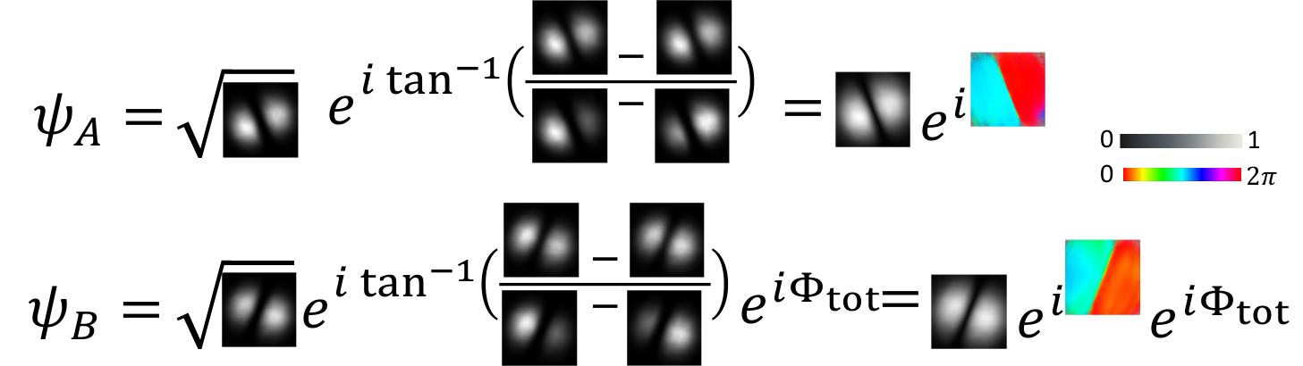
The first step to use these measurements to calculate the total, dynamic, and geometric phases is to use these numerical fields, as produced in Fig. S.1, to find the overlap between the states. This is done as shown below in Eqn. S.8, where we integrate over all of the camera pixels that contain the beam:
| (S.8) |
This is the calculation of , Eqn. 4 of the manuscript.
For the data shown in Fig. S.1, “overlap”, for one set of the five sets of data for that value. Once “overlap” is calculated like this, we find the three respective phases by:
- 1.
Total Phase. For this particular initial condition of :
(S.9) Multiplying by ensures that the total phase remains constantly negative for any value of , to be consistent with the solid-angle definition of geometric phase for partial-circle arcs. (Alternatively, one may simply take modulo at the end for the full-circle results—which is what we’ve invoked to do this.)
For the same example data and same “overlap” above, this results in radians, approximately the expected value of . We double this value to get the phase of the complete circle, radians.
- 2.
Dynamic Phase. Once total phase is found, we can calculate the dynamic phase as shown in Eqn. 7b. Since we have the total phase from the step above, we simply apply Eqn. 6.
(S.10) For the same “overlap” above, the dynamic phase is found to be:
- 3.
Geometric Phase. The geometric phase is then found by:
(S.11) So for the example data shown, , for the complete circle.
All three steps are repeated identically for all 5 measurements for a given angle, and then repeated identically for all angles as shown in Fig. 3 (a). We emphasize that we never invoke explicitly a relationship on the experimental data—the plotted trend in Fig. 3 (a) arises directly from the numerical overlaps of the measured fields detailed above. Lastly, the size of the error bars (for both experiments) are limited by general optical stability of the set-up: floor/table vibrations and slight air turbulence that cause “beam jitters” between one data acquisition and the next.
4. Step-by-Step Experimental Example: Polarization
Firstly, we provide more details comprising the schematic of Fig. 2 (b) in the manuscript. A nm, collimated, single-mode Gaussian is locked to a horizontal polarization with the first linear polarizer (“Lin. Pol.”). A half-waveplate () is used to tune the outgoing intensity of the light to prevent over-saturation on the camera. The beam is sent to a beamsplitter, from which one arm is unmodified to act as reference for total phase measurements. The other arm is sent through another half-waveplate which is mounted in a motorized rotation stage (Thorlabs PRM1Z8 driven by Thorlabs KDC101). This rotation changes the orientation of the waveplate, , which increases on the PS according to .
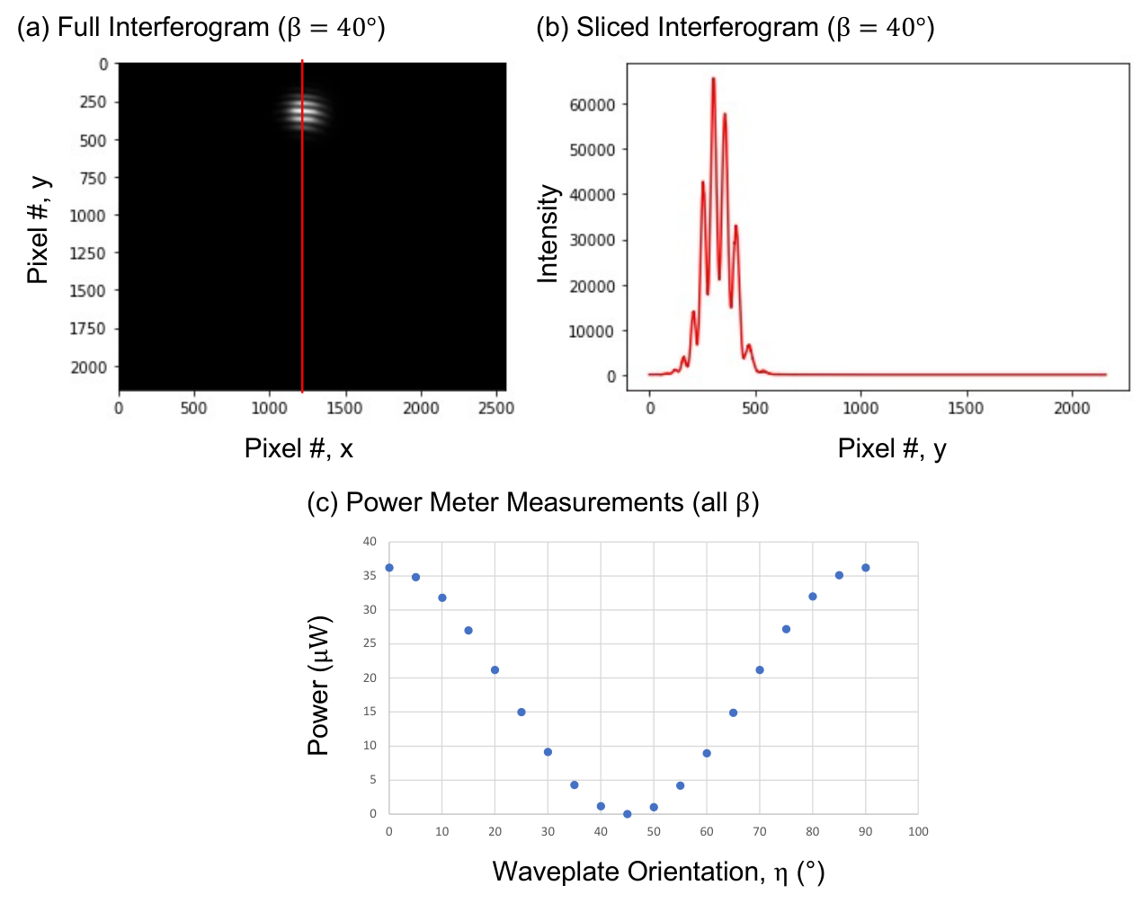
Total phase is measured from the interference between the arms of the interferometer on a camera (Andor Zyla sCMOS), after the beam is reflected back through the half-waveplate to make a complete circle circuit. An example interference pattern is shown in Fig. S.2 (a), where (b) shows the vertical slice used to measure shifts in the fringes. 25 interference images are taken per each set of data.
For each data set (each value), and for each of the 25 images per set, the total phase is extracted by fitting the slice of Fig. S.2 (b) to the following model expression:
| (S.12) |
where the parameters used are: is the intensity, is the background level, is the width of the fringes, is the center location of the Gaussian-envelope with width , and is the sought-after phase shift of the fringes. The average of this phase shift over all 25 images is the desired . We set (the great circle case where there is no dynamic phase), and scale all other total phase measurements to this value.
Once the total phase is measured, the flip mirror is flipped down after the beam makes its first pass through the waveplate (a half-circle is completed on the PS). To measure the dynamic phase, we make a projection measurement on this beam by transmitting it through a linear polarizer locked to the initial polarization of the beam. The result of these measurements, as the waveplate is rotated, is shown in Fig. S.2 (c) which shows the expected trend of Malus law. This is nearly the projection measurement (Eqn. 4 of the manuscript) when we measure the power of the transmitted beam. The polarizer acts on the intensity (rather than the field) of the beam, yielding Malus’s Law: . This data in plotted in Fig. S.2 (c). Thus we modify the power meter measurements to be . The values are then the fractional values of the constant total phase measured previously: . From this, .