Double-layer Kagome Metals $\text{Pt}{\vphantom{\text{X}}}_{\vphantom{\text{2}}\smash[t]{\text{3}}}^{\vphantom{\smash[t]{\text{2}}}\hphantom{\text{3}}\text{}}\text{Tl}{\vphantom{\text{X}}}_{\vphantom{\text{2}}\smash[t]{\text{2}}}^{\vphantom{\smash[t]{\text{2}}}\hphantom{\text{2}}\text{}}$ and $\text{Pt}{\vphantom{\text{X}}}_{\vphantom{\text{2}}\smash[t]{\text{3}}}^{\vphantom{\smash[t]{\text{2}}}\hphantom{\text{3}}\text{}}\text{In}{\vphantom{\text{X}}}_{\vphantom{\text{2}}\smash[t]{\text{2}}}^{\vphantom{\smash[t]{\text{2}}}\hphantom{\text{2}}\text{}}$

The kagome lattice, a 2D network of corner sharing triangles, has played an important role in materials physics for decades. For nearest neighbor antiferromagnetic interactions the lattice provides strong geometrical frustration, and kagome systems became important in the field of frustrated magnetism Ramirez 1994. This naturally led to keen interest in kagome lattice compounds as candidate quantum spin liquids, a key example being herbertsmithite, $\text{ZnCu}{\vphantom{\text{X}}}_{\vphantom{\text{2}}\smash[t]{\text{3}}}^{\vphantom{\smash[t]{\text{2}}}\hphantom{\text{3}}\text{}}\text{(}\text{OH}\text{)}\text{}{\vphantom{\text{X}}}_{\vphantom{\text{2}}\smash[t]{\text{6}}}^{\vphantom{\smash[t]{\text{2}}}\hphantom{\text{6}}\text{}}\text{Cl}{\vphantom{\text{X}}}_{\vphantom{\text{2}}\smash[t]{\text{2}}}^{\vphantom{\smash[t]{\text{2}}}\hphantom{\text{2}}\text{}}$ Shores et al. 2005; Helton et al. 2007; Han et al. 2012; Norman 2016; Mendels and Bert 2016. Quite recently, renewed interest in the kagome lattice has been sparked by its relatively simple but physics-rich electronic structure. The lattice symmetry and connectivity produce Dirac nodes, van Hove singularities, and flat bands. Notably, the flat bands are a result of frustrated electron hopping, reminiscent of the frustrated antiferromagnetic interactions the lattice hosts. Thus, kagome compounds provide model systems to explore the effects of these electronic structure features on a material’s behavior when the Fermi level is located near them. Two clear motivations are the study of electronic topology and the effects of the large density of states associated with the flat band. Topological and Chern insulating behavior is expected under certain circumstances Guo and Franz 2009; Sun et al. 2011; Okamoto et al. 2022, and flat bands may provide a way of generating strong electron-electron interactions and correlated ground states Balents et al. 2020; Sales et al. 2022.

Of particular relevance to the present study are the binary intermetallic compounds containing kagome layers like that shown in Figure 1c, typically made up of a transition metal M (on the kagome net) and a main group metal X Sales et al. 2019; Kang et al. 2020. If these $M_{3}X$ layers are simply stacked the $\text{Mg}{\vphantom{\text{X}}}_{\vphantom{\text{2}}\smash[t]{\text{3}}}^{\vphantom{\smash[t]{\text{2}}}\hphantom{\text{3}}\text{}}\text{Cd}$ structure type is realized. This structure type is adopted by many compounds, including the high temperature ferromagnets $\text{Fe}{\vphantom{\text{X}}}_{\vphantom{\text{2}}\smash[t]{\text{3}}}^{\vphantom{\smash[t]{\text{2}}}\hphantom{\text{3}}\text{}}\text{Sn}$ and $\text{Fe}{\vphantom{\text{X}}}_{\vphantom{\text{2}}\smash[t]{\text{3}}}^{\vphantom{\smash[t]{\text{2}}}\hphantom{\text{3}}\text{}}\text{Ge}$ Jannin et al. 1963; Sales et al. 2014; Kanematsu et al. 1963; McGuire et al. 2018 and chiral antiferromagnets $\text{Mn}{\vphantom{\text{X}}}_{\vphantom{\text{2}}\smash[t]{\text{3}}}^{\vphantom{\smash[t]{\text{2}}}\hphantom{\text{3}}\text{}}\text{Sn}$ and $\text{Mn}{\vphantom{\text{X}}}_{\vphantom{\text{2}}\smash[t]{\text{3}}}^{\vphantom{\smash[t]{\text{2}}}\hphantom{\text{3}}\text{}}\text{Ge}$ Yang et al. 2017; Liu and Balents 2017; Nayak et al. 2016. Alternating these kagome layers with honeycomb layers of the main group element (Figure 1d) results in the CoSn structure type in which the kagome nets are isolated from one another. Examples include FeGe, FeSn, CoSn, NiIn, RhPb, and PtTl, and these compounds have been studied in the context of flat bands, magnetism, and topology Sales et al. 2019; Kang et al. 2020; Meier et al. 2019; Meier et al. 2020; Teng et al. 2022; Teng et al. 2023. Materials with a third type of stacking have also received recent attention, those with two adjacent kagome layers separated by single honeycomb layers. This structure type is represented by two materials: the topologically nontrivial high temperature ferromagnet $\text{Fe}{\vphantom{\text{X}}}_{\vphantom{\text{2}}\smash[t]{\text{3}}}^{\vphantom{\smash[t]{\text{2}}}\hphantom{\text{3}}\text{}}\text{Sn}{\vphantom{\text{X}}}_{\vphantom{\text{2}}\smash[t]{\text{2}}}^{\vphantom{\smash[t]{\text{2}}}\hphantom{\text{2}}\text{}}$ Fenner et al. 2009; Kida et al. 2011; Ye et al. 2018 and the compound $\text{V}{\vphantom{\text{X}}}_{\vphantom{\text{2}}\smash[t]{\text{3}}}^{\vphantom{\smash[t]{\text{2}}}\hphantom{\text{3}}\text{}}\text{Sb}{\vphantom{\text{X}}}_{\vphantom{\text{2}}\smash[t]{\text{2}}}^{\vphantom{\smash[t]{\text{2}}}\hphantom{\text{2}}\text{}}$, which undergoes a density wave transition near 160 K Wang et al. 2022. Recently several Ti-based compounds of this type were predicted theoretically Yi et al. 2023.

There is, in addition, the $\text{Pt}{\vphantom{\text{X}}}_{\vphantom{\text{2}}\smash[t]{\text{3}}}^{\vphantom{\smash[t]{\text{2}}}\hphantom{\text{3}}\text{}}\text{Tl}{\vphantom{\text{X}}}_{\vphantom{\text{2}}\smash[t]{\text{2}}}^{\vphantom{\smash[t]{\text{2}}}\hphantom{\text{2}}\text{}}$ structure type, a variant of the $\text{Fe}{\vphantom{\text{X}}}_{\vphantom{\text{2}}\smash[t]{\text{3}}}^{\vphantom{\smash[t]{\text{2}}}\hphantom{\text{3}}\text{}}\text{Sn}{\vphantom{\text{X}}}_{\vphantom{\text{2}}\smash[t]{\text{2}}}^{\vphantom{\smash[t]{\text{2}}}\hphantom{\text{2}}\text{}}$ structure with the same stacking sequence but a distinct stacking arrangement (Figures 1e and 1f). This structure is adopted by $\text{Pt}{\vphantom{\text{X}}}_{\vphantom{\text{2}}\smash[t]{\text{3}}}^{\vphantom{\smash[t]{\text{2}}}\hphantom{\text{3}}\text{}}\text{Tl}{\vphantom{\text{X}}}_{\vphantom{\text{2}}\smash[t]{\text{2}}}^{\vphantom{\smash[t]{\text{2}}}\hphantom{\text{2}}\text{}}$ and $\text{Pt}{\vphantom{\text{X}}}_{\vphantom{\text{2}}\smash[t]{\text{3}}}^{\vphantom{\smash[t]{\text{2}}}\hphantom{\text{3}}\text{}}\text{In}{\vphantom{\text{X}}}_{\vphantom{\text{2}}\smash[t]{\text{2}}}^{\vphantom{\smash[t]{\text{2}}}\hphantom{\text{2}}\text{}}$. The structures of these compounds were reported more than fifty years ago Bhan et al. 1968, but no information about their electronic or magnetic properties were found in the literature. Here we examine the behavior of these two compounds using x-ray and neutron diffraction, density functional theory, and electrical transport, magnetization, and heat capacity measurements. We find that the Fermi level resides in a pseudo-gap in the density of states, and this theoretical result is in good agreement with our heat capacity and magnetization data. Multiple bands and carrier types appear to contribute to the conduction based on the calculated electronic structure and measured Hall effect. Due in part to the low density of states, we observe diamagnetic behavior, and we see no signature of phase transitions of any kind between room temperature and 2 K. The anisotropic magnetoresistance in $\text{Pt}{\vphantom{\text{X}}}_{\vphantom{\text{2}}\smash[t]{\text{3}}}^{\vphantom{\smash[t]{\text{2}}}\hphantom{\text{3}}\text{}}\text{Tl}{\vphantom{\text{X}}}_{\vphantom{\text{2}}\smash[t]{\text{2}}}^{\vphantom{\smash[t]{\text{2}}}\hphantom{\text{2}}\text{}}$ at 2 K, longitudinal and transverse, shows no sign of saturation up to 13.5 T and reach values exceeding 200%. The longitudinal magnetoresistance shows quantum oscillations (Shubnikov-de Haas oscillations), which are also seen in isothermal magnetization data (de Haas-van Alphen oscillations), indicating reasonably high mobility carriers in the materials.

Starting materials were Pt tubes and sheets (Refining Systems, 99.9%), In shot (Alfa Aesar99.999%) and Tl rods (Alfa Aesar 99.99%). The Pt was cut into 1-2 mm-sized pieces before use to reduce time to react/dissolve during the syntheses. The In was used as received. The Tl was stored, cut, and weighted inside a He or Ar filled glove box to minimize oxidation. Note that Tl is toxic and should be handled with care to prevent exposure. All reactions were performed in alumina crucibles sealed inside fused silica ampoules under vacuum.

$\text{Pt}{\vphantom{\text{X}}}_{\vphantom{\text{2}}\smash[t]{\text{3}}}^{\vphantom{\smash[t]{\text{2}}}\hphantom{\text{3}}\text{}}\text{Tl}{\vphantom{\text{X}}}_{\vphantom{\text{2}}\smash[t]{\text{2}}}^{\vphantom{\smash[t]{\text{2}}}\hphantom{\text{2}}\text{}}$ decomposes peritectically at 900 ^∘C. Single crystals of $\text{Pt}{\vphantom{\text{X}}}_{\vphantom{\text{2}}\smash[t]{\text{3}}}^{\vphantom{\smash[t]{\text{2}}}\hphantom{\text{3}}\text{}}\text{Tl}{\vphantom{\text{X}}}_{\vphantom{\text{2}}\smash[t]{\text{2}}}^{\vphantom{\smash[t]{\text{2}}}\hphantom{\text{2}}\text{}}$ were grown using the self-flux technique based on the published Pt-Tl binary phase diagram Okamoto 1990. Pt and Tl were loaded into a Canfield crucible set Canfield et al. 2016 in a 45:55 molar ratio. At this ratio, the liquidus is near 880 ^∘C. $\text{Pt}{\vphantom{\text{X}}}_{\vphantom{\text{2}}\smash[t]{\text{3}}}^{\vphantom{\smash[t]{\text{2}}}\hphantom{\text{3}}\text{}}\text{Tl}{\vphantom{\text{X}}}_{\vphantom{\text{2}}\smash[t]{\text{2}}}^{\vphantom{\smash[t]{\text{2}}}\hphantom{\text{2}}\text{}}$ is in equilibrium with the liquid down to 752 ^∘C, at which point PtTl begins to precipitate. The reaction was heated over about 4 h to 950 ^∘C, held at this temperature for 48 h to obtain a homogeneous melt, cooled to 800 ^∘C at a rate of 2.3 ^∘C/h, then inverted into a centrifuge to separate the $\text{Pt}{\vphantom{\text{X}}}_{\vphantom{\text{2}}\smash[t]{\text{3}}}^{\vphantom{\smash[t]{\text{2}}}\hphantom{\text{3}}\text{}}\text{Tl}{\vphantom{\text{X}}}_{\vphantom{\text{2}}\smash[t]{\text{2}}}^{\vphantom{\smash[t]{\text{2}}}\hphantom{\text{2}}\text{}}$ crystals from the liquid phase. Figure 1a shows a crystal grown in this way. Polycrystalline $\text{Pt}{\vphantom{\text{X}}}_{\vphantom{\text{2}}\smash[t]{\text{3}}}^{\vphantom{\smash[t]{\text{2}}}\hphantom{\text{3}}\text{}}\text{Tl}{\vphantom{\text{X}}}_{\vphantom{\text{2}}\smash[t]{\text{2}}}^{\vphantom{\smash[t]{\text{2}}}\hphantom{\text{2}}\text{}}$ was synthesized by first heating a stoichiometric mixture of the elements to 850 ^∘C for several days, then 1080 ^∘C for several hours. The sample was removed from the hot furnace into lab air to cool, then heated to 850 ^∘C and held for five days. The sample was then ground, pressed into a pellet, and annealed at 850 ^∘C for five days.

The Pt-In binary phase diagram is significantly more complicated than the Pt-Tl phase diagram Okamoto 1990. $\text{Pt}{\vphantom{\text{X}}}_{\vphantom{\text{2}}\smash[t]{\text{3}}}^{\vphantom{\smash[t]{\text{2}}}\hphantom{\text{3}}\text{}}\text{In}{\vphantom{\text{X}}}_{\vphantom{\text{2}}\smash[t]{\text{2}}}^{\vphantom{\smash[t]{\text{2}}}\hphantom{\text{2}}\text{}}$ is reported to be stable only below a peritectoid reaction at 550 ^∘C. Thus, crystals are not attainable by self-flux techniques, and only polycrystalline $\text{Pt}{\vphantom{\text{X}}}_{\vphantom{\text{2}}\smash[t]{\text{3}}}^{\vphantom{\smash[t]{\text{2}}}\hphantom{\text{3}}\text{}}\text{In}{\vphantom{\text{X}}}_{\vphantom{\text{2}}\smash[t]{\text{2}}}^{\vphantom{\smash[t]{\text{2}}}\hphantom{\text{2}}\text{}}$ is studied here. This was made by reacting a stoichiometric mixture of the elements to 1050 ^∘C for 3 days, then 525 ^∘C for 6 days. Unreacted Pt was noted when grinding the product, so the sample was heated to 1100 ^∘C for two days then quenched in water. The sample was then ground, pelletized, and annealed at 525 ^∘C for one week.

Powder x-ray diffraction data were collected using a PANalytical X’Pert Pro MPD with monochromatic Cu $K_{\alpha 1}$ radiation in the Bragg-Brentano geometry. The neutron diffraction experiment was conducted on the time-of-flight powder diffractometer, POWGEN, located at the Spallation Neutron Source of the Oak Ridge National Laboratory Huq et al. 2011; Huq et al. 2019. The sample environment adopted was a POWGEN Automatic Changer. Approximately 1.1 g of powder sample was loaded into a 6 mm diameter vanadium can filled with helium gas. Neutron bank with center wavelength of 1.5 Å was employed to collect the high-resolution neutron diffraction data covering a Q range of 0.48$-$12.9 Å^-1. FullProf was used for Rietveld refinement of x-ray and neutron diffraction data Rodriguez-Carvajal 1993. Energy dispersive spectroscopy (EDS) was performed using a Bruker Quantax 70 detector with a Hitachi TM3000 scanning electron microscope for semiquantitative chemical analysis.

Magnetization, electrical transport, and heat capacity data were measured using commercial cryostats from Quantum Design (PPMS, MPMS-3, Dyancool). For magnetization measurements, both Vibrating Sample Magnetometer and DC SQUID options from Quantum Design were used. For electrical transport (resistivity, Hall effect, and magnetoresistivity), Resistivity and AC-Transport options from Quantum Design were used. Electrical contacts to the samples were made using silver paste and platinum wires. All transport measurements were done with four contact points, and 2-point resistances between leads were confirmed to be $\sim 1\Omega$ before measurements, and contacts were separated by distances on the order of 1 mm. Heat capacity was measured using the relaxation method with samples mounted using Apiezon N-grease. Property measurements vs temperature were done on cooling. Isothermal magnetization measurements were done starting from the maximum positive fields. Magnetoresistance and Hall effect data were measured from maximum positive field to maximum negative field and then back to maximum positive field. The data were then appropriately symmetrized or antisymmetrized to remove offset voltages and voltages arising from misalignment of the contacts.

To gain insight into the electronic properties of Pt₃In₂ and Pt₃Tl₂, we carried out density functional theory (DFT) calculations using the Vienna Ab initio Simulation Package (VASP) Kresse and Furthmüller 1996; Kresse and Joubert 1999, which uses the projector augmented wave (PAW) approach Blöchl 1994 with the generalized gradient approximation in the parametrization of Perdew, Burke, and Ernzerhof Perdew et al. 1996 for exchange correlation. Throughout the DFT calculations, the spin-orbit coupling was turned on. To calculate the electronic ground state of these compounds, we used the structural data obtained in this work (space group # 194: $P6_{3}/mmc$), a regular $12\times 12\times 6$ $\rm\bf k$-point mesh centered at the $\Gamma$ point, an energy convergence criterion $10^{-6}$ eV, and an energy cutoff $500$ eV. For Pt, we used a standard PAW potential (Pt in the VASP distribution), while for In and Tl we used PAW potentials in which the $d$ semi core states are treated as valence states (In_d and Tl_d in the VASP distribution). After the electronic ground state was obtained, we carried out non-selfconsistent calculations to compute the density of states (DOS) using a denser $20\times 20\times 10$ $\rm\bf k$-point mesh with the smearing parameter $0.1$ eV and the electronic band structure along high-symmetry lines using the optimized charge density.

X-ray diffraction confirmed that the samples adopt the previously reported structures Bhan et al. 1968. This hexagonal structure is illustrated in Figure 1b. It can be decomposed into layers in the ab-plane of composition Pt${}_{3}X$ and of composition $X_{2}$. These layers are shown in Figures 1c and 1d, respectively. The Pt${}_{3}X$ layer contains a kagome net of Pt sites with $X$ atoms at the centers of the hexagonal holes. The $X_{2}$ layer is a honeycomb net. In the full structure, two Pt${}_{3}X$ layers are stacked together, forming a double kagome net of Pt, and these double layers are separated from one another by a single $X_{2}$ layer.

This structure is similar to, but distinct from, the structure of the recently investigated double kagome net compounds $\text{Fe}{\vphantom{\text{X}}}_{\vphantom{\text{2}}\smash[t]{\text{3}}}^{\vphantom{\smash[t]{\text{2}}}\hphantom{\text{3}}\text{}}\text{Sn}{\vphantom{\text{X}}}_{\vphantom{\text{2}}\smash[t]{\text{2}}}^{\vphantom{\smash[t]{\text{2}}}\hphantom{\text{2}}\text{}}$ and $\text{V}{\vphantom{\text{X}}}_{\vphantom{\text{2}}\smash[t]{\text{3}}}^{\vphantom{\smash[t]{\text{2}}}\hphantom{\text{3}}\text{}}\text{Sb}{\vphantom{\text{X}}}_{\vphantom{\text{2}}\smash[t]{\text{2}}}^{\vphantom{\smash[t]{\text{2}}}\hphantom{\text{2}}\text{}}$. The comparison is facilitated by examining Figures 1e and 1f, in which only the transition metal atoms are shown. The different stacking of the double kagome nets is apparent, and nicely illustrates the differences in the compounds’ space group symmetries. In Pt₃X₂ the $6_{3}$ screw axis rotates each double layer around the c-axis by 180^∘ as they are stacked. In the Fe and V compounds, the stacking is defined by the rhombohedral centering, which simply translates each successive layer in the ab-plane relative to the previous layer.

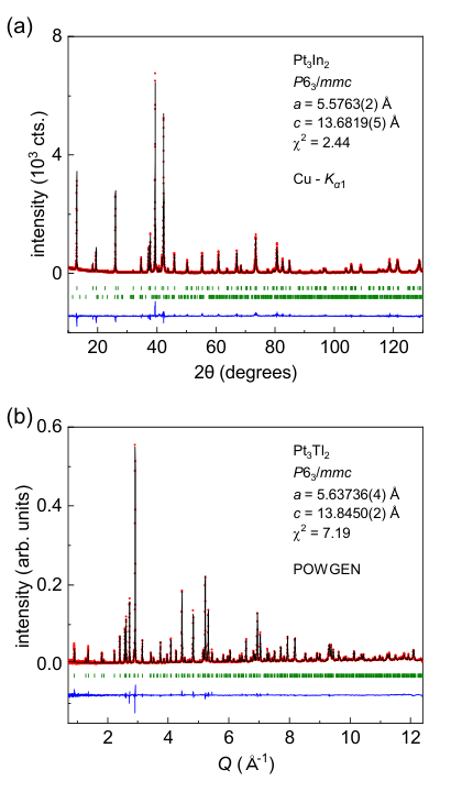
To obtain reliable structural information and investigate the possibility of site disorder in Pt₃X₂, Rietveld refinement of powder diffraction data was performed. Since Pt and In have significantly different atomic numbers, x-ray diffraction is suitable for this. Pt and Tl, however, have little x-ray scattering contrast, so neutron powder diffraction was used for this compound. The results are shown in Figure 2 and structural parameters and agreement indices are summarized in Table 1.

The $\text{Pt}{\vphantom{\text{X}}}_{\vphantom{\text{2}}\smash[t]{\text{3}}}^{\vphantom{\smash[t]{\text{2}}}\hphantom{\text{3}}\text{}}\text{In}{\vphantom{\text{X}}}_{\vphantom{\text{2}}\smash[t]{\text{2}}}^{\vphantom{\smash[t]{\text{2}}}\hphantom{\text{2}}\text{}}$ sample contained a secondary phase identified to be $\text{Pt}{\vphantom{\text{X}}}_{\vphantom{\text{2}}\smash[t]{\text{13}}}^{\vphantom{\smash[t]{\text{2}}}\hphantom{\text{13}}\text{}}\text{In}{\vphantom{\text{X}}}_{\vphantom{\text{2}}\smash[t]{\text{9}}}^{\vphantom{\smash[t]{\text{2}}}\hphantom{\text{9}}\text{}}$. The refinement indicated the concentration of this impurity to be near 3% by weight. The peak shapes indicated the presence of anisotropic strain broadening, likely induced by grinding the sample. This was modeled in FullProf using the quartic form of the general strain formulation in Laue class $6/mmm$ and dramatically improved the fit. The $\text{Pt}{\vphantom{\text{X}}}_{\vphantom{\text{2}}\smash[t]{\text{3}}}^{\vphantom{\smash[t]{\text{2}}}\hphantom{\text{3}}\text{}}\text{Tl}{\vphantom{\text{X}}}_{\vphantom{\text{2}}\smash[t]{\text{2}}}^{\vphantom{\smash[t]{\text{2}}}\hphantom{\text{2}}\text{}}$ sample appeared single phase by neutron diffraction.

The structural parameters are in reasonable agreement with those previously reported Bhan et al. 1968. For both compounds, the refined x coordinate of the Pt atom is within experimental error of 1/6, which corresponds to an ideal kagome net. No evidence for significant site mixing was seen in the data. To test this, refinements were performed with In or Tl mixed onto the Pt site, and separately with Pt mixed onto the three In or Tl sites. For $\text{Pt}{\vphantom{\text{X}}}_{\vphantom{\text{2}}\smash[t]{\text{3}}}^{\vphantom{\smash[t]{\text{2}}}\hphantom{\text{3}}\text{}}\text{In}{\vphantom{\text{X}}}_{\vphantom{\text{2}}\smash[t]{\text{2}}}^{\vphantom{\smash[t]{\text{2}}}\hphantom{\text{2}}\text{}}$, in the former case the composition of the Pt site refined to include only 6% In. In the latter case, refinement returned a maximum amount of Pt on any In site of less than 4%. Neither scenario resulted in an improvement in the fit quality judged by the $\chi^{2}$ values. For $\text{Pt}{\vphantom{\text{X}}}_{\vphantom{\text{2}}\smash[t]{\text{3}}}^{\vphantom{\smash[t]{\text{2}}}\hphantom{\text{3}}\text{}}\text{Tl}{\vphantom{\text{X}}}_{\vphantom{\text{2}}\smash[t]{\text{2}}}^{\vphantom{\smash[t]{\text{2}}}\hphantom{\text{2}}\text{}}$, all the sites refined to their nominal stoichiometric occupancies within the estimated standard deviations, and $\chi^{2}$ was not improved by the site mixings. In addition, the overall average compositions of the two materials were determined by semiquantitative EDS measurements to be Pt_3.0(1)In_2.0(1) and Pt_3.0(1)Tl_2.0(1). This was calculated using spectra from 14 points across multiple $\text{Pt}{\vphantom{\text{X}}}_{\vphantom{\text{2}}\smash[t]{\text{3}}}^{\vphantom{\smash[t]{\text{2}}}\hphantom{\text{3}}\text{}}\text{Tl}{\vphantom{\text{X}}}_{\vphantom{\text{2}}\smash[t]{\text{2}}}^{\vphantom{\smash[t]{\text{2}}}\hphantom{\text{2}}\text{}}$ crystals and single points on 7 different grains of polycrystalline $\text{Pt}{\vphantom{\text{X}}}_{\vphantom{\text{2}}\smash[t]{\text{3}}}^{\vphantom{\smash[t]{\text{2}}}\hphantom{\text{3}}\text{}}\text{In}{\vphantom{\text{X}}}_{\vphantom{\text{2}}\smash[t]{\text{2}}}^{\vphantom{\smash[t]{\text{2}}}\hphantom{\text{2}}\text{}}$. Thus, based on the present study, both $\text{Pt}{\vphantom{\text{X}}}_{\vphantom{\text{2}}\smash[t]{\text{3}}}^{\vphantom{\smash[t]{\text{2}}}\hphantom{\text{3}}\text{}}\text{In}{\vphantom{\text{X}}}_{\vphantom{\text{2}}\smash[t]{\text{2}}}^{\vphantom{\smash[t]{\text{2}}}\hphantom{\text{2}}\text{}}$ and $\text{Pt}{\vphantom{\text{X}}}_{\vphantom{\text{2}}\smash[t]{\text{3}}}^{\vphantom{\smash[t]{\text{2}}}\hphantom{\text{3}}\text{}}\text{Tl}{\vphantom{\text{X}}}_{\vphantom{\text{2}}\smash[t]{\text{2}}}^{\vphantom{\smash[t]{\text{2}}}\hphantom{\text{2}}\text{}}$ appear to be stoichiometric compounds with limited intrinsic disorder.

The calculated electronic structures of $\text{Pt}{\vphantom{\text{X}}}_{\vphantom{\text{2}}\smash[t]{\text{3}}}^{\vphantom{\smash[t]{\text{2}}}\hphantom{\text{3}}\text{}}\text{In}{\vphantom{\text{X}}}_{\vphantom{\text{2}}\smash[t]{\text{2}}}^{\vphantom{\smash[t]{\text{2}}}\hphantom{\text{2}}\text{}}$ and $\text{Pt}{\vphantom{\text{X}}}_{\vphantom{\text{2}}\smash[t]{\text{3}}}^{\vphantom{\smash[t]{\text{2}}}\hphantom{\text{3}}\text{}}\text{Tl}{\vphantom{\text{X}}}_{\vphantom{\text{2}}\smash[t]{\text{2}}}^{\vphantom{\smash[t]{\text{2}}}\hphantom{\text{2}}\text{}}$ are shown in Figure 3. As expected, states within a few eV of the Fermi level are dominated by Pt-$5d$ orbitals, especially the valence bands. In both compounds, multiple bands cross the Fermi level, with several hole-like pockets along the k-path traced in Figure 3a and 3b, and an electron-like pocket near the K point. The Fermi levels lie at pseudogaps in the densities of states (DOS). At $E_{F}$ the total DOS per unit cell (12 Pt aoms, 8 In or Tl atoms) is calculated to be 2.8 eV^-1 for $\text{Pt}{\vphantom{\text{X}}}_{\vphantom{\text{2}}\smash[t]{\text{3}}}^{\vphantom{\smash[t]{\text{2}}}\hphantom{\text{3}}\text{}}\text{In}{\vphantom{\text{X}}}_{\vphantom{\text{2}}\smash[t]{\text{2}}}^{\vphantom{\smash[t]{\text{2}}}\hphantom{\text{2}}\text{}}$ and 1.8 eV^-1 for $\text{Pt}{\vphantom{\text{X}}}_{\vphantom{\text{2}}\smash[t]{\text{3}}}^{\vphantom{\smash[t]{\text{2}}}\hphantom{\text{3}}\text{}}\text{Tl}{\vphantom{\text{X}}}_{\vphantom{\text{2}}\smash[t]{\text{2}}}^{\vphantom{\smash[t]{\text{2}}}\hphantom{\text{2}}\text{}}$.

The flat bands, van Hove singularities, and Dirac nodes characteristic of kagome nets in the tight-binding and nearest-neighbor-hopping limits are not easily identifiable in Pt₃X₂. This is likely due to the extended nature of the Pt-$5d$ orbitals, which results in strong covalent and beyond nearest neighbor interactions. This was similarly seen in CoSn-based compounds with heavier elements Meier et al. 2020, where the these features were much less distinct in PtTl when compared to CoSn and NiIn, or even to the $4d$ transition metal compound RhPb.

Results of electrical resistivity measurements are shown in Figure 4a. The data are plotted relative to values at 300 K. The $\text{Pt}{\vphantom{\text{X}}}_{\vphantom{\text{2}}\smash[t]{\text{3}}}^{\vphantom{\smash[t]{\text{2}}}\hphantom{\text{3}}\text{}}\text{In}{\vphantom{\text{X}}}_{\vphantom{\text{2}}\smash[t]{\text{2}}}^{\vphantom{\smash[t]{\text{2}}}\hphantom{\text{2}}\text{}}$ sample was a piece cut from a polycrystalline pellet that had been pressed and sintered as described in the Materials and Methods section. The sample was small and not ideally shaped for accurately determining the cross sectional area for the current flow. This along with the polycrystalline nature of the sample make any precise value of the resistivity unreliable, but measurements near room temperature suggest the powder-averaged resistivity of $\text{Pt}{\vphantom{\text{X}}}_{\vphantom{\text{2}}\smash[t]{\text{3}}}^{\vphantom{\smash[t]{\text{2}}}\hphantom{\text{3}}\text{}}\text{In}{\vphantom{\text{X}}}_{\vphantom{\text{2}}\smash[t]{\text{2}}}^{\vphantom{\smash[t]{\text{2}}}\hphantom{\text{2}}\text{}}$ is in the $10^{-4}~\Omega$cm range. A $\text{Pt}{\vphantom{\text{X}}}_{\vphantom{\text{2}}\smash[t]{\text{3}}}^{\vphantom{\smash[t]{\text{2}}}\hphantom{\text{3}}\text{}}\text{Tl}{\vphantom{\text{X}}}_{\vphantom{\text{2}}\smash[t]{\text{2}}}^{\vphantom{\smash[t]{\text{2}}}\hphantom{\text{2}}\text{}}$ crystal was used for the measurements, and the current was applied in the ab-plane. The value measured at 300 K was $1.2\times 10^{-4}~\Omega$cm. Both compounds behave like metals with resistivity increasing approximately linearly with temperature above about 50 K. The residual resistivity ratio defined as $R$(300 K)/$R$(2 K) is about 4 for $\text{Pt}{\vphantom{\text{X}}}_{\vphantom{\text{2}}\smash[t]{\text{3}}}^{\vphantom{\smash[t]{\text{2}}}\hphantom{\text{3}}\text{}}\text{In}{\vphantom{\text{X}}}_{\vphantom{\text{2}}\smash[t]{\text{2}}}^{\vphantom{\smash[t]{\text{2}}}\hphantom{\text{2}}\text{}}$ and about 5 for $\text{Pt}{\vphantom{\text{X}}}_{\vphantom{\text{2}}\smash[t]{\text{3}}}^{\vphantom{\smash[t]{\text{2}}}\hphantom{\text{3}}\text{}}\text{Tl}{\vphantom{\text{X}}}_{\vphantom{\text{2}}\smash[t]{\text{2}}}^{\vphantom{\smash[t]{\text{2}}}\hphantom{\text{2}}\text{}}$.

The Hall effect was measured for $\text{Pt}{\vphantom{\text{X}}}_{\vphantom{\text{2}}\smash[t]{\text{3}}}^{\vphantom{\smash[t]{\text{2}}}\hphantom{\text{3}}\text{}}\text{Tl}{\vphantom{\text{X}}}_{\vphantom{\text{2}}\smash[t]{\text{2}}}^{\vphantom{\smash[t]{\text{2}}}\hphantom{\text{2}}\text{}}$ and the results are shown in the inset of Figure 4a. For these measurements the field $H$ was applied out of the plane of the crystal. The data are plotted as $\rho_{yx}=V_{y}t/I_{x}$, where the current $I$ and measured voltage $V$ are in the plane and $t$ is the thickness of the crystal. The observed nonlinearity of $\rho_{yx}$ vs H indicates the contribution from both electron and hole bands to the conduction. The Hall effect changes strongly with temperature as well, with the low field Hall coefficient changing sign between 100 and 2 K.

The Hall effect data suggest a relatively complex Fermi surface, with the contributions from multiple carrier pockets changing with temperature. The resistivity data are consistent with typical behaviors seen in “bad” metals, semi-metals, or degenerately doped semiconductors. Both of these observations are consistent with the calculated electronic structures discussed above, which show the Fermi level resides in a pseudo-gap region but is crossed by multiple bands.

The heat capacity is shown in Figure 4b. The data show no indications of phase transitions, consistent with the transport results discussed above and the magnetization data below. At high temperatures the specific heat capacities ($c_{P}$) per mole of formula unit (f.u.) approach the Dulong-Petit limit of 3R per mole of atoms or 124.7 J mol-f.u.^-1K^-2. The low temperature behavior is shown in the inset of Figure 4b, with the data plotted as $c_{P}/T$ vs $T^{2}$. The linear fits shown on the plot give the Sommerfeld coefficient $\gamma$ from the intercept and the Debye temperature $\theta_{D}$ can be determined from the slope. For $\text{Pt}{\vphantom{\text{X}}}_{\vphantom{\text{2}}\smash[t]{\text{3}}}^{\vphantom{\smash[t]{\text{2}}}\hphantom{\text{3}}\text{}}\text{In}{\vphantom{\text{X}}}_{\vphantom{\text{2}}\smash[t]{\text{2}}}^{\vphantom{\smash[t]{\text{2}}}\hphantom{\text{2}}\text{}}$ this gives $\gamma$ = 2.0(2) mJ mol-f.u.^-1K^-2 and $\theta_{D}$ = 254(6) K. For the $\text{Pt}{\vphantom{\text{X}}}_{\vphantom{\text{2}}\smash[t]{\text{3}}}^{\vphantom{\smash[t]{\text{2}}}\hphantom{\text{3}}\text{}}\text{Tl}{\vphantom{\text{X}}}_{\vphantom{\text{2}}\smash[t]{\text{2}}}^{\vphantom{\smash[t]{\text{2}}}\hphantom{\text{2}}\text{}}$ crystal this gives $\gamma$ = 0.52(5) mJ mol-f.u.^-1K^-2 and $\theta_{D}$ = 218(1) K. The polycrystalline sample of $\text{Pt}{\vphantom{\text{X}}}_{\vphantom{\text{2}}\smash[t]{\text{3}}}^{\vphantom{\smash[t]{\text{2}}}\hphantom{\text{3}}\text{}}\text{Tl}{\vphantom{\text{X}}}_{\vphantom{\text{2}}\smash[t]{\text{2}}}^{\vphantom{\smash[t]{\text{2}}}\hphantom{\text{2}}\text{}}$ used for neutron diffraction was also measured, and gave similar values of $\gamma$ = 0.5(2) mJ mol-f.u.^-1K^-2 and $\theta_{D}$ = 213(4) K. The Debye temperatures are relatively low, consistent with the heavy element constituents, and as expected somewhat higher in the In compound than the Tl compound. Note that the inset in Figure 4b contains data collected in zero field (used for the linear fitting) and also in relatively high applied magnetic fields. The results show no significant magnetic field effect on the heat capacity.

Comparing the values of $\gamma$ between the two compounds indicates a higher electronic density of states at the Fermi level in $\text{Pt}{\vphantom{\text{X}}}_{\vphantom{\text{2}}\smash[t]{\text{3}}}^{\vphantom{\smash[t]{\text{2}}}\hphantom{\text{3}}\text{}}\text{In}{\vphantom{\text{X}}}_{\vphantom{\text{2}}\smash[t]{\text{2}}}^{\vphantom{\smash[t]{\text{2}}}\hphantom{\text{2}}\text{}}$ than in $\text{Pt}{\vphantom{\text{X}}}_{\vphantom{\text{2}}\smash[t]{\text{3}}}^{\vphantom{\smash[t]{\text{2}}}\hphantom{\text{3}}\text{}}\text{Tl}{\vphantom{\text{X}}}_{\vphantom{\text{2}}\smash[t]{\text{2}}}^{\vphantom{\smash[t]{\text{2}}}\hphantom{\text{2}}\text{}}$. This is supported by the electronic structure calculations in Figure 3, and may partially explain why the resistivity values in the two samples are similar despite the polycrystalline nature of the $\text{Pt}{\vphantom{\text{X}}}_{\vphantom{\text{2}}\smash[t]{\text{3}}}^{\vphantom{\smash[t]{\text{2}}}\hphantom{\text{3}}\text{}}\text{In}{\vphantom{\text{X}}}_{\vphantom{\text{2}}\smash[t]{\text{2}}}^{\vphantom{\smash[t]{\text{2}}}\hphantom{\text{2}}\text{}}$ sample. The Sommerfeld coefficient can be calculated from the DOS at $E_{F}$ [$D(E_{F})$] by $\gamma=(\pi^{2}/3)k_{B}^{2}D(E_{F})$. Using $D(E_{F})$ = 0.70 eV^-1f.u.^-1 and 0.45 eV^-1f.u.^-1 for the In and Tl compounds, respectively, gives $\gamma$($\text{Pt}{\vphantom{\text{X}}}_{\vphantom{\text{2}}\smash[t]{\text{3}}}^{\vphantom{\smash[t]{\text{2}}}\hphantom{\text{3}}\text{}}\text{In}{\vphantom{\text{X}}}_{\vphantom{\text{2}}\smash[t]{\text{2}}}^{\vphantom{\smash[t]{\text{2}}}\hphantom{\text{2}}\text{}}$) = 1.7 mJ K²f.u.^-1 and $\gamma$($\text{Pt}{\vphantom{\text{X}}}_{\vphantom{\text{2}}\smash[t]{\text{3}}}^{\vphantom{\smash[t]{\text{2}}}\hphantom{\text{3}}\text{}}\text{Tl}{\vphantom{\text{X}}}_{\vphantom{\text{2}}\smash[t]{\text{2}}}^{\vphantom{\smash[t]{\text{2}}}\hphantom{\text{2}}\text{}}$) = 1.1 mJ K²f.u.^-1. These values are similar to those extracted from the low temperature heat capacity data, and the similarities suggest the compounds have relatively weak electron-electron correlations.

The magnetic behaviors are summarized in Figure 5. The main panel shows the magnetic susceptibility of single crystals of $\text{Pt}{\vphantom{\text{X}}}_{\vphantom{\text{2}}\smash[t]{\text{3}}}^{\vphantom{\smash[t]{\text{2}}}\hphantom{\text{3}}\text{}}\text{Tl}{\vphantom{\text{X}}}_{\vphantom{\text{2}}\smash[t]{\text{2}}}^{\vphantom{\smash[t]{\text{2}}}\hphantom{\text{2}}\text{}}$ measured with the field applied parallel and perpendicular to the crystallographic c-axis and of polycrystalline $\text{Pt}{\vphantom{\text{X}}}_{\vphantom{\text{2}}\smash[t]{\text{3}}}^{\vphantom{\smash[t]{\text{2}}}\hphantom{\text{3}}\text{}}\text{In}{\vphantom{\text{X}}}_{\vphantom{\text{2}}\smash[t]{\text{2}}}^{\vphantom{\smash[t]{\text{2}}}\hphantom{\text{2}}\text{}}$. The data have been corrected to account for contributions from the sample holders. All of the data sets contain Curie tails, low temperature upturns upon cooling, that may be attributed to low concentrations of local moments associated with defects or impurities. Otherwise, the data are negative and relatively temperature independent (some weak but notable $T$ dependence is seen for $H$ along the c-axis in $\text{Pt}{\vphantom{\text{X}}}_{\vphantom{\text{2}}\smash[t]{\text{3}}}^{\vphantom{\smash[t]{\text{2}}}\hphantom{\text{3}}\text{}}\text{Tl}{\vphantom{\text{X}}}_{\vphantom{\text{2}}\smash[t]{\text{2}}}^{\vphantom{\smash[t]{\text{2}}}\hphantom{\text{2}}\text{}}$).

Estimating the core or Larmor diamagnetic contribution using the values tabulated for the noble gas cores in Ref. 41 gives $-1.9\times 10^{-4}$ cm³mol-f.u.^-1 for $\text{Pt}{\vphantom{\text{X}}}_{\vphantom{\text{2}}\smash[t]{\text{3}}}^{\vphantom{\smash[t]{\text{2}}}\hphantom{\text{3}}\text{}}\text{In}{\vphantom{\text{X}}}_{\vphantom{\text{2}}\smash[t]{\text{2}}}^{\vphantom{\smash[t]{\text{2}}}\hphantom{\text{2}}\text{}}$ and $-2.2\times 10^{-4}$ cm³mol-f.u.^-1 for $\text{Pt}{\vphantom{\text{X}}}_{\vphantom{\text{2}}\smash[t]{\text{3}}}^{\vphantom{\smash[t]{\text{2}}}\hphantom{\text{3}}\text{}}\text{Tl}{\vphantom{\text{X}}}_{\vphantom{\text{2}}\smash[t]{\text{2}}}^{\vphantom{\smash[t]{\text{2}}}\hphantom{\text{2}}\text{}}$. The remaining magnetism is attributed to the conduction electrons. This includes Landau diamagnetism due to electronic orbits and Pauli paramagnetism due to electron spin. Both are proportional to the density of states at the Fermi level. For a band with effective mass $m*$, this magnetic susceptibility is given by $\chi_{0}=\mu_{B}^{2}D(E_{F})[1-\frac{1}{3}(m_{e}/m*)^{2}]$, where the first term is the Pauli contribution and the second the Landau contribution. Since the Landau diamagnetism depends on the effective mass, it can overcome the positive Pauli contribution if the effective mass is small (less than $m_{e}/\sqrt{3}$ for a spherical Fermi surface) Blundell 2001. It can also be anisotropic, and may account for the anisotropic behavior seen for $\text{Pt}{\vphantom{\text{X}}}_{\vphantom{\text{2}}\smash[t]{\text{3}}}^{\vphantom{\smash[t]{\text{2}}}\hphantom{\text{3}}\text{}}\text{Tl}{\vphantom{\text{X}}}_{\vphantom{\text{2}}\smash[t]{\text{2}}}^{\vphantom{\smash[t]{\text{2}}}\hphantom{\text{2}}\text{}}$ in Figure 5 and in some related CoSn-type kagome compounds Meier et al. 2020.

The expected temperature independent susceptibility from the conduction electrons can be estimated using $D(E_{F})$ values determined from the DFT calculations and assuming an effective mass of unity so that $\chi_{0}=\frac{2}{3}\mu_{B}^{2}D(E_{F})$. In this case the combined Pauli and Landau susceptibility $\chi_{0}$ (in units of cm³mol-f.u.^-1) is calculated from $D(E_{F})$ in units of eV^-1f.u.^-1 by $\chi_{0}=2.15\times 10^{-5}D(E_{F})$. This gives 1.5$\times 10^{-5}$ cm³mol-f.u.^-1 for $\text{Pt}{\vphantom{\text{X}}}_{\vphantom{\text{2}}\smash[t]{\text{3}}}^{\vphantom{\smash[t]{\text{2}}}\hphantom{\text{3}}\text{}}\text{In}{\vphantom{\text{X}}}_{\vphantom{\text{2}}\smash[t]{\text{2}}}^{\vphantom{\smash[t]{\text{2}}}\hphantom{\text{2}}\text{}}$ and 9.7$\times 10^{-6}$ cm³mol-f.u.^-1 for $\text{Pt}{\vphantom{\text{X}}}_{\vphantom{\text{2}}\smash[t]{\text{3}}}^{\vphantom{\smash[t]{\text{2}}}\hphantom{\text{3}}\text{}}\text{Tl}{\vphantom{\text{X}}}_{\vphantom{\text{2}}\smash[t]{\text{2}}}^{\vphantom{\smash[t]{\text{2}}}\hphantom{\text{2}}\text{}}$.

The above estimates of the Larmor susceptibility calculated from the noble gas cores and the Pauli + Landau contributions calculated from $D(E_{F})$ can be combined for comparison with the measured values in Figure 5. The calculated total susceptibility for $\text{Pt}{\vphantom{\text{X}}}_{\vphantom{\text{2}}\smash[t]{\text{3}}}^{\vphantom{\smash[t]{\text{2}}}\hphantom{\text{3}}\text{}}\text{In}{\vphantom{\text{X}}}_{\vphantom{\text{2}}\smash[t]{\text{2}}}^{\vphantom{\smash[t]{\text{2}}}\hphantom{\text{2}}\text{}}$ is $-1.8\times 10^{-4}$ cm³mol-f.u.^-1, and the measured value at room temperature is $-2.2\times 10^{-4}$ cm³mol-f.u.^-1. The calculated value for $\text{Pt}{\vphantom{\text{X}}}_{\vphantom{\text{2}}\smash[t]{\text{3}}}^{\vphantom{\smash[t]{\text{2}}}\hphantom{\text{3}}\text{}}\text{Tl}{\vphantom{\text{X}}}_{\vphantom{\text{2}}\smash[t]{\text{2}}}^{\vphantom{\smash[t]{\text{2}}}\hphantom{\text{2}}\text{}}$ is $-2.1\times 10^{-4}$ cm³mol-f.u.^-1. This should be compared to the isotropic average of the measured susceptibility given by $[2\chi(H\perp c)+\chi(H\|c)]/3$, which is $-2.6\times 10^{-4}$ cm³mol-f.u.^-1 at room temperature. Considering the approximations and assumptions, the calculated and experimental values compare quite favorably.

Since single crystals of $\text{Pt}{\vphantom{\text{X}}}_{\vphantom{\text{2}}\smash[t]{\text{3}}}^{\vphantom{\smash[t]{\text{2}}}\hphantom{\text{3}}\text{}}\text{Tl}{\vphantom{\text{X}}}_{\vphantom{\text{2}}\smash[t]{\text{2}}}^{\vphantom{\smash[t]{\text{2}}}\hphantom{\text{2}}\text{}}$ were available, anistropic magnetoresistance measurements were performed at 2 K and fields up to $\pm$13.5 T. For these measurements, the current $I$ was always applied in the plane of the platelike crystals ($I\perp c$). The field was applied in three directions relative to the current and the crystal. The longitudinal magnetoresistance (L-MR) was measured by applying the field parallel to the current ($H\|I$). The transverse magnetoresistance (T-MR) was measured by applying the field perpendicular to the current ($H\perp I$), with the field directed either out of the plane ($H\|c$) or in the plane ($H\perp c$). The measurements were performed at 2 K and the results are summarized in Figure 6.

Each magnetoresistance curve shows interesting behaviors. The T-MR for $H\|c$ reaches a remarkably high value of 204% with no indication of saturation. The T-MR with $H\perp c$ is approximately linear for fields above a few Tesla, and also reaches a high value of 65%. Large magnetoresistance is often associated with high carrier mobility and/or semimetallike band structures with nearly compensated electron and hole pockets Ali et al. 2014. The latter may apply to $\text{Pt}{\vphantom{\text{X}}}_{\vphantom{\text{2}}\smash[t]{\text{3}}}^{\vphantom{\smash[t]{\text{2}}}\hphantom{\text{3}}\text{}}\text{Tl}{\vphantom{\text{X}}}_{\vphantom{\text{2}}\smash[t]{\text{2}}}^{\vphantom{\smash[t]{\text{2}}}\hphantom{\text{2}}\text{}}$ based on the band structure and properties described above.

The most remarkable features in the data are the undulations seen in the L-MR at high fields. This is shown in Figure 6b, where data measured on two different crystals are plotted. These are interpreted as quantum oscillations arising from the Shubnikov–de Haas effect, where the frequency of the oscillations (in 1/$\mu_{0}H$) relate to the area of closed extremal orbits on the Fermi surface Shoenberg 1984. These oscillations are not as easily observed in magnetoresistance data in other orientations, likely because of the overall larger field dependence of the resistivity in those cases.

A quadratic background was fit to the L-MR data from 4 to 13.5 T and then subtracted to reveal the oscillatory nature. This is shown in Figure 7a, where the background subtracted data is plotted as a function of inverse magnetic field. The same physics that produces the Shubnikov–de Haas effect in transport data is expected to produce the de Haas-van Alphen effect in magnetization Shoenberg 1984. Therefore, the isothermal magnetization curve measured at 2 K with $H\perp c$ was similarly examined. The resulting field dependence is plotted in Figure 7a and it matches well the oscillations in resistivity. Three local maxima can be seen in the resistance data, at 0.086, 0.122, and about 0.16 T^-1. From this an approximate frequency of 27 T can be estimated. The magnetization of $\text{Pt}{\vphantom{\text{X}}}_{\vphantom{\text{2}}\smash[t]{\text{3}}}^{\vphantom{\smash[t]{\text{2}}}\hphantom{\text{3}}\text{}}\text{In}{\vphantom{\text{X}}}_{\vphantom{\text{2}}\smash[t]{\text{2}}}^{\vphantom{\smash[t]{\text{2}}}\hphantom{\text{2}}\text{}}$ at 2 K was also examined to see if quantum oscillations could be observed. The results are shown in Figure 7b. Oscillations are indeed seen, with a period of 0.020 T^-1 or frequency of 50 T.

Pt₃X₂ ($X$ = In and Tl) are double-layer kagome metals with structures similar to but distinct from that of the topologically nontrivial high temperature ferromagnet $\text{Fe}{\vphantom{\text{X}}}_{\vphantom{\text{2}}\smash[t]{\text{3}}}^{\vphantom{\smash[t]{\text{2}}}\hphantom{\text{3}}\text{}}\text{Sn}{\vphantom{\text{X}}}_{\vphantom{\text{2}}\smash[t]{\text{2}}}^{\vphantom{\smash[t]{\text{2}}}\hphantom{\text{2}}\text{}}$ and the density wave hosting compound $\text{V}{\vphantom{\text{X}}}_{\vphantom{\text{2}}\smash[t]{\text{3}}}^{\vphantom{\smash[t]{\text{2}}}\hphantom{\text{3}}\text{}}\text{Sb}{\vphantom{\text{X}}}_{\vphantom{\text{2}}\smash[t]{\text{2}}}^{\vphantom{\smash[t]{\text{2}}}\hphantom{\text{2}}\text{}}$. Here we have reported results from our investigation of these materials, including the growth of $\text{Pt}{\vphantom{\text{X}}}_{\vphantom{\text{2}}\smash[t]{\text{3}}}^{\vphantom{\smash[t]{\text{2}}}\hphantom{\text{3}}\text{}}\text{Tl}{\vphantom{\text{X}}}_{\vphantom{\text{2}}\smash[t]{\text{2}}}^{\vphantom{\smash[t]{\text{2}}}\hphantom{\text{2}}\text{}}$ producing large single crystals and a thorough examination of the structures and electronic properties of the two compounds. Our main findings are (1) the materials are stoichiometric with limited site mixing between Pt and In/Tl, (2) no phase transitions are identified between room temperature and 2 K, (3) the Fermi level lies in a pseudogap in the band structure of both compounds, (4) despite the absence of characteristic kagome-related band structure features interesting electronic behaviors are observed, including relatively large, linear, and non-saturating magnetoresistance and quantum oscillations related to the Shubnikov-de Haas and de Haas-van Alphen effects at 2 K in the magnetoresistance and magnetization data, respectively. Because the electronic structures near the Fermi levels are dominated by Pt bands, these behaviors are necessarily related to the kagome networks in the compounds and expand our overall picture and understanding of kagome metal systems.

This research was funded by the U.S. Department of Energy, Office of Science, Basic Energy Sciences, Materials Sciences and Engineering Division. This research at ORNL’s Spallation Neutron Source was sponsored by the Scientific User Facilities Division, Office of Basic Energy Sciences, U.S. Department of Energy. This research used resources of the Compute and Data Environment for Science (CADES) at the Oak Ridge National Laboratory, which is supported by the Office of Science of the U.S. Department of Energy under Contract No. DE-AC05-00OR22725.

References

- Ramirez (1994) Ramirez, A. Strongly geometrically frustrated magnets. Annu. Rev. Mater. Sci. 1994, 24, 453–480.
- Shores et al. (2005) Shores, M.P.; Nytko, E.A.; Bartlett, B.M.; Nocera, D.G. A structurally perfect S = 1/2 kagome antiferromagnet. J. Am. Chem. Soc. 2005, 127, 13462–13463.
- Helton et al. (2007) Helton, J.; Matan, K.; Shores, M.; Nytko, E.; Bartlett, B.; Yoshida, Y.; Takano, Y.; Suslov, A.; Qiu, Y.; Chung, J.H.; et al. Spin dynamics of the spin-1/2 kagome lattice antiferromagnet ZnCu3(OH)6Cl2. Phys. Rev. Lett. 2007, 98, 107204.
- Han et al. (2012) Han, T.H.; Helton, J.S.; Chu, S.; Nocera, D.G.; Rodriguez-Rivera, J.A.; Broholm, C.; Lee, Y.S. Fractionalized excitations in the spin-liquid state of a kagome-lattice antiferromagnet. Nature 2012, 492, 406–410.
- Norman (2016) Norman, M. Colloquium: Herbertsmithite and the search for the quantum spin liquid. Rev. Mod. Phys. 2016, 88, 041002.
- Mendels and Bert (2016) Mendels, P.; Bert, F. Quantum kagome frustrated antiferromagnets: One route to quantum spin liquids. C. R. Phys. 2016, 17, 455–470.
- Guo and Franz (2009) Guo, H.M.; Franz, M. Topological insulator on the kagome lattice. Phys. Rev. B 2009, 80, 113102.
- Sun et al. (2011) Sun, K.; Gu, Z.; Katsura, H.; Sarma, S.D. Nearly flatbands with nontrivial topology. Phys. Rev. Lett. 2011, 106, 236803.
- Okamoto et al. (2022) Okamoto, S.; Mohanta, N.; Dagotto, E.; Sheng, D. Topological flat bands in a kagome lattice multiorbital system. Commun. Phys. 2022, 5, 198.
- Balents et al. (2020) Balents, L.; Dean, C.R.; Efetov, D.K.; Young, A.F. Superconductivity and strong correlations in moiré flat bands. Nat. Phys. 2020, 16, 725–733.
- Sales et al. (2022) Sales, B.C.; Meier, W.R.; Parker, D.S.; Yin, L.; Yan, J.; May, A.F.; Calder, S.; Aczel, A.A.; Zhang, Q.; Li, H.; et al. Chemical Control of Magnetism in the Kagome Metal CoSn1-xInx: Magnetic Order from Nonmagnetic Substitutions. Chem. Mater. 2022, 34, 7069–7077.
- Sales et al. (2019) Sales, B.C.; Yan, J.; Meier, W.R.; Christianson, A.D.; Okamoto, S.; McGuire, M.A. Electronic, magnetic, and thermodynamic properties of the kagome layer compound FeSn. Phys. Rev. Mater. 2019, 3, 114203.
- Kang et al. (2020) Kang, M.; Ye, L.; Fang, S.; You, J.S.; Levitan, A.; Han, M.; Facio, J.I.; Jozwiak, C.; Bostwick, A.; Rotenberg, E.; et al. Dirac fermions and flat bands in the ideal kagome metal FeSn. Nat. Mater. 2020, 19, 163–169.
- Jannin et al. (1963) Jannin, C.; Michel, A.; Lecocq, P. Magnetism and properties of different phases in the Fe-Sn system. C. R. Hebd. Séances Acad. Sci. 1963, 257, 1906–1907.
- Sales et al. (2014) Sales, B.C.; Saparov, B.; McGuire, M.A.; Singh, D.J.; Parker, D.S. Ferromagnetism of Fe3Sn and alloys. Sci. Rep. 2014, 4, 1–6.
- Kanematsu et al. (1963) Kanematsu, K.; Ohoyama, T.; et al. Magnetic properties and phase transition of Fe3Ge. J. Phys. Soc. Japan 1963, 18, 920–921.
- McGuire et al. (2018) McGuire, M.A.; Shanavas, K.; Kesler, M.S.; Parker, D.S. Tuning magnetocrystalline anisotropy by cobalt alloying in hexagonal Fe3Ge. Sci. Rep. 2018, 8, 14206.
- Yang et al. (2017) Yang, H.; Sun, Y.; Zhang, Y.; Shi, W.J.; Parkin, S.S.; Yan, B. Topological Weyl semimetals in the chiral antiferromagnetic materials Mn3Ge and Mn3Sn. New J. Phys. 2017, 19, 015008.
- Liu and Balents (2017) Liu, J.; Balents, L. Anomalous Hall effect and topological defects in antiferromagnetic Weyl semimetals: Mn3Sn/Ge. Phys. Rev. Lett. 2017, 119, 087202.
- Nayak et al. (2016) Nayak, A.K.; Fischer, J.E.; Sun, Y.; Yan, B.; Karel, J.; Komarek, A.C.; Shekhar, C.; Kumar, N.; Schnelle, W.; Kübler, J.; et al. Large anomalous Hall effect driven by a nonvanishing Berry curvature in the noncolinear antiferromagnet Mn3Ge. Sci. Adv. 2016, 2, e1501870.
- Meier et al. (2019) Meier, W.R.; Yan, J.; McGuire, M.A.; Wang, X.; Christianson, A.D.; Sales, B.C. Reorientation of antiferromagnetism in cobalt doped FeSn. Phys. Rev. B 2019, 100, 184421.
- Meier et al. (2020) Meier, W.R.; Du, M.H.; Okamoto, S.; Mohanta, N.; May, A.F.; McGuire, M.A.; Bridges, C.A.; Samolyuk, G.D.; Sales, B.C. Flat bands in the CoSn-type compounds. Phys. Rev. B 2020, 102, 075148.
- Teng et al. (2022) Teng, X.; Chen, L.; Ye, F.; Rosenberg, E.; Liu, Z.; Yin, J.X.; Jiang, Y.X.; Oh, J.S.; Hasan, M.Z.; Neubauer, K.J.; et al. Discovery of charge density wave in a kagome lattice antiferromagnet. Nature 2022, 609, 490–495.
- Teng et al. (2023) Teng, X.; Oh, J.S.; Tan, H.; Chen, L.; Huang, J.; Gao, B.; Yin, J.X.; Chu, J.H.; Hashimoto, M.; Lu, D.; et al. Magnetism and charge density wave order in kagome FeGe. Nat. Phys. 2023, pp. 1–9.
- Fenner et al. (2009) Fenner, L.; Dee, A.; Wills, A. Non-collinearity and spin frustration in the itinerant kagome ferromagnet Fe3Sn2. J. Phys. Condens. Matter. 2009, 21, 452202.
- Kida et al. (2011) Kida, T.; Fenner, L.; Dee, A.; Terasaki, I.; Hagiwara, M.; Wills, A. The giant anomalous Hall effect in the ferromagnet Fe3Sn2 — a frustrated kagome metal. J. Phys. Condens. Matter. 2011, 23, 112205.
- Ye et al. (2018) Ye, L.; Kang, M.; Liu, J.; Von Cube, F.; Wicker, C.R.; Suzuki, T.; Jozwiak, C.; Bostwick, A.; Rotenberg, E.; Bell, D.C.; et al. Massive Dirac fermions in a ferromagnetic kagome metal. Nature 2018, 555, 638–642.
- Wang et al. (2022) Wang, N.; Gu, Y.; McGuire, M.A.; Yan, J.; Shi, L.; Cui, Q.; Chen, K.; Wang, Y.; Zhang, H.; Yang, H.; et al. A density-wave-like transition in the polycrystalline V3Sb2 sample with bilayer kagome lattice. Chin. Phys. B 2022, 31, 017106.
- Yi et al. (2023) Yi, X.W.; Liao, Z.W.; You, J.Y.; Gu, B.; Su, G. Topological superconductivity and large spin Hall effect in the kagome family Ti (X= Bi, Sb, Pb, Tl, and In). Iscience 2023, 26, 105813.
- Bhan et al. (1968) Bhan, S.; Gödecke, T.; Panday, P.; Schubert, K. Über die mischungen palladium-thallium und platin-thallium. J. Less-Common Met. 1968, 16, 415–425.
- Okamoto (1990) Okamoto, H. Pt-Tl (Platinum-Thallium). Binary Alloy Phase Diagrams, II Ed., Ed. T. B. Massalski 1990, 3, 3143.
- Canfield et al. (2016) Canfield, P.C.; Kong, T.; Kaluarachchi, U.S.; Jo, N.H. Use of frit-disc crucibles for routine and exploratory solution growth of single crystalline samples. Philos. Mag. 2016, 96, 84–92.
- Okamoto (1990) Okamoto, H. In-Pt (Indium-Platinum). Binary Alloy Phase Diagrams, II Ed., Ed. T. B. Massalski 1990, 3, 2276.
- Huq et al. (2011) Huq, A.; Hodges, J.P.; Gourdon, O.; Heroux, L. Powgen: A third-generation high-resolution high-throughput powder diffraction instrument at the Spallation Neutron Source. Z. Kristallogr. Proc. 2011, 1, 127–135.
- Huq et al. (2019) Huq, A.; Kirkham, M.; Peterson, P.F.; Hodges, J.P.; Whitfield, P.S.; Page, K.; Hűgle, T.; Iverson, E.B.; Parizzi, A.; Rennich, G. POWGEN: rebuild of a third-generation powder diffractometer at the Spallation Neutron Source. J. Appl. Crystallogr. 2019, 52, 1189–1201.
- Rodriguez-Carvajal (1993) Rodriguez-Carvajal, J. Physica B 1993, 192, 55.
- Kresse and Furthmüller (1996) Kresse, G.; Furthmüller, J. Efficient iterative schemes for ab initio total-energy calculations using a plane-wave basis set. Phys. Rev. B 1996, 54, 11169.
- Kresse and Joubert (1999) Kresse, G.; Joubert, D. From ultrasoft pseudopotentials to the projector augmented-wave method. Phys. Rev. B 1999, 59, 1758.
- Blöchl (1994) Blöchl, P.E. Phys. Rev. B 1994, 55, 17953.
- Perdew et al. (1996) Perdew, J.P.; Burke, K.; Ernzerhof, M. Generalized gradient approximation made simple. Phys. Rev. Lett. 1996, 77, 3865.
- Ashcroft and Mermin (1976) Ashcroft, N.W.; Mermin, N.D. Solid state physics; Holt, Rinehart and Winston: New York, NY, 1976.
- Blundell (2001) Blundell, S.J. Magnetism in Condensed Matter, 1st ed.; Oxford University Press: Oxford, UK, 2001.
- Ali et al. (2014) Ali, M.N.; Xiong, J.; Flynn, S.; Tao, J.; Gibson, Q.D.; Schoop, L.M.; Liang, T.; Haldolaarachchige, N.; Hirschberger, M.; Ong, N.P.; et al. Large, non-saturating magnetoresistance in WTe2. Nature 2014, 514, 205–208.
- Shoenberg (1984) Shoenberg, D. Magnetic Oscillations in Metals; Cambridge University Press: Cambridge, 1984.