On enumeration and entropy of ribbon tilings
Abstract
The paper considers ribbon tilings of large regions and their per-tile entropy (the logarithm of the number of tilings divided by the number of tiles). For tilings of general regions by ribbon tiles of length , we give an upper bound on the per-tile entropy as . For growing rectangular regions, we prove the existence of the asymptotic per-tile entropy and show that it is bounded from below by and from above by . For growing generalized “Aztec Diamond” regions and for growing “stair” regions, the asymptotic per-tile entropy is calculated exactly as and , respectively.
1 Introduction
Let a region be a union of finite number of unit squares , with . Assume that the interior of is connected and simply connected. We consider tilings of such regions by ribbon tiles.
Definition 1.1.
A ribbon of length , or an -ribbon, is a connected sequence of unit squares, each of which (except the first one) comes directly above or to the right of its predecessor.
These objects are also called border strips or rim hooks in the literature.11 1 See [17], Section 7.17, p.345 See an illustration in Figures 2 and 2. Dominoes are a particular case of ribbon tiles with . Ribbon tiles with are called (right-oriented) -trominoes in [1].22 2 However, in [1] strictly horizontal or strictly vertical tiles are excluded, so there are four types of 3-ribbons but only two types of right-oriented -trominoes. The study of ribbon tilings for was initiated in [11], and developed extensively in [14].


Typical questions about tilings are:
- 1.
Is it possible to tile a region ?
- 2.
How many different tilings exist?
- 3.
What is the distribution of tile shapes in a typical tiling?
- 4.
How to sample random tilings efficiently?
The existence question was studied in [14], who gave an algorithm for checking if a simply-connected region is tileable by -ribbons. The algorithm is linear in the area of the region. In [1], it was shown that for general regions (which are allowed to be non-simply connected with arbitrary number of holes), the existence of tilings by -trominoes is an -complete decision problem.
In this paper, we focus on question (2), the question of enumeration. For enumeration problems, much is known about domino tilings and lozenge tilings in the triangular lattice, and precious little is known about any other types of tilings. An exception is tilings by -tetrominoes, where the enumeration of tilings has been related to the evaluation of the Tutte graph polynomial at the argument pair (see [9] and [10]). In addition, some numerical results have been obtained in [6] for octagonal tilings. The goal of this paper is to rectify to a certain extent this deplorable scarcity of enumeration results.
Let us define the per-tile entropy of -ribbon tilings of a region as the binary logarithm of the number of tilings divided by the number of ribbons in each tiling, that is,
where is the set of all -ribbon tilings of the region , and is the number of tiles in each tiling (that is, ).
Suppose we consider a sequence of regions with as . Then we are interested in the existence and the value of the limit
For domino tilings of rectangles and of Aztec diamonds, this limit can be calculated explicitly due to formulas obtained in [7] and [19] in the case of rectangles, and in [5] in the case of Aztec diamonds. In particular, for a fixed , and , the formulas for the number of domino tilings imply that
If both and approach , then the limit is
where denotes the Catalan constant ().
For the tilings of the “Aztec Diamond”, we have
More generally, let be a region in bounded by a piecewise smooth, simple closed curve , without cusps. Approximate by a region . Then, it was shown in [4] that the asymptotic growth in the number of domino tilings of , , and therefore the entropy of the set of tilings, can be described using a certain functional on height functions associated with domino tilings.
For ribbon tilings, it is not difficult to calculate that the number of tilings of an square by -ribbons is (see Lemma 1 below). If we let grow then we obtain the entropy of . However, in this limit we let both the region size and the ribbon length grow. It would be more natural to have the length of the ribbons fixed and the size of the region growing to infinity.
A glimpse of what might happen in this case can be obtained from a result in [2], which gives the number of -ribbon tilings for rectangle. Let us denote this number . The formula is
with the initial condition . For example, , , , . (This is sequence A115047 in OEIS.)
Somewhat mysteriously, these numbers coincide with Weil-Peterson volumes of moduli spaces of algebraic curves, and for their asymptotic expression we have:
where is a constant that can be expressed in terms of Bessel functions and their derivatives (see formula (0.9) in [8]).
So, if , we have
which shows that changing the square to the rectangle leads to a significant increase in the limiting per tile entropy by . However, in this example we still have the situation in which both the region size and the ribbon length grow. In our considerations below, we will focus on the limit in which the ribbon length is fixed while the region size grows to infinity.
Other enumeration results for ribbon tilings were also obtained in [17] and [18]. These results hold for ribbon tilings that are allowed to have ribbons of varying length, which is different from the situation we consider here. We explain Stanley’s results and compare them with our results in Appendix.
Finally, a recent paper [13] considers coverings of rectangles by monotonous polyominoes which are close relatives of our ribbon tiles. In coverings, as distinct from tilings, the tiles can overlap and the focus of [13] is on the minimal number of tiles needed to cover a rectangle rather than on the number of tilings.
In this paper, we prove that for an arbitrary region the per-tile entropy for -ribbon tilings is bounded from above by . For growing rectangular regions, we prove that the per-tile entropy converges to a finite limit and we bound the limit from below by and from above by . This property, that the per-tile entropy increases in the length of the ribbon tile is not universal, since we show that for tilings of generalized Aztec diamonds, the entropy is always , for all values of .
Then, in Theorem 2.6 we calculate the exact value of the asymptotic entropy for certain stair regions provided that ribbon tiles have odd length . In this case, the asymptotic entropy equals . In another study (which is going to be published separately), we show that in the case of thin rectangles of height and growing width , the asymptotic entropy is bounded from above by . Together these results suggest that it would be interesting to calculate
exactly for a family of rectangles that grows both in width and length.
2 Results
First, we establish a simple general upper bound on the number of -ribbon tilings.
Theorem 2.1.
Let be an arbitrary simply connected region of the square lattice which is a union of squares. Then the number of tilings of by -ribbons is bounded from above by . In particular, for arbitrary sequence of regions with growing area ,
For rectangular regions, the existence result for the entropy was shown by Yinsong Chen in his Ph.D. thesis ([3]). We provide a proof for the reader’s convenience.
Let denote a rectangle with rows and columns and let be the number of -ribbon tilings of this region.
Theorem 2.2.
For a sequence of of rectangles, assume that both and as and that rectangles are all tileable. Then the following limit exists and finite:
where denote the number of ribbons in each tiling of the rectangle .
We can further give a lower bound on the entropy.
Theorem 2.3.
For a sequence of of rectangles, assume that both and as and that rectangles are all tileable. Then,
Observe that while the lower bound is growing in , this bound and the upper bound in Theorem 2.1 are far apart. However, for rectangular regions we can give a better upper bound than that in Theorem 2.1.
Theorem 2.4.
For a sequence of of rectangles, assume that both and as and that rectangles are all tileable. Then,
Besides these results, we also have exact expressions for the tiling entropy of some non-rectangular regions.


First, note that usual Aztec diamonds are non-tileable by -ribbons if . (For the case , see Theorem 17 in [1].) For this reason, we consider generalized Aztec diamonds which are tileable by -ribbons. We define a generalized Aztec diamond region as shown in Figure 4. The parameter measures the size of the region, – the number of columns equals , and the two longest columns can be covered by ribbon tiles. The parameters and satisfy inequalities , and corresponds to the length of ribbons which will be used to tile the region, while is the “offset” in the diamond shape. That is, measures the amount by which one of the largest columns is shifted relative to the other one. The region is the usual Aztec diamond.
Note that can be tiled by of -ribbons. Two ribbon tilings of generalized Aztec diamonds are shown for illustration in the Figures 4 and 4.
Theorem 2.5.
The number of tilings of region by -ribbons equals , and as , the limit per-tile entropy for this sequence of these regions is .
In particular, the per-tile entropy is not zero but it does not depend on the length of ribbon tiles, in contrast with results for the rectangular regions.
Remark. The proof of this Theorem in Section 3.6 essentially builds a bijection between domino tilings of the Aztec Diamond and -ribbon tilings of . Examples suggest that under this bijection vertical dominoes are mapped to vertical -ribbons and horizontal dominoes are mapped to ribbon tiles which can have two possible types. Both of these types are vertical except for exactly one horizontal step. In particular, one can observe in random tilings of an analogue of the Aztec circle effect characteristic for domino tilings of the regular Aztec Diamond.


Finally, let us define the stair region of size as shown in Figures 6 and 6. That is, a stair has rows, the length of each row is , and each row is offset by 1 square to the right relative to the row below.
Theorem 2.6.
Let be a sequence of stairs. For every odd , the limit tiling entropy for this family of regions equals .
In this case the entropy is growing with as . This is similar to what is observed in the case of rectangular regions.
3 Proofs
3.1 Preliminaries
First of all, let us introduce some notation. Let denote the square whose south-west corner has coordinates . We will say that a level of a square is . The root square in a tile is the square with the smallest level. The level of the tile is the level of its root square.
It was proved in [14] that, for a given region , each tiling has the same number of tiles in a specific level. In particular, in each level we can enumerate tiles from left to right (from the tile with the smallest -coordinate of its root square to the tile with the largest -coordinate). Then, let , denote the -th tile in the level in this enumeration. Here depends only on . This enumeration gives us an unambiguous way to refer to a specific tile in any tiling of region .
Next, let us describe a couple of constructions from [14]. First, every simply connected region can be put in correspondence with a graph whose vertices are identified with tiles and, additionally, with squares on the border of the region. We will describe below how the edges are defined. Some edges in the graph are endowed with an orientation which depends only on region but not on the tiling. These edges are called forced. This construction gives a graph with a partial orientation . A second construction shows that each ribbon tiling of determines a complete acyclic orientation on the edges of this graph which is in agreement with .
One of the central results in [14], is that every acyclic orientation on the graph that extends the partial orientation can be realized by a ribbon tiling of region . This gives a bijection between acyclic orientations on extending and ribbon tilings of .
For details of these constructions, see [14]. Here we want to briefly explain to the reader how to build graph and partial orientation , and how the tilings can be translated to orientations on . We somewhat simplify the definitions keeping in mind the examples in which we are interested in.
Recall that tile is the -th tile in the level . We use also as labels for vertices in the graph . In order to handle the border conditions, we assume that there is a fixed tiling of the region outside of and include in the graph the vertices corresponding to tiles outside but adjacent to the border of .33 3 As it turns out, in most of our examples, these vertices can be omitted without any change in the number of admissible acyclic orientations. It is possible to introduce other border conditions and study, for example, the tilings of a torus instead of a rectangle. However, we will not discuss such extensions in this paper. the border conditions do not matter to us.) We postulate that there is an edge between two different and if and only if . This postulate defines graph for a region .
A tiling of defines an orientation on each edge of this graph in the following way. Consider two ribbon tiles and in a tiling, and imagine that every square in these tiles projects light in the north-west direction. Then if some light from is absorbed by than we say that is to the left of , and orient the corresponding edge in the graph from to . As a result we obtain an orientation of the graph and it is clear that this orientation is acyclic.
Consider the orientation of edges between vertices in the same level. An edge is oriented from to if and only if . These orientations are obviously the same for every tiling and we include them in the partial orientation of the graph .
In addition, it was proved in [14] that if , then the orientation of an edge is always the same for every ribbon tiling of region . This orientation is completely determined by the geometry of the region. Therefore, we also include these orientations in the partial orientation , and we say that the edges with orientations in are forced edges. It is easy to build by looking at one specific tiling of region .
The question of enumerating ribbon tilings of is reduced, therefore, to the questions of enumerating acyclic orientations of , which are in agreement with partial orientation .
3.2 An upper bound on the entropy
Proof of Theorem 2.1.
There are different shapes for an -ribbon, since each type can be encoded by a sequence of s and s that has elements. In this sequence corresponds to the ribbon continuing to the left and to the continuing up. For example, sequences and encode the horizontal and vertical -ribbons, respectively.
Each ribbon tiling of a region can be mapped to an assignment which says what is the shape of a tile .
It is clear that given such an assignment, the tiling can be unambiguously recovered. Indeed, proceed level by level in the order of increasing . If all previous tiles have been already placed in the region, we can determine where the root square of the current tile is located, and then the shape of this tile, read from the assignment, determines the placement of the entire tile in the region.
Therefore, the number of tilings is no greater than the number of possible shape assignments which is . ∎
3.3 The existence of the entropy limit for rectangular regions
Proof of Theorem 2.2.
Let mean that rectangle is tileable by ribbon tiles of length . It is easy to check that this holds if and only if at least one of and is divisible by . It is also easy to check that rectangles and have the same number of tilings. Let
For any , choose , such that . Without loss of generality we can choose the rectangle so that .
We are going to show that for all and sufficiently large, . By our observation about transposed rectangles above, it is enough to prove this claim for the case when .
So, let and , where and . Note that is divisible by .
Then the rectangle can be split in rectangles congruent to , and 3 rectangles , and . All of these rectangles are tileable and by super-additivity of the number of tilings we get:
for all sufficiently large and .
Hence the limit over increasing and exists and equals the supremum. By Theorem 2.1 this limit is finite and . ∎
3.4 A lower bound on the entropy for rectangular regions
Lemma 1.
The number of tilings of an rectangle by -ribbons is equal to for and to for .
Proof.
For , every tiling of an rectangle by -ribbons has one tile in each of the levels . The Sheffield graph of this region is the complete graph on vertices that correspond to the tiles of the tiling and all its edges are free. (For rectangular regions, the vertices corresponding to border squares do not impose additional restrictions for acyclic orientations and can be safely ignored.) Hence the number of tilings of this region equals the number of acyclic orientations on the complete graph , which equals (the number of vertex orderings).
If , then the graph is again a complete graph on vertices but the orientation on one edge is forced (the vertices in levels and , and , are comparable but must be to the left of ). That means that exactly half of all possible orientations of the graph have the correct orientation on this edge. It follows that there are tilings of the rectangle by -ribbons. ∎
Lemma 2.
We have the following lower bound for the limit per-tile entropy of tilings of an rectangles by -ribbons:
Proof.
The claim follows from Lemma 1 and the super-additivity for the logarithm of the number of tilings. For a large we split the strip in of squares and a remainder region. By the previous lemma and super-additivity, the number of tilings is greater than . Hence, the logarithm of the number of tilings divided by the number of tiles ,
By taking the limit we demonstrate the first inequality in the corollary. The second inequality follows from a well-known lower estimate on , see, for example, formula (1.53) on p. 17 in [15]. ∎
Proof of Theorem 2.3.
As in the proof of the previous lemma, the claim of the theorem follows from the super-additivity of the logarithm of the number of tilings. In this case we divide the rectangle in strips of the size , plus a remaining strip, and use the estimate in the proof of the previous lemma to bound the logarithm of the number of tilings of each strip from below by Then the logarithm of the total number of tilings is bounded from below by
After dividing by the number of tiles and taking the limit, we find the claimed inequality for the entropy. ∎
3.5 An upper bound on the entropy for rectangular regions
If is a subgraph of , let be the set of all acyclic orientations on which agree with the partial orientation . Also for shortness, we will write a.o. for acyclic orientations that agree with the partial orientation .

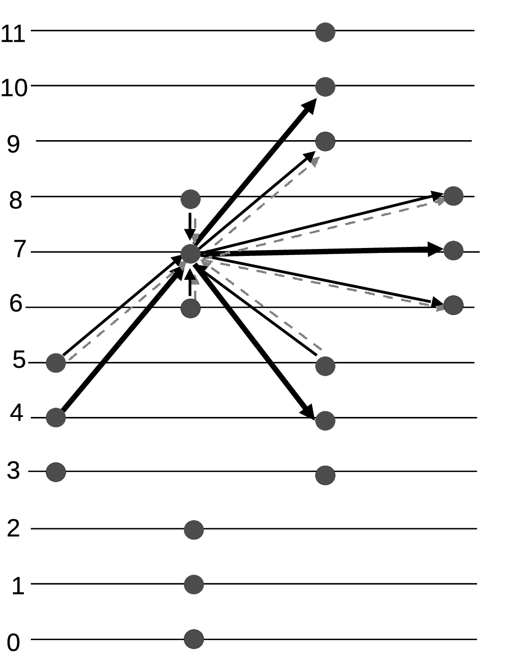
Consider an rectangle . It can be shown that it is tileable by -ribbons if and only if either or is divisible by . Assume without loss of generality that . An illustration of a 3-ribbon tiling for a rectangle is shown in Figure 8.
Let denote the subgraph of induced by vertices with , where and is the maximum possible level of a tile in an -ribbon tiling of . (For example, in Figures 8 and 8.)
Define growth factor
for , with the convention that , so that .
Let , the number of vertices at level , and , the number of vertices at levels between and , inclusive.
Lemma 3.
For all ,
Before proof, let us introduce some additional notation. If is an a.o. on a graph and is a subgraph of , then we write to denote the restriction of to . Obviously, is an a.o. on .
If and , then we call orientation on an extension of if and . Clearly, an extension is determined by and the orientations on edges in , where and denote the sets of edges of and , respectively. These orientations must be such that no directed cycle is created in . We denote the set of all extensions of from to as .
Proof of Lemma 3.
By restriction, every a.o. in corresponds to an a.o. in , . To prove the lemma, it is enough to show that for every there are no more than extensions of in .
Let
By abusing notation, we will also use , , to denote the subgraphs of induced by respective sets of vertices.
Now, if and , then
Moreover,
where is the set of edges between vertices in and vertices in . Since the orientations on are forced by partial orientation , the orientations assigned by extension of to edges in also completely determine the extension of . It follows that
In particular, in order to prove the lemma, it is enough to show that for every .
Next, note that and are complete graphs. (Indeed, the levels of any two vertices in differ by no more than , hence they are comparable with respect to the left-of relation, and therefore connected by an edge.) Also, note that the only edges with forced orientation in are the edges between vertices in .
On a complete graph, acyclic orientations are in one-to-one correspondence with linear orders on vertices. Now, an a.o. on determines a linear order on vertices of and the forced orientations on determine a linear order on vertices of . Then, the number of linear orders on consistent with given linear orders on and equals the number of ways to insert ordered vertices of between ordered vertices of . By an elementary combinatorial formula, this number equals
We showed that for every , and by observations above, this completes the proof of the lemma. ∎
Let and
| (1) |
In other words, is the highest level among those that have the most vertices. For example, in Figure 8, and .
Lemma 4.
If , then .
Here is the base of the natural logarithm.
Proof.
Proof of Theorem 2.4.
Let and be subgraphs of induced by vertices with and vertices with , respectively, where is as defined in (1). Then, it is clear that .
For , we can define the map . This is an injective map from to (since can be recovered unambiguously from and ), and therefore
Then, by using Lemma 4, we have
Similarly, by using the fact that graph is symmetric, we can obtain the estimate , and therefore,
Then,
Note that . Then, we have:
∎
3.6 Number of tilings of a generalized Aztec Diamond
Proof of Theorem 2.5.
It is easy to check that the Sheffield graph and the partial orientation of the generalized Aztec diamond for -ribbon tilings are isomorphic to the Sheffield graph and the partial orientation of for -ribbon tilings, that is, with that of domino tilings of the standard Aztec diamond. This implies that these graphs have the same number of acyclic orientations that agree with the partial orientation. Hence, the number of -ribbon tilings of equals the number of domino tilings of the standard Aztec diamond, and this number was computed in the celebrated result in [5]. ∎
Note that this proof provides a bijection between domino tilings of and -ribbon tilings of . In this bijection, two tilings correspond to each other if they induce the same acyclic orientation on the isomorphic Sheffield graphs of and . Intuitively, one can think about this bijection as that one can judiciously add squares to each domino tile of the domino tiling so as to lengthen the shape vertically and make it coincide with .
3.7 Exact value for the limit entropy of a stair region
The proof is based on the exact enumeration of the number of ribbon tilings for these regions.
Theorem 3.1.
The number of tilings of the stair region by -ribbons is given by the following formulas. If is odd, then
If is even, then equals the number of tiling of an rectangle by -tiles, namely


Proof.
Consider the case when is odd. Every tiling of the region by -ribbons has tiles, one tile in each level , , , . We denote these tiles . Then, the Sheffield graph that corresponds to this region has edges in the following list,
provided that both end-points are well defined. (See an example for in Figures 10 and 10).
Crucially, this graph does not have any edges with forced orientation, since (i) the differences between levels of tiles are even and therefore are different from , and (ii) every level has no more than one tile.
By Sheffield’s theorem, the number of tilings of the region is equal to the total number of acyclic orientations of the graph , since the partial orientation of is empty. If , then the graph is the complete graph and the number of acyclic orientations is .
If , then we use Stanley’s theorem ([16]) that the number of acyclic orientations of a graph equals to , where denotes the chromatic polynomial of the graph . The chromatic polynomial for the graph is calculated in Lemma 5, and we get the following formula for the number of acyclic orientations:
where . This proves the theorem for the odd .
For the case when is even, it is easy to check that the graph of the for -ribbon tilings coincide with the graph of for -ribbon tilings. This implies that the number of tilings is the same. ∎
Lemma 5.
Let be odd, let , and let graph be as defined in the proof of Theorem 3.1, with . Then, the chromatic polynomial of the graph is
| (2) |
Proof.
We use induction on and Read’s theorem from [12] that says that if a graph is a union of two subgraphs and , which overlap in a complete graph on nodes, then the chromatic polynomial of the graph is
| (3) |
where is the factorial monomial:
In our case the graph is the restriction of graph to vertices , , …, , and the graph is the restriction of graph to vertices , …, . They intersect in complete graph . (In the example in Figure 10, , and .)
The graph equals the complete graph on vertices with the edge removed. A well known property of chromatic polynomials relates the polynomial of a graph to the polynomials of the graphs obtained by a contraction and a removal of an edge, respectively. Namely, for every simple graph and for all ,
where denotes with the edge deleted, and denotes with the edge contracted to a point.
By applying this property to the complete graph , note that the removal of an edge leads to the graph and a contraction of leads to . Hence,
For the base of the induction, we note that if , then and the formula (2) is valid by what we just proved.
Appendix A Stanley’s results about the number of ribbon tilings


Stanley considers the ribbon tilings of connected skew shapes. (He uses the name border strip decompositions for these tilings, see an example in Figure 12.) A skew shape is the difference of two Young diagrams and , such that is inside of . In particular, skew shapes include all Young diagrams, and in particular, all rectangles. Stanley works under assumption that lengths of ribbons in such a tiling can be arbitrary, which is different from our assumption of fixed length.
In Exercise 7.66 (p. 470, with a solution on p. 521) in [17], it is shown that the number of ribbon tilings can be written as a product of certain Fibonacci numbers.
Here is a summary of Stanley’s result applied to an -by- rectangle with . The number of tilings of the rectangle is given by the product:
where are Fibonacci numbers, . (For example, for the rectangle and the square we have and , respectively.)
In particular, for squares, , we can write the entropy per unit area as
By using the asymptotic approximation for Fibonacci numbers, the asymptotic expression for the entropy per unit area is
where is the golden ratio. It is somewhat difficult to compare this result with our findings, since it not clear what is the average entropy per tile. The number of tiles is different in different Stanley’s tilings of an rectangle and we do not know how the expectation of in a random ribbon tiling depends on .
The second result was obtained in [18]. It is still assumed that the lengths of ribbons in a ribbon tiling are arbitrary. A ribbon tiling is called minimal if there is no other tiling with a smaller number of ribbons (see an example in Figure 12). For skew shapes, Stanley determined the number of tiles in a minimal tiling and the number of minimal ribbon tilings. If we specialize his results to -by- rectangles with , then the number of ribbons in a minimal tiling always equals . (So, for large rectangles, most of the tiles in a minimal tiling are long, with the average length equal .) In the case of rectangles with , Stanley’s formula for the number of minimal tilings reduces to
In particular, the per-tile entropy is
As a consequence, if is fixed and is growing then the asymptotic per-tile entropy does not depend on the average length of the tile . This is in contrast to our results, where the per-tile entropy grows at the logarithmic rate in the length of the tile.
If and both are growing, then the per-tile entropy grows at the logarithmic rate in the average length of the tile , similar to our results.
Acknowledgements
The second author was supported by Simons Foundation through the program “Mathematics and Physical Sciences–Travel Support for Mathematicians”, Award ID 523587.
References
- AGMSV [20] J. T. Akagi, C. F. Gaona, F. Mendoza, M. P. Saikia, and M. Villagra. Hard and easy instances of L-tromino tilings. Theoretical Computer Science, 815:197–212, 2020. URL https://doi.org/10.1016/j.tcs.2020.02.025.
- AL [19] P. Alexandersson and J. Linus. Enumeration fo border-strip decompositions and Weil-Petersson volumes. J. Integer Seq., 22(4), 2019. URL https://cs.uwaterloo.ca/journals/JIS/VOL22/Alexandersson/alex4.pdf.
- Chen [20] Y. Chen. Counting and sampling ribbon tilings of rectangles. PhD thesis, Binghamton University, 2020.
- CKP [01] H. Cohn, R. Kenyon, and J. Propp. A variational principle for domino tilings. J. Amer. Math. Soc., 14(2):297–346, 2001. URL https://doi.org/10.1090/S0894-0347-00-00355-6.
- EKLP [92] N. Elkies, G. Kuperberg, M. Larsen, and J. Propp. Alternating-sign matrices and domino tilings. I. J. Algebraic Combin., 1(2):111–132, 1992. URL https://doi.org/10.1023/A:1022420103267.
- HW [15] M. Hutchinson and M. Widom. Enumeration of octagonal tilings. Theoretical Computer Science, 598:40–50, 2015. URL https://doi.org/10.1016/j.tcs.2015.03.019.
- Kasteleyn [61] P. W. Kasteleyn. The statistics of dimers on a lattice. Physica, 27:1209–1225, 1961. URL https://doi.org/10.1016/0031-8914(61)90063-5.
- KMZ [96] R. Kaufmann, Y. Manin, and D. Zagier. Higher Weil-Petersson volumes of moduli spaces of stable -pointed curves. Comm. Math. Phys., 181:763–787, 1996. URL https://projecteuclid.org/journals/communications-in-mathematical-physics/volume-181/issue-3/Higher-Weil-Petersson-volumes-of-moduli-spaces-of-stable-n/cmp/1104287912.full.
- KP [04] M. Korn and I. Pak. Tilings of rectangles with T-tetrominoes. Theoretical Computer Science, 319:3 – 27, 2004. URL https://doi.org/10.1016/j.tcs.2004.02.023.
- Merino [08] C. Merino. On the number of tilings of the rectangular board with T-tetrominoes. Australasian Journal of Combinatorics, 41:107–114, 2008. URL https://ajc.maths.uq.edu.au/pdf/41/ajc_v41_p107.pdf.
- Pak [00] I. Pak. Ribbon tile invariants. Trans. Amer. Math. Soc., 352(12):5525–5561, 2000. URL https://doi.org/10.1090/S0002-9947-00-02666-0.
- Read [68] R. C. Read. An introduction to chromatic polynomials. J. Combinatorial Theory, 4:52 – 71, 1968. URL https://math.berkeley.edu/~mrklug/ReadChromatic.pdf.
- Richter [23] C. Richter. Covering rectangles by few monotonous polyominoes. Acta Mathematica Hungarica, 169:73–87, 2023. URL https://doi.org/10.1007/s10474-023-01308-8.
- Sheffield [02] S. Sheffield. Ribbon tilings and multidimensional height functions. Trans. Amer. Math. Soc., 354(12):4789–4813, 2002. URL https://doi.org/10.1090/S0002-9947-02-02981-1.
- [15] J. Spencer and L. Florescu. Asymptopia, volume 71 of Student Mathematical Library. American Mathematical Society, Providence, Rhode Island, 2014. URL http://dx.doi.org/10.1090/stml/071.
- Stanley [73] R. P. Stanley. Acyclic orientations of graphs. Discrete Mathematics, 5:171 – 178, 1973. URL https://doi.org/10.1016/0012-365X(73)90108-8.
- Stanley [99] R. P. Stanley. Enumerative Combinatorics, volume 2. Cambridge University Press, 1999. URL https://doi.org/10.1017/CBO9780511609589.
- Stanley [02] R. P. Stanley. The rank and minimal border strip decompositions of a skew partition. Journal of Combinatorial Theory, Series A, 100:349–375, 2002. URL https://doi.org/10.1006/jcta.2002.3307.
- TF [61] H. N. V. Temperley and M. E. Fisher. Dimer problem in statistical mechanics—an exact result. Philos. Mag. (8), 6:1061–1063, 1961. URL http://dx.doi.org/10.1080/14786436108243366.