Learning in a Single Domain for Non-Stationary Multi-Texture Synthesis
Abstract
This paper aims for a new generation task: non-stationary multi-texture synthesis, which unifies synthesizing multiple non-stationary textures in a single model. Most non-stationary textures have large scale variance and can hardly be synthesized through one model. To combat this, we propose a multi-scale generator to capture structural patterns of various scales and effectively synthesize textures with a minor cost. However, it is still hard to handle textures of different categories with different texture patterns. Therefore, we present a category-specific training strategy to focus on learning texture pattern of a specific domain. Interestingly, once trained, our model is able to produce multi-pattern generations with dynamic variations without the need to finetune the model for different styles. Moreover, an objective evaluation metric is designed for evaluating the quality of texture expansion and global structure consistency. To our knowledge, ours is the first scheme for this challenging task, including model, training, and evaluation. Experimental results demonstrate the proposed method achieves superior performance and time efficiency. The code will be available after the publication.
Index Terms:
non-stationary, multi-texture synthesis, generative adversarial networks (GANs), category-specific training, texture similarity.I Introduction
Texture synthesis, as one of the classical low-level computer vision tasks, has broad application prospects in image manipulation [1], image restoration [2], 3D reconstruction [3], and so on. Current texture synthesis methods can be roughly divided into single-texture synthesis (STS) and multi-texture synthesis (MTS). Fig. 1 (a) and (b) illustrate the difference. STS trains a model for each texture image separately. Though some methods perform well on either a single natural image [1, 4] or non-stationary texture image [5], they are all time-consuming since for each instance, they need to train a separate model for up to several hours. MTS methods are proposed to solve this and are trained on texture datasets by designing new training strategies [6] and network structures [7], or transforming the distribution of feature maps [8, 9]. Nevertheless, most MTS methods cannot deal with irregular and non-stationary textures, as shown in Fig. 1 (d). Moreover, global structures of the generated textures are severely distorted.


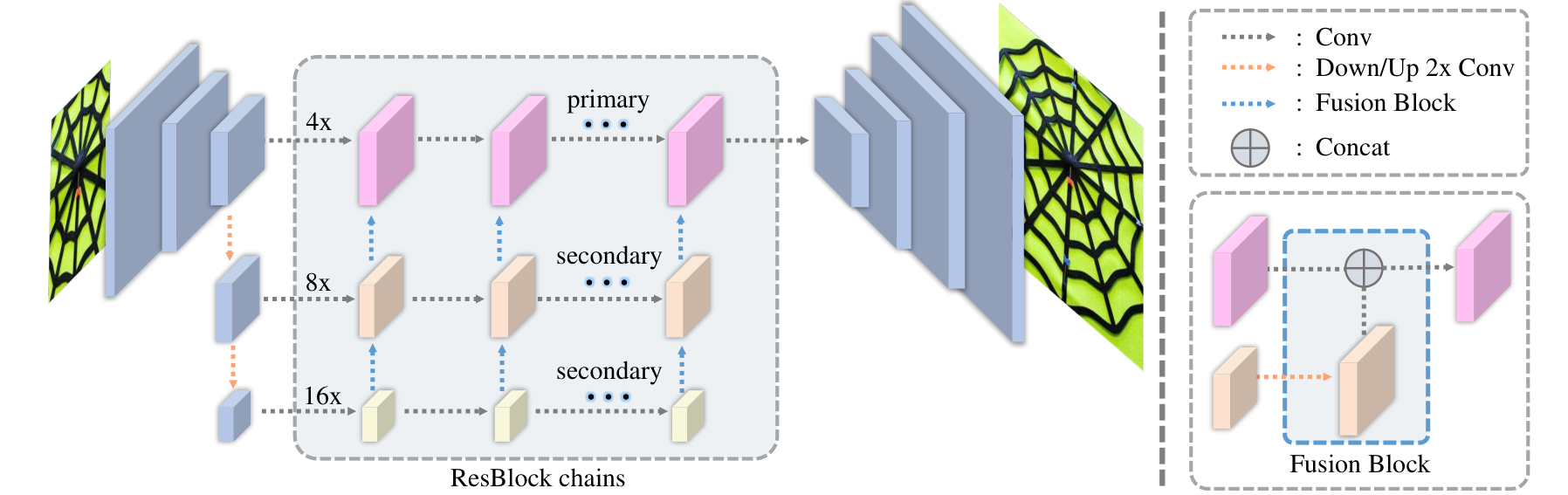
Based on the above observation, we focus on a challenging and meaningful task: non-stationary MTS in a single domain. That is, training a model to expand multiple different non-stationary textures of a single category while also preserving the global structure of the original textures. One noticeable benefit of this task is the well-trained models are able to produce multi-pattern variations of non-stationary textures that can not be observed in STS methods. Yet, one challenging aspect of this task is various scales of structures may appear in different samples or even in a single sample for non-stationary textures. In view of this, it is necessary to design a model with solid scale sensitivity to capture texture information of different scales. Therefore, we design a multi-scale generator by building multiple parallel network branches with different down-sampling rates, as shown in Fig. 2. The generator can preserve the global structure and generate meaningful and real-world texture images by training on multiple samples.
Besides, we observe that regularly, textures of the same category show similar structural patterns, e.g., cobweb textures usually show the same radial gradient expansion pattern. This hints to us that training on different samples in the same category benefits from the complementary information of each other. Otherwise, if training the model on samples from different categories, it is likely to have much longer training time and greater learning difficulty. Therefore, we propose a simple and effective training strategy, that is, category-specific training rather than random training on different categories. We prove that the model can learn the structures and expansion patterns of a specific texture category reasonably well under this scheme. More importantly, once a model is trained on a class of textures, it can be extended to arbitrary unseen images of the same category by a fast fine-tune phase since the pre-trained model is already knowledgeable about basic strategies to expand the inputs. We can also use a continual learning-based training method so that the final model can handle several categories at the same time.
In search of metrics for evaluating non-stationary multi-texture synthesis methods, we found regularly used metrics are not suitable to fully demonstrate the actual performance of different methods. To mitigate this problem, we contribute a metric named Multi-Scale Texture Similarity (MSTS). It is calculated upon the distribution distance between multi-scale deep features extracted from a pre-trained texture recognition model. In this way, it can not only evaluate whether the generated images preserve the global structure, but also evaluate the quality of texture synthesis. This is a multi-scale metric that considers the overall global structure and meanwhile focuses on local texture details. Its effectiveness is verified through our user study.
In summary, the contributions can be listed as follows:
- 1.
We systematically introduce a new generative task: non-stationary multi-texture synthesis in a single domain, including manifesting several applications and potential difficulties of this task.
- 2.
We propose an effective scheme for this task, which includes a multi-scale generator, a category-specific training strategy, and a texture similarity metric. Quantitative and qualitative results show the superiority of our method in image quality and time efficiency.
II Related work
Conventional approaches of example-based texture synthesis have achieved fine results on stationary textures. Image melding [10] presents a patch-based optimization method for synthesizing a gradual transition region between two images. Self-tuning [11] was proposed as a non-parametric texture optimization algorithm via weighted guidance channels. Recently, deep learning methods have emerged because of their excellent ability to extract meaningful high-level and low-level features. We mainly introduce these from two aspects:
Single-Texture Synthesis. Gatys et al. [12] propose a seminal optimization-based method for this task using CNN. They optimize the input by matching the Gram matrices extracted by VGG network [13] between the generated image and the reference image. Liu et al. [14] improve the CNN-based training method by incorporating the Fourier spectrum constraints, making the output images preserve large quasi-periodic structures. Rodriguez et al. [15] generate regular repeatable textures by finding the minimal repeating pattern in single images. Spatial generative adversarial network (SGAN) [16] is the first GAN [17]-based texture synthesis method, treating input noise as a whole spatial tensor. To handle non-stationary textures, Zhou et al. [5] present another GAN-based model for texture expansion via self-supervised training. Their method is effective for challenging textures with large-scale global structures. InGAN [18] improves this method by inserting a geometric transformation layer into the generator, enabling the model to produce outputs of different sizes and shapes. TileGAN [19] combines smaller resolution outputs of GANs to form a large-scale non-homogeneous texture. Recently, SinGAN [1] proposes multi-stage generators trained on a single natural image, learning the internal distribution of patches within an image. Some follow-up works, such as ConSinGAN [4], SinIR [20], PetsGAN [21] are devoted to speed up the learning efficiency of SinGAN [1]. They can do well for images with independent objects but fail for global non-stationary structures such as those in Fig. 7. Besides, Darzi et al. [22] capture local texture properties by computing a co-occurrence tensor. Zhou et al. [23] compute the Guided Correspondence Distance to improve the CNNMRF model for high-quality texture optimization. However, it should be noted that all single-texture models are time-consuming and costly. Therefore, some works studied how to process multiple textures within one model. Our work is exactly to cope with multi-texture synthesis.
Multi-Texture Synthesis. Bergmann et al. extend their SGAN [16] as PSGAN [24], allowing the model to process multiple periodic textures concurrently. Meanwhile, Li et al. [6] introduce an incremental learning strategy so as to deal with multiple textures within one model. Other efforts performed MTS by adaptively editing intermediate feature maps of the encoder. WCT [8] is a typical method of universal texture synthesis through whitening and coloring operations on features, but the generated images destroy the global structures of input textures according to Fig. 8. Transposer [25] treats the encoded feature map as transposed convolution filters and the self-similarity map as the corresponding input. Mardani et al. [26] view texture synthesis as local Fast Fourier Transform upsampling and performed FFT in feature space for universal texture synthesis. Texture mixer [9] is trained on datasets, but its three latent-space operations destroy the global structure. In addition, Shi et al. [7] propose a pseudo optimizer to unfold the iterative optimization procedure of DeepTexture [12] into a feed-forward neural network, realizing fast texture synthesis. However, these approaches cannot handle non-stationary textures according to our observation in Fig. 8 and the statement in their paper. In view of the problems, we present a multi-branch generator for MTS to cope with non-stationary textures effectively.
Image Quality Assessment. It remains a problem that how to evaluate the effect of texture expansion and whether the global structure is preserved in the process of texture synthesis. The mainstream full-reference image quality assessment (IQA) models [27] can be roughly divided into pixel-level methods [28], structural similarity methods [29, 30] and deep-feature based methods [31, 32, 33]. MSE [28] calculates the distance among pixel pairs and SSIM [29] separates image structure from brightness and contrast, but sometimes they are inconsistent with the subjective evaluation. Deep-feature based methods, eg. FID [31] and DISTS [32] extract image features via a pre-trained classification network and then define some operations on them to capture the semantic and structural information. In addition, Wu et al. [34] propose the global and local textureness assessments to automatically guide better texture exemplar extraction for texture synthesis input. However, as shown in Fig. 5, none of these methods are competent for non-stationary multi-texture expansion tasks.
III Method
III-A Multi-Scale Model for Multi-Texture Synthesis
Non-stationary textures exhibit various scales of patterns, either among different samples of the same category or in a single sample, such as the peacock feather in Fig. 1 (d). It is challenging for single-scale generators [5, 18] to cope with multiple non-stationary textures. In light of this, we propose to build a generator with the capability to capture multiple scales of structure statistics for non-stationary multi-texture synthesis. This is a unique consideration to previous works, partially because they haven’t considered the scenario of non-stationary MTS.
Our final model, wrapping up this kind of generator, is named as Multi-Texture GAN (MTGAN). As shown in Fig. 2, it consists of multiple branches (one primary branch and several secondary branches) with different receptive fields. The primary branch is responsible for image encoding and decoding, while the secondary branches are to provide multi-scale information to the primary branch. Firstly, each branch processes information of different scales via different down-sampling rates. Then, feature maps of different scales are fed into the corresponding residual block [35] chains, where each chain consists of six identical residual blocks.
A critical step is how to fuse the information of different branches in an effective way. Initially, we try to fuse at the end of the residual block chains. The results are close to the model with only one branch, indicating that the primary branch does not obtain much valid information from secondary branches, as Fig. 12 shown. To fill up the information gap, we develop a feature fusion strategy to fuse the output of each residual block of different branches in a bottom-up manner. Such fusion can be formulated as
| (1) |
where is the feature map of small scale and is that of the adjacent large scale branch. concatenates with after upsampling, followed by a convolution to adjust the number of feature channels. With the branch-wise and layer-wise fusion strategy, these branches work collaboratively to make the model sensitive to both local details and global structure. At last, the decoder with an extra upsampling operation transforms the fused feature into an expanded texture image. More details about the architecture can refer to Sec. IV-A.
Multi-scale mechanism is a general consideration across many vision tasks. In this work, we consider several options that can be adapted for the non-stationary MTS task. Some typical examples of multi-scale design for other tasks endorse new network architecture design such as HRNet [36], insert a multi-scale context module like ASPP [37], etc. However, we believe our multi-scale generator is more beneficial to the task. Specifically, each fusion block in MTGAN fuses features of two scales (branch-wise), while HRNet [36] directly fuses features from multiple scales ( scales) via upsampling in different stages. The upsampling rate may reach up to 8 times, thereby induces much noise and yields apparent artifacts in the results. ASPP [37] also performs worse than our method supported by experiments. We hypothesize the common practice of applying such context modules only before the output layer is unable to capture texture scale variance. In contrast, our feature fusion is applied for all ResBlocks (layer-wise) to create enough flexibility for modeling scale variance of non-stationary textures. The comparison with these methods in the experiment shows the effectiveness of MTGAN.
III-B Category-Specific Training
We use three basic loss functions, including adversarial loss [17] , style loss [12] , and perceptual loss [38] , as the optimization objectives of our model. All these loss functions are defined between target images and generated images. We use adversarial loss to ensure the fidelity of the generated images. The style loss and the perceptual loss are computed upon the representations obtained from a pre-trained VGG [13] model to secure training stability in early stages. The full objective is defined as:
| (2) |
where and are the generator and the discriminator.
The existing multi-texture synthesis methods [6, 25] randomly select several texture images and then feed them into the neural network for training. However, due to the great difference in the global structure and spatial scale of non-stationary textures from different classes, it is difficult to train a single powerful model that can perform well on all textures. To reduce learning difficulty and improve synthesis quality, we propose a category-specific training strategy. More concretely, only one category of textures is used to train the network during the training phase. In this way, the model can easily grasp the texture structure and features of a specific category by making full use of the complementary information among samples. Moreover, once a model on a specific category is trained, we propose two training strategies to easily extend this model to other instances of the same category or even textures of a different category.
Extension at the instance level from the same category. Such extension is implemented by a fast fine-tune phase. Specifically, we load the trained model for a category and then input one unseen image of the same class as training data, fine-tuning for several iterations. To avoid catastrophic forgetting, we sample the old data of this category at a frequency of 20 during the phase. Given this replay-based strategy, not only can our model handle the unseen image, but it can still handle previous samples. Empirically, we found 900 iterations with batch size 4 are enough to make the fine-tuned model support a good expansion of such an unseen image. As shown in Tab. III, our model significantly reduces the time cost on unseen textures compared to STS models.
Extension at the category level. After we have trained MTGAN on one category of texture images, our approach also allows this trained model to further handle more categories jointly. To be more practical and flexible for real application scenarios, the data of old classes are not available but our strategy can still avoid catastrophic forgetting of the old classes when coping with new classes. Inspired by LwF [39] and LwF-GR [40], we apply a continual learning strategy to achieve this target. Specifically, we first train a model on a category to a near-optimal state (8000 epochs). Then, we add a new decoder to the generator to deal with the coming new category. Note that when the model is trained for the new data, the previous data is not available, thus, we apply a distillation loss to the old decoder to prevent forgetting. is generated by when the new model is initialized with old parameters before training, and is the output from during training. is similar as besides the term and the regularization term:
| (3) |
We compute through the old pre-trained discriminator without optimizing the old discriminator since the old discriminator is already knowledgeable to identify generations of the old category. and are the outputs by feeding and to the old discriminator. To deal with the new domain, we let . The detailed algorithm of this strategy is depicted in Algorithm 1. The continual learning strategy to extend the model to new categories can cater to the emergent open-world scenario [41].
III-C Multi-Scale Texture Similarity
According to the user study in Fig. 5, we find currently available metrics for evaluating non-stationary texture expansion performance are not in line with human evaluation. This motivates us to design a more suitable metric for non-stationary expansion evaluation. Our metric named Multi-Scale Texture Similarity (MSTS) is inspired by FID [31] to calculate the distance of distributions between two sets of deep features. The first difference is we obtain deep features of the input texture images from a DTD [42]-pretrained DEP model [43] instead of an ImageNet [44]-pretrained Inception [45] model. Texture images are not object-centric as ImageNet images, thus the DTD-pretrained model is more related to our task.
Another major difference is FID calculates the distance of distributions between two sets of images while MSTS calculates the similarity between the internal distributions of patches within the original image and the generated image. Given the internal distributions of the original texture and the generated texture as and , respectively. The equality holds iff. where is arithmetic operations of input data . Here we replace with the 128-dimensional feature vector output from the penultimate layer of the DEP model. We assume the feature to follow a multidimensional Gaussian, and we utilize Wasserstein-2 distance to measure the similarity between these two distributions. Our final metric is thus given by
| (4) |
where and are the mean and covariance of . Analogously, and are the mean and covariance of .
Furthermore, multi-scale statistics are helpful for capturing structure and scale variance [29]. To this end, MSTS is designed with a multi-scale mechanism, which is also hugely different from FID. In addition to calculating scores on the full image, we also randomly crop patches of different scales with 16 samples for each scale, where the scales are set to , , of the original image. Finally, we have four scores , , , corresponding to four different scales ranging from large to small. MSTS score can be expressed as a combination of the four scores:
| (5) |
Note we multiply MSTS by to enlarge the final value to make it more intuitive. Such a metric can jointly evaluate global texture structure and local texture details as verified through our user study.
IV Experiments
IV-A Datasets and Implementation Details
Our experiments are conducted on Describable Texture Dataset (DTD) [42], which consists of 47 texture categories with 120 images in each class. This dataset contains a large number of non-stationary texture images with complex backgrounds and various scales. Considering the feasibility of the experiments for evaluating non-stationary multi-texture synthesis performance, we form a subset by choosing 11 representative and challenging non-stationary classes: braided, bubbly, bumpy, cobwebbed, cracked, fibrous, honeycombed, scaly, spiralled, stained, veined. We denote this selected dataset as DTD-11. Fig. 3 shows the results of our approach on DTD-11 dataset. The proposed method can cope with various challenging non-stationary textures. Besides, we also collected some challenging texture images from the Internet to test the generalization ability of our method on unseen images.
The detailed generator architecture of MTGAN is shown in Fig. 4. We adopt the 6-layers PatchGAN [46] discriminator to alternatively train with the generator. We train our model using Adam [47] optimizer, where its hyper-parameters are set as , and . We train each category of textures individually for 8000 epochs with batch size 4 on one NVIDIA Titan Xp. The learning rate keeps unchanged for the first 4000 epochs and then linearly decays to zero over the remaining 4000 epochs.

IV-B Evaluation of MSTS
We evaluate the effectiveness of MSTS for texture synthesis tasks via a user study. We first collect 5 images of each category generated by each of the following models: self-tuning [11], Non-stat. [5], InGAN [18], SinGAN [1], ConSinGAN [4], and our model. We then create a questionnaire with 55 questions, where each question asks how well the generated image is expanded according to the original structure and texture arrangement. Then, we distribute the questionnaire to twenty users to sort the images of each question from 1 (least pleasant) to 6 (most satisfactory). Tab. I (Pref.) shows the average preference scores for the user study. Besides, we also evaluate the performance of these models on several objective metrics: SSIM [29], FID [31], DISTS [32] and MSTS. To verify the effectiveness of MSTS, we rank all the models according to each metric, as shown in Fig. 5. The sorting result of MSTS is more consistent with our user study, which demonstrates MSTS is comparatively more suitable for evaluating non-stationary expansion results.

In addition, we test the sensitivity of MSTS and other three metrics when encountering textures with structure or texture distortions. To test global structure sensitivity, we apply two distortion operations: shuffling texture patches and image warping. We also apply two other distortions to test texture change sensitivity: Gaussian blurring and randomly removing pixels. As shown in Fig. 6 (a) & (b), when the distortion is weak (disturbance level [31] is 1), MSTS value is competitive to other metrics. When the structure distortion becomes more severe, MSTS makes the highest responses. Also, note that the curve slopes of other metrics after disturbance level 1 are quite smaller than that of MSTS. These two plots unveil that MSTS is more sensitive to large structure distortion than other metrics. Moreover, MSTS presents more reasonable responses to texture distortions, as show in Fig. 6 (c) & (d). When the disturbance level is 1, the subjective visual difference of the images is subtle, resulting in a smaller value of MSTS. By increasing the disturbance level, the image quality decreases significantly, and MSTS shows the most sensitive responses. Consequently, MSTS can be a more suitable and effective metric for the texture synthesis task.
Since MSTS estimates the internal patch distribution within a single image, 16 patch samples for each spatial scale can already obtain stable results. We conduct MSTS evaluation of “Ours (Multi)” in Tab. I w.r.t. different sample sizes with 50 random seeds for each sample size. Then we calculate the mean and standard deviation for each sample size over 50 seeds (size@mean/std): 8@99.46/4.50, 16@98.34/2.13, 32@98.28/1.80, 64@98.51/1.17. Actually, the results reported in the paper are the mean values over 50 random seeds. We can obtain more stable results by increasing the sample size but the evaluation time will increase.
IV-C Evaluation of MTGAN

| Methods | MSTS | SSIM | DISTS | FID | Hist. | Pref. |
|---|---|---|---|---|---|---|
| Self-tuning | 109.43 | 0.0539 | 0.3653 | 288.7 | 0.975 | 2.20 |
| Non-stat. | 107.99 | 0.0725 | 0.3156 | 209.6 | 0.827 | 2.85 |
| InGAN | 103.48 | 0.1818 | 0.3074 | 222.3 | 0.667 | 2.91 |
| SinGAN | 126.83 | 0.0664 | 0.3465 | 259.1 | 0.844 | 2.08 |
| ConSinGAN | 205.14 | 0.0561 | 0.3649 | 337.2 | 0.860 | 1.91 |
| Ours (Multi) | 98.34 | 0.0831 | 0.3141 | 233.4 | 0.838 | 3.55 |
| Ours (Single) | 97.68 | 0.0845 | 0.3061 | 196.9 | 0.862 | - |
We compare our MTGAN with STS and MTS methods qualitatively and quantitatively. We use MSTS, SSIM, DISTS, and FID to evaluate the quality of the synthesized textures comprehensively. Besides, we also compare the time efficiency of these methods in the training and inference phases. These comparisons show the superiority and practicability of our method on non-stationary texture synthesis.
Compare with single-texture synthesis methods. Since STS methods can usually deal with non-stationary textures and generate better results than MTS methods, we compare MTGAN with them to demonstrate our high generation quality and superior time efficiency. We follow the evaluation protocol of [25], also an MTS method to compare with STS methods. Besides the metrics mentioned above, we utilize color histogram comparison and user study to comprehensively assess these methods. The recent related competitors for STS are self-tuning [11], Non-stat. [5], InGAN [18], SinGAN [1] and ConSinGAN [4]. We follow the implementation of these methods in their papers. Considering the fact that STS models are too slow to be trained on all images of DTD-11, we randomly select 55 samples uniformly from 11 categories to evaluate. To compare with them, we train our model under two settings: 1) Multi: model trained on all the data of each category in DTD-11 separately. We then select the 55 corresponding images from the synthesis results for comparison. Note, our model is not fine-tuned for these images. 2) Single: model trained on a specific image for 10000 iterations by completely analogy to the training strategy of other STS models.
For inference, we randomly crop a patch for each image and feed it into these models to generate outputs with a size of . As Fig. 7 shows, our model performs well in various non-stationary textures with different scales and categories. While preserving the global structure of the input textures, our results exhibit fewer artifacts. Self-tuning cannot follow the global structure, and its results tend to be highly repetitive. SinGAN and ConSinGAN are incompetent for textures with large-scale structure, and their results retain only basic lines and color information. InGAN maintains the global structure, but it suffers from obvious color deviation, for instance, the first row of InGAN is darker than the input and the second row is brighter. Non-stat. achieves balanced results, but some show unreasonable patterns. For example, the cobwebbed images in the first and third rows present two centers while it is known that cobweb generally has only one center, and there are many damaged honeycombed parts in the lower right corner of the fourth row. Together, the results establish the superiority of our multi-scale design for MTGAN because the model can maintain the layouts and color distribution of original textures, at the same time, performing natural expansion.
We quantitatively evaluate all the methods on these 55 images, and show the average scores in Tab. I. Our method achieves SOTA performance. SSIM is computed by resizing the generated images to their input sizes. As a result, it has small reference value since a result that is simply the super-resolution of the input would obtain the highest score. Compared with MTGAN (Multi), though InGAN performs better in DISTS, FID, it presents severe color distortion problem as hinted by the Hist. in Tab. I and thus performs worse than our method in the user study. The phenomenon is also observed in Fig. 7. Besides, our approach achieves significantly better time efficiency than the STS models when training and extending to unseen images, as shown in Tab. III.

| Methods | MSTS | SSIM | DISTS | FID |
|---|---|---|---|---|
| PO | 345.13 | 0.0431 | 0.3610 | 181.58 |
| Texture Mixer | 319.28 | 0.0494 | 0.4448 | 231.18 |
| WCT | 223.39 | 0.0748 | 0.3869 | 219.18 |
| Neural FFTs | 206.83 | 0.0692 | 0.3758 | 164.84 |
| Our method | 156.66 | 0.0911 | 0.3323 | 128.93 |
| Methods | Training | Inference | Unseen img. |
|---|---|---|---|
| Self-tuning | - | 4.5 mins | 4.5 mins |
| Non-stat. | 5.0 hrs | 51.6 ms | 5.0 hrs |
| InGAN | 4.1 hrs | 430 ms | 4.1 hrs |
| SinGAN | 2.5 hrs | 379 ms | 2.5 hrs |
| ConSinGAN | 0.9 hrs | 200 ms | 0.9 hrs |
| PO | 0.42 hrs | 92 ms | 92 ms |
| Texture Mixer | 1.25 hrs | 850 ms | - |
| WCT | - | 8 s | 8 s |
| Neural FFTs | 0.97 hrs | 210 ms | 210 ms |
| Our method | 0.18 hrs | 60 ms | 5 mins |
Compare with multi-texture synthesis methods. MTS methods can handle multiple samples within one model. To demonstrate the powerful ability of our MTGAN to cope with non-stationary textures, we compare MTGAN with some recent and typical MTS methods such as WCT [8], Texture Mixer [9], PO [7], and Neural FFTs [26]11 1 Since the official code of Neural FFTs [26] is not available, we reproduced its model by ourselves and report the results.. For a fair comparison, all the models are optimized through the proposed category-specific training strategy. Other settings of training details follow their original papers. PO cannot be applied to texture expansion and its outputs are resized to the sizes of inputs.
Tab. II indicates that our MTGAN outperforms other MTS methods under all metrics. The qualitative comparisons in Fig. 8 show that all the other methods cannot deal with non-stationary textures, without preserving the global structure or just enlarging the input images. Texture Mixer mainly retains the color information and few texture details of the input texture. The structure is seriously destroyed, and only stationary textures can be generated. Though better than Texture Mixer, WCT shares the same problem. According to the observation in Fig. 8 and the statement in the original paper [26], Neural FFTs cannot expand non-stationary textures and produces many artifacts. In contrast, our method synthesizes natural expansions without destroying global structures and producing artifacts. Also, the time efficiency of our method achieves state-of-the-art performance compared to other MTS methods.
Time efficiency comparisons. We count the training and inference time of all the STS and MTS models in Tab. III. For STS models, we evaluate the training time on a single image. For MTS models, we get the training time on a category of textures (120 images) and then compute the average time on one image. The inference time is calculated by generating an image of size . All the evaluations are conducted on one NVIDIA Titan Xp with an Intel Xeon CPU E5-2637 @ 3.50GHz. Compared with STS methods, MTGAN reduces the training time of each texture by 5-27 times. Meanwhile, our inference time is competitive to that of Non-stat. and outperforms others, indicating that our multi-scale design does not harm inference speed. Compared to MTS methods, MTGAN shows obvious superiority both in training and inference time, which reveals that it is better and more applicable to real-world scenarios.
IV-D Evaluation of training strategies

This part is to show the effectiveness of the category-specific training strategy, the fast fine-tune strategy for instances in the single category, and the continual learning strategy to extend a trained model to a different domain.
Effectiveness of the category-specific training strategy. One straightforward strategy to optimize our model is random training, where we randomly select 110 images from the whole DTD-11 and mix them together to train MTGAN; For category-specific training, the 110 training images are from the same category. Fig. 9 shows several results of different training strategies. Compared with random training, category-specific training achieves apparently better results.
Extension at the instance level from the same category. In order to verify the fast expansion strategy at the instance level, we experiment with Internet images for each texture category. We fine-tune a pre-trained model with an unseen image for 900 iterations and compare to a model that is trained from scratch for 900 iterations. As shown in Fig. 10, training from scratch can hardly capture sufficient texture information and generate reasonable images.
Besides, we conduct another experiment to verify the stability and generalization of our model. We sequentially fine-tune a well-trained model on three unseen honeycombed textures. That is, when we fine-tune the model on the second texture, the first image is added to the old sample set. Fig. 11 shows the sequential fine-tuning results of these three textures. It can be seen that although the model has been fine-tuned three times sequentially, it can still cope with old samples well.
In general, STS models usually takes at least two hours to generate a new reasonable result (Tab. III), our strategy is efficient by reducing the time to 5 minutes. Although some MTS methods take less time than ours to expand unseen images, they cannot cope with non-stationary textures. Therefore, this strategy facilitates the stability and generalization of our model, and dramatically reduces the time cost on unseen textures compared to STS models.
Extension at the category level. Our method can cope with multiple categories jointly within one model through a continual learning-based training strategy. The fourth row of Fig. 9 presents the results of different categories from one model under the continual learning strategy. We specify 8,000 epochs for each category, and we successively train five categories considering the time and computational cost. The results obtained by continual learning are noticeably better than random training, though with a slight decrease compared to the category-specific training strategy.


IV-E Ablation Study

We evaluate several design choices of our generator. Fig. 12 and Tab. IV demonstrate the qualitative and quantitative comparison results. Note that adding a new branch is essentially introducing a new scale because the down-sampling rate of each branch is different. From Fig. 12, the third row (“One Scale”) shows that a single-scale network cannot naturally expand large-scale textures, but simply enlarge them. We observed a similar problem in training STS methods on a category level. Specifically, the “One-Scale” setting of our MTGAN is equivalent to the architecture of Non-stat. [5]. In other words, when training Non-stat. with multiple textures following our category-specific training strategies, Non-Stat. presents the same phenomena as shown in the third row of Fig. 12. When adding another branch, the “Two Scales” model can conduct preliminary texture expansion with more scale variance. However, the size of hexagons is different, and the color and structure are inconsistent with the original image. Furthermore, when adding the third branch (“Ours”), more satisfactory results can be obtained since enough multi-scale information is gathered to deal with such a structure. On the other hand, it is even better for the multi-scale model to handle textures with different structure scales in a single image. For the third column of Fig. 12, the original image consists of a small-scale cobwebbed texture and a middle-scale railing texture. It is difficult to handle these two textures jointly in a single-scale model, but it can be done in a multi-scale model. Besides, adding more scales (“Four Scales”) will not improve the overall performance yet cause the increase of model capacity, according to our experiment of adding four scales (32 down-sampling). The feature maps of the branch with the highest down-sampling rate are quite small (), introducing more artifacts during the fusion phase. Therefore, to balance the performance and efficiency, we choose three scales as default.
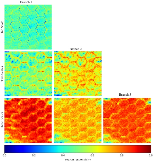
To further intuitively verify the effectiveness of our multi-scale design, we visualize the feature map output by the last ResBlock of each branch. Taking the second column of Fig. 12 as an example, the visualization results are shown in Fig. 13. When the generator has only one branch (“One scale”), the visualization reflects some focus on local details such as edge information yet shows a rather faint response to global structure. After adding a branch (“Two scales”), “Branch 2” pays more attention to the shape information of internal texture elements, such as the shape of a hexagon. “Branch 2” integrates this information into the primary branch (“Branch 1”) so that “Branch 1” shows more sensitivity to local details and can also capture some shape information. Moreover, after adding the third branch (“Three Scales”), “Branch 3” and “Branch 2” relatively concentrate on the global structure and spatial arrangement of textures. The primary branch can capture both local details and global structure. With the assistance of our fusion strategy, these three branches work collaboratively to make the model sensitive to both local details and global structure, making non-stationary texture expansion more feasible.
| Methods | MSTS | SSIM | DISTS | FID |
|---|---|---|---|---|
| End Fusion | 235.41 | 0.0602 | 0.3150 | 125.69 |
| One Scale | 241.48 | 0.0616 | 0.3144 | 139.48 |
| Two Scales | 230.48 | 0.0619 | 0.3124 | 129.70 |
| Four Scales | 220.72 | 0.0589 | 0.3139 | 126.68 |
| ASPP | 234.96 | 0.0597 | 0.3102 | 137.39 |
| HRNet | 338.60 | 0.0295 | 0.3781 | 181.95 |
| Ours (Three Scales) | 216.28 | 0.0621 | 0.3046 | 123.33 |
Feature fusion of different branches can be conducted at the end of the residual block chains rather than in every internal residual block. However, we find the result of such fusion manner (“End Fusion”) is almost the same as that of a single-scale model, which implies that the primary branch does not obtain much valid information from secondary branches. This proves the effectiveness of our fusion strategy for our task.
We also compare some representative multi-scale designs by applying ASPP [37] module to the one-scale MTGAN and replacing the multi-branch architecture of MTGAN with HRNet [36]. As shown in Fig. 12 and Tab. IV, both models are inferior to the multi-scale MTGAN for non-stationary multi-texture synthesis. Specifically, HRNet suffers from artifacts and color distortion, and ASPP cannot deal with large-scale textures well. We hypothesize the performance gap is due to what we described in Sec. III-A.


V Applications
High-Resolution Texture Synthesis. We can obtain textures of different resolutions by repeating the expansion until generating a high-resolution image. That is, we feed the output of the model as its input circularly. In this way, the proposed method synthesizes a result for each texture, as shown in Fig. 14. Then, we can crop the large-scale texture to our desired sizes/aspect-ratios to produce wallpapers. Such wallpapers have visual coherence, unlike those rigidly spliced by multiple identical patches with obvious seams in daily life. The details and structure of the texture can be well preserved.
Multi-Pattern Output. Training a single model with a class of texture images can potentially empower the model to yield diverse generations. In order to manifest this intriguing property, we feed an image to a trained model and obtain diverse outputs by adding noise or performing some random data augmentations (brightness, contrast, saturation, hue) to the input image. We observe the model can output multiple variations of the same texture category while STS models lack this ability. These results in Fig. 15 indicate that our category-specific training strategy brings rich non-stationary texture patterns to the model, and thus can carry out texture-guided multi-pattern image style transfer and WordArt design.
VI Conclusions
We focus on non-stationary multi-texture synthesis by designing a systematic scheme including model, training, and evaluation. Extensive experiments demonstrate the effectiveness and superiority of our approach. Moreover, our model can produce multi-pattern generations of the same category compared to other texture synthesis models.
The introduced task offers a meaningful research direction to the community. It pushes texture synthesis to practicality, generating more difficult and non-stationary texture images with high fidelity and low time cost. From the application standpoint, these rapidly synthesized non-stationary textures can provide more exquisite and plentiful raw materials for fashion designers, artists, and computer game developers. Academically, the proposed multi-scale architecture may be used for more image-to-image translation tasks, and the category-specific training strategy may offer insight to other class-incremental learning algorithms. We wish the proposed Multi-Scale Texture Similarity could be a general metric to evaluate the texture property in the computer vision community.
References
- [1] T. R. Shaham, T. Dekel, and T. Michaeli, “Singan: Learning a generative model from a single natural image,” in Proc. ICCV, 2019, pp. 4570–4580.
- [2] M. Bertalmio, L. Vese, G. Sapiro, and S. Osher, “Simultaneous structure and texture image inpainting,” IEEE Trans. Image Process., vol. 12, no. 8, pp. 882–889, 2003.
- [3] X. Zeng, Z. Wu, X. Peng, and Y. Qiao, “Joint 3d facial shape reconstruction and texture completion from a single image,” Computational Visual Media, vol. 8, pp. 239–256, 2022.
- [4] T. Hinz, M. Fisher, O. Wang, and S. Wermter, “Improved techniques for training single-image gans,” in Proc. WACV, 2021, pp. 1300–1309.
- [5] Y. Zhou, Z. Zhu, X. Bai, D. Lischinski, D. Cohen-Or, and H. Huang, “Non-stationary texture synthesis by adversarial expansion,” ACM Trans. Graph., vol. 37, no. 4, p. 49, 2018.
- [6] Y. Li, C. Fang, J. Yang, Z. Wang, X. Lu, and M.-H. Yang, “Diversified texture synthesis with feed-forward networks,” in Proc. CVPR, 2017, pp. 3920–3928.
- [7] W. Shi and Y. Qiao, “Fast texture synthesis via pseudo optimizer,” in Proc. CVPR, 2020, pp. 5498–5507.
- [8] Y. Li, C. Fang, J. Yang, Z. Wang, X. Lu, and M.-H. Yang, “Universal style transfer via feature transforms,” in Proc. NeurIPS, 2017, pp. 386–396.
- [9] N. Yu, C. Barnes, E. Shechtman, S. Amirghodsi, and M. Lukac, “Texture mixer: A network for controllable synthesis and interpolation of texture,” in Proc. CVPR, 2019, pp. 12 164–12 173.
- [10] S. Darabi, E. Shechtman, C. Barnes, D. B. Goldman, and P. Sen, “Image melding: Combining inconsistent images using patch-based synthesis,” ACM Trans. Graph., vol. 31, no. 4, pp. 1–10, 2012.
- [11] A. Kaspar, B. Neubert, D. Lischinski, M. Pauly, and J. Kopf, “Self tuning texture optimization,” in Comput. Graph. Forum, vol. 34, no. 2. Wiley Online Library, 2015, pp. 349–359.
- [12] L. Gatys, A. S. Ecker, and M. Bethge, “Texture synthesis using convolutional neural networks,” in Proc. NeurIPS, 2015, pp. 262–270.
- [13] K. Simonyan and A. Zisserman, “Very deep convolutional networks for large-scale image recognition,” arXiv preprint arXiv:1409.1556, 2014.
- [14] G. Liu, Y. Gousseau, and G.-S. Xia, “Texture synthesis through convolutional neural networks and spectrum constraints,” in Proc. ICPR. IEEE, 2016, pp. 3234–3239.
- [15] C. Rodriguez-Pardo, S. Suja, D. Pascual, J. Lopez-Moreno, and E. Garces, “Automatic extraction and synthesis of regular repeatable patterns,” Comput Graph, vol. 83, pp. 33–41, 2019.
- [16] N. Jetchev, U. Bergmann, and R. Vollgraf, “Texture synthesis with spatial generative adversarial networks,” arXiv preprint arXiv:1611.08207, 2016.
- [17] I. Goodfellow, J. Pouget-Abadie, M. Mirza, B. Xu, D. Warde-Farley, S. Ozair, A. Courville, and Y. Bengio, “Generative adversarial nets,” in Proc. NeurIPS, 2014, pp. 2672–2680.
- [18] A. Shocher, S. Bagon, P. Isola, and M. Irani, “Ingan: Capturing and retargeting the ”dna” of a natural image,” in Proc. ICCV, October 2019.
- [19] A. Frühstück, I. Alhashim, and P. Wonka, “Tilegan: synthesis of large-scale non-homogeneous textures,” ACM Trans. Graph., vol. 38, no. 4, pp. 1–11, 2019.
- [20] J. Yoo and Q. Chen, “Sinir: Efficient general image manipulation with single image reconstruction,” in Proc. ICML. PMLR, 2021, pp. 12 040–12 050.
- [21] Z. Zhang, Y. Liu, C. Han, H. Shi, T. Guo, and B. Zhou, “Petsgan: Rethinking priors for single image generation,” arXiv preprint arXiv:2203.01488, 2022.
- [22] A. Darzi, I. Lang, A. Taklikar, H. Averbuch-Elor, and S. Avidan, “Co-occurrence based texture synthesis,” Computational Visual Media, vol. 8, pp. 289–302, 2022.
- [23] Y. Zhou, K. Chen, R. Xiao, and H. Huang, “Neural texture synthesis with guided correspondence,” in Proceedings of the IEEE/CVF Conference on Computer Vision and Pattern Recognition, 2023, pp. 18 095–18 104.
- [24] U. Bergmann, N. Jetchev, and R. Vollgraf, “Learning texture manifolds with the periodic spatial gan,” in Proc. ICML, 2017, pp. 469–477.
- [25] G. Liu, R. Taori, T.-C. Wang, Z. Yu, S. Liu, F. A. Reda, K. Sapra, A. Tao, and B. Catanzaro, “Transposer: Universal texture synthesis using feature maps as transposed convolution filter,” arXiv preprint arXiv:2007.07243, 2020.
- [26] M. Mardani, G. Liu, A. Dundar, S. Liu, A. Tao, and B. Catanzaro, “Neural ffts for universal texture image synthesis,” Proc. NeurIPS, vol. 33, pp. 14 081–14 092, 2020.
- [27] K. Ding, K. Ma, S. Wang, and E. P. Simoncelli, “Comparison of full-reference image quality models for optimization of image processing systems,” Int. J. Comput. Vis., vol. 129, no. 4, pp. 1258–1281, 2021.
- [28] Z. Wang and A. C. Bovik, “Mean squared error: Love it or leave it? a new look at signal fidelity measures,” IEEE Sign. Process. Letters, vol. 26, no. 1, pp. 98–117, 2009.
- [29] Z. Wang, E. P. Simoncelli, and A. C. Bovik, “Multiscale structural similarity for image quality assessment,” in Proc. ICASSP, vol. 2. IEEE, 2003, pp. 1398–1402.
- [30] Z. Wang, A. C. Bovik, H. R. Sheikh, and E. P. Simoncelli, “Image quality assessment: from error visibility to structural similarity,” IEEE Trans. Image Process., vol. 13, no. 4, pp. 600–612, 2004.
- [31] M. Heusel, H. Ramsauer, T. Unterthiner, B. Nessler, and S. Hochreiter, “Gans trained by a two time-scale update rule converge to a local nash equilibrium,” in Proc. NeurIPS, 2017, pp. 6626–6637.
- [32] K. Ding, K. Ma, S. Wang, and E. P. Simoncelli, “Image quality assessment: Unifying structure and texture similarity,” IEEE Trans. Pattern Anal. Mach. Intell., vol. 44, no. 05, pp. 2567–2581, 2022.
- [33] R. Zhang, P. Isola, A. A. Efros, E. Shechtman, and O. Wang, “The unreasonable effectiveness of deep features as a perceptual metric,” in Proc. CVPR, 2018, pp. 586–595.
- [34] H. Wu, X. Lyu, and Z. Wen, “Automatic texture exemplar extraction based on global and local textureness measures,” Computational Visual Media, vol. 4, pp. 173–184, 2018.
- [35] K. He, X. Zhang, S. Ren, and J. Sun, “Deep residual learning for image recognition,” in Proc. CVPR, 2016, pp. 770–778.
- [36] J. Wang, K. Sun, T. Cheng, B. Jiang, C. Deng, Y. Zhao, D. Liu, Y. Mu, M. Tan, X. Wang et al., “Deep high-resolution representation learning for visual recognition,” IEEE Trans. Pattern Anal. Mach. Intell., vol. 43, no. 10, pp. 3349–3364, 2021.
- [37] L.-C. Chen, G. Papandreou, I. Kokkinos, K. Murphy, and A. L. Yuille, “Deeplab: Semantic image segmentation with deep convolutional nets, atrous convolution, and fully connected crfs,” IEEE Trans. Pattern Anal. Mach. Intell., vol. 40, no. 4, pp. 834–848, 2017.
- [38] J. Johnson, A. Alahi, and L. Fei-Fei, “Perceptual losses for real-time style transfer and super-resolution,” in Proc. ECCV. Springer, 2016, pp. 694–711.
- [39] Z. Li and D. Hoiem, “Learning without forgetting,” IEEE Trans. Pattern Anal. Mach. Intell., vol. 40, no. 12, pp. 2935–2947, 2017.
- [40] H. Shin, J. K. Lee, J. Kim, and J. Kim, “Continual learning with deep generative replay,” in Proc. NeurIPS, 2017, pp. 2994–3003.
- [41] J. Yang, K. Zhou, Y. Li, and Z. Liu, “Generalized out-of-distribution detection: A survey,” arXiv preprint arXiv:2110.11334, 2021.
- [42] M. Cimpoi, S. Maji, I. Kokkinos, S. Mohamed, and A. Vedaldi, “Describing textures in the wild,” in Proc. CVPR, 2014, pp. 3606–3613.
- [43] J. Xue, H. Zhang, and K. Dana, “Deep texture manifold for ground terrain recognition,” in Proc. CVPR, 2018, pp. 558–567.
- [44] J. Deng, W. Dong, R. Socher, L.-J. Li, K. Li, and L. Fei-Fei, “Imagenet: A large-scale hierarchical image database,” in Proc. CVPR. IEEE, 2009, pp. 248–255.
- [45] C. Szegedy, V. Vanhoucke, S. Ioffe, J. Shlens, and Z. Wojna, “Rethinking the inception architecture for computer vision,” in Proc. CVPR, 2016, pp. 2818–2826.
- [46] P. Isola, J.-Y. Zhu, T. Zhou, and A. A. Efros, “Image-to-image translation with conditional adversarial networks,” in Proc. CVPR, 2017, pp. 1125–1134.
- [47] D. P. Kingma and J. Ba, “Adam: A method for stochastic optimization,” arXiv preprint arXiv:1412.6980, 2014.