Learning Semi-supervised Gaussian Mixture Models
for Generalized Category Discovery
Abstract
In this paper, we address the problem of generalized category discovery (GCD), i.e., given a set of images where part of them are labelled and the rest are not, the task is to automatically cluster the images in the unlabelled data, leveraging the information from the labelled data, while the unlabelled data contain images from the labelled classes and also new ones. GCD is similar to semi-supervised learning (SSL) but is more realistic and challenging, as SSL assumes all the unlabelled images are from the same classes as the labelled ones. We also do not assume the class number in the unlabelled data is known a-priori, making the GCD problem even harder. To tackle the problem of GCD without knowing the class number, we propose an EM-like framework that alternates between representation learning and class number estimation. We propose a semi-supervised variant of the Gaussian Mixture Model (GMM) with a stochastic splitting and merging mechanism to dynamically determine the prototypes by examining the cluster compactness and separability. With these prototypes, we leverage prototypical contrastive learning for representation learning on the partially labelled data subject to the constraints imposed by the labelled data. Our framework alternates between these two steps until convergence. The cluster assignment for an unlabelled instance can then be retrieved by identifying its nearest prototype. We comprehensively evaluate our framework on both generic image classification datasets and challenging fine-grained object recognition datasets, achieving state-of-the-art performance.
1 Introduction
The success of deep learning is driven by the availability of large-scale data with human annotations. Given enough annotated data, deep learning models are able to surpass human-level performance on many important computer vision tasks such as image classification [19]. But the cost of collecting a large annotated dataset is not always affordable, and it is also not possible to annotate all new classes emerging from the real world. Thus, designing models that can learn to deal with large-scale unlabelled data in the open world is of great value and importance. Semi-supervised learning (SSL) [34] is proposed as a solution to learn a model on both labelled data and unlabelled data, with many works achieving promising performance [1, 43, 41]. However, SSL assumes that labelled instances are provided for all object classes in the unlabelled data. The novel category discovery (NCD) task is introduced [16, 15] to automatically discover novel classes by transferring the knowledge learned from the labelled instances of known classes, assuming the unlabelled data only contain instances from new classes. Generalized category discovery (GCD) [45] further relaxes the assumption in NCD, and tackles a more generalized setting where the unlabelled data contains instances from both known and novel categories. Existing methods for NCD [16, 15, 54, 56, 57, 12, 24] and GCD [45, 11, 48, 42, 53, 55, 30] learn the representation and cluster assignment assuming the class number is known a priori [54, 24, 56, 12, 57] or precomputed [16, 45]. In practice, the number of categories in the unlabelled data is often unknown, while precomputing the class number without taking the representation learning into consideration is likely to lead to a sub-optimal solution.
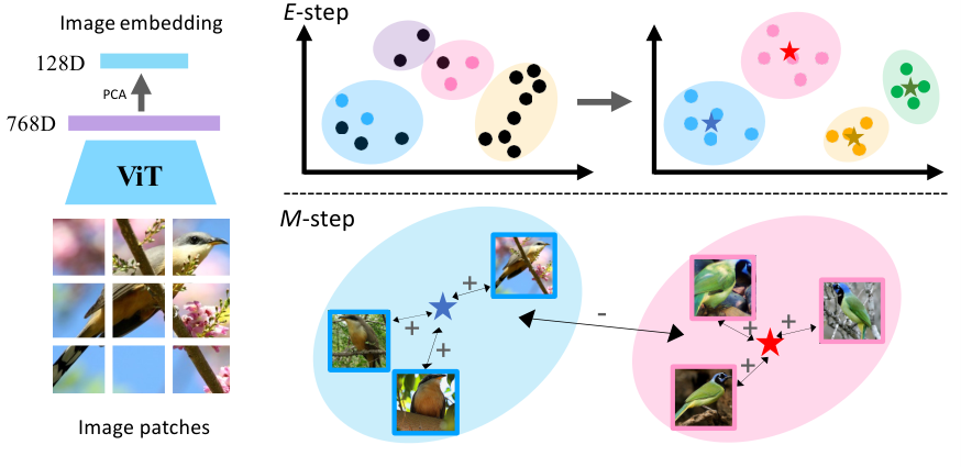
In this paper, we argue that representation learning and the estimation of class numbers should be considered together and could reinforce each other, i.e., a strong representation could help a more accurate estimation of the class numbers, and an accurate class number could help learn a better feature representation. To this end, we propose a unified EM-like framework that alternates between feature representation learning and class number estimation where the E-step is aimed at automatically estimating a proper class number and a set of class prototypes in the unlabelled data and the M-step is aimed at learning better representation with the class number and class prototypes estimated. In particular, we propose using a prototype contrastive representation learning [29] method for GCD, which requires a set of prototypes to serve as anchors for representation learning. Prototypical contrastive learning [29] is developed for unsupervised representation learning to generalize to different tasks, where the prototypes are obtained by over-clustering the dataset with one or multiple given prototype numbers, using non-parametric clustering algorithms like -means. Instead, to handle the problem of GCD, we propose to estimate the prototype number and prototypes automatically and simultaneously. To do so, we introduce a semi-supervised variant of the Gaussian Mixture Model (GMM) with a stochastic splitting and merging mechanism to determine the most suitable clusters based on current representation. These clusters can then be used to form prototypes to facilitate contrastive representation learning. Our framework alternates between the E- and M-step until converging to achieve robust representation and reliable category estimation. After learning, the cluster assignment for an unlabelled instance, either from known or novel classes, can be retrieved by finding the nearest prototypes. Thus we name our framework as GPC: Gaussian mixture model for generalized category discovery with Protypical Contrastive learning.
Our contributions in this paper are as follows: (1) We demonstrate that in generalized category discovery, the class number estimation and representation learning can reinforce each other in the learning process. Strong representations can give a better estimation of the class number, and vice versa. (2) We propose an EM-like framework that alternates between prototype estimation with a variant of GMM (E-step) and representation learning based on prototypical contrastive learning (M-step). (3) We introduce a semi-supervised variant of GMM with a stochastic splitting and merging mechanism to allow dynamic change of the prototypes by examining the cluster compactness and separability based on the Metropolis-Hastings ratio [17]. (4) We comprehensively evaluated our framework on both the generic image classification benchmark, including CIFAR10, CIFAR100, ImageNet-100, and the challenging fine-grained Semantic Shifts Benchmark suite, which includes CUB-200, Stanford-Cars, and FGVC-aircrafts, achieving the state-of-the-art results.
2 Related work
Novel category discovery (NCD) is first formalized in DTC [16], where the task is to discover new categories leveraging the knowledge of a set of labelled categories. Earlier methods like MCL [20] and KCL [21] for generalized transfer learning can also be applied to this problem. RankStat [14, 15] shows that this task benefits from self-supervised pretraining and proposes a method to transfer knowledge from the labelled data to the unlabelled data using ranking statistics. NCL [56] and [24] adopt contrastive learning for novel category discovery. OpenMix [57] shows that mixing up labelled and unlabelled data can help avoid the representation from overfitting to the labelled categories. [54] propose a dual ranking statistics framework to focus on the local visual cues to improve the performance on fine-grained classification benchmarks. UNO [12] introduces a unified cross-entropy loss that enables the model to be jointly trained on unlabelled and labelled data. Most recently, generalized category discovery (GCD) is introduced in [45] to extend NCD to a more open-world setting where unlabelled instances can come from both labelled and unlabelled categories. Concurrent work ORCA [2] also tackles a similar setting as GCD, termed open-world semi-supervised learning. Later works [11, 48, 35, 53] extends on the GCD setting and proposed more effective methods, some works also explored the incremental setting of the GCD problem [55, 39] Despite the advance in this setting, most methods still assume that the novel class number is known a priori, which is often not the case in the real world. To address this problem, DTC [16] and GCD [45] precompute the number of novel classes using a semi-supervised -means algorithm, without considering the representation learning. In this paper, we demonstrate that class number estimation and representation learning can be jointly considered to mutually benefit each other.
Contrastive learning [4, 5, 18, 7, 58] (CL) has been shown very effective for representation learning in a self-supervised manner, using the instance discrimination pretext [49] as the learning objective. The instance discrimination task learns a representation by pulling positive samples from the augmentations of the same images closer and pushing negative samples from different images apart in the embedding space. Instead of contrasting over all instances in a mini-bath, prototypical contrastive learning (PCL) [29] proposes to contrast the features with a set of prototypes which can provide a higher level abstraction of dataset than instances and has been shown to be more data efficient without the need of large batch size. Though PCL is developed for unsupervised representation learning, if the prototypes are viewed as cluster centers, it can be leveraged in the partially supervised setting of GCD for representation learning to better fit the GCD task of partitioning data into different clusters. Thus, in this paper, we adopt PCL to fit the GCD setting for representation learning in which the downstream clustering task is directly considered.
Semi-supervised learning (SSL) has been a long standing research topic which many effective method proposed [36, 41, 1, 28, 43]. In SSL, the labelled and the unlabelled data are assumed to come from the same set of classes, and the task is to learn a classification model that can take advantage of both labelled and unlabelled data. Consistency-based methods are among the most effective methods for SSL, such as Mean-teacher [43], MixMatch [1], and FixMatch [41]. Self-supervised representation learning also shows to be helpful for SSL because it can provide a strong representation [52, 36]. Recent works extend semi-supervised learning by relaxing the assumption of exactly the same classes in the labeled and unlabelled data [40, 23, 51], but their focus is improving the performance of the labeled categories without discovering novel categories in the unlabeled set.
Unsupervised clustering has been studied for decades, and there are many existing classical approaches [31, 10, 6] as well as deep learning based approaches [50, 37, 13]. Recently, DeepDPM [38] is proposed to automatically determine the number of clusters for a given dataset by adopting a similar split/merge framework that changes the inferred number of clusters. However, due to the unsupervised nature of these methods, there is no prior or supervision over how a cluster should be formed, thus multiple equally valid clustering results following different clustering criteria can be produced. Thus, directly applying unsupervised clustering methods to the task of generalized category discovery is not feasible, as we would want the model to use one unique clustering criteria implicitly given by the labelled data.
3 Method
Given a collection of partially labelled data, , where is labelled, is unlabelled, and , Generalized category discovery (GCD) aims at automatically assign labels for the unlabelled instances in , by transferring knowledge acquired from . Let the category number in be and that in be . The number of new categories is then . Though can be accessed from the labelled data, we do not assume or to be known. This is a realistic setting to reflect the real open world, where we often have access to some labelled data, but in the unlabelled data, we also have instances from unseen new categories.
The key challenges for GCD are representation learning, category number estimation, and label assignment. Existing methods for NCD and GCD [16, 45] deal with these three challenges independently. However, we believe they are inherently linked with each other. Label assignment depends on representation and category number estimation. A good class number estimation can facilitate representation learning, thus better label assignment, and vice versa. Thus, in this paper, we aim to jointly handle these challenges in the learning process for a more reliable GCD.
To this end, we propose a unified EM-like framework that alternates between representation learning and class number estimation, while the label assignment turns out to be a by-product during class number estimation. In the E-step, we introduce a semi-supervised variant of the Gaussian Mixture Model (GMM) to estimate the class numbers by dynamically splitting separable clusters and merging cluttered clusters based on current representation, forming a set of class prototypes for both seen and unseen classes, and in the M-step, we train the model to produce discriminative representation by prototypical contrastive learning using the cluster centers from the GMM prototypes derived from the E-step during class number estimation. After training, the class assignment for each instance can be retrieved by simply identifying the nearest prototype.
3.1 Representation learning
The goal of representation learning is to learn a discriminative representation that can well separate different categories, not only the old ones, but also the new ones. Contrastive learning (CL) has been shown to be an effective choice for NCD [24] and GCD [45]. Self-supervised contrastive learning is defined as
| (1) |
where and are the representations of two views obtained from the same image using random augmentations and is the temperature. Two views of the same instance are pulled closer, and different instances are pushed away during training. Self-supervised contrastive learning and its supervised variant, in which different instances from the same category are also pulled closer, are used in [45] for representation learning. However, as a stronger training signal is used for the labelled data, the representation is likely biased to the labelled data to some extent. Moreover, such a method does not take the downstream clustering task into account during learning, thus a clustering algorithm is required to run independently after the representation learning.
In this paper, we adopt prototypical contrastive learning (PCL) [29] to the GCD setting to learn the representation . PCL uses a set of prototypes to represent the dataset for contrastive learning instead of the random augmentation generated views . PCL loss can be written as
| (2) |
where is the corresponding prototype for . It was originally designed as an alternative for self-supervised contrastive learning by over-clustering the training data to obtain the prototypes during training. We employ PCL here to learn reliable representation while taking the downstream clustering into account for GCD, where we have a set of partially labelled data. In our case, the prototypes can be interpreted as the class centers for each of the categories. To obtain the prototypes for the seen categories, we directly calculate the class mean by averaging all the feature vectors of the labelled instances. For the unseen categories, we obtain the prototypes with a semi-supervised variant of the Gaussian Mixture Model (GMM), as will be introduced in Section 3.2. This way, the cluster assignment for an unlabelled image can be readily achieved by finding the nearest prototype.
Additionally, we observe that only a few principal dimensions can already recover most of the variances in the representation space of , which is known as dimensional collapse (DC) in [25, 22], and it is shown that DC can be caused by strong augmentations or implicit regularizations in the model, and preventing DC during training can lead to a better feature representation. To alleviate DC for representation learning in our case, we propose to first project the feature to a subspace obtained by principal component analysis (PCA) before the contrastive learning. Specifically, we apply PCA on a matrix formed by a mini-batch of features , with a batch size of , the feature dimension , and the number of effective principal directions . We have , where , and . We can then project features to principal directions to obtain a more compact feature , and replace feature with in Eq. 2 for PCL. The prototypes are also computed in the projected space.
We jointly use self-supervised contrastive learning and PCL to train our model. The overall learning objective can be written as
| (3) |
where is a linear warmup function defined as where is the current epoch and warmup length ( in our experiments). The reason we use both CL and PCL is that, in the beginning, the representation is not well suited for clustering, and thus the obtained prototypes are not informative to facilitate the representation learning. Hence, we gradually increase the weight of PCL during training from 0 to 1 in the first epochs.

3.2 Class number and prototypes estimation with semi-supervised Gaussian mixture model
In this section, we present a semi-supervised variant of the Gaussian mixture model (GMM) with each Gaussian component consisting of two sub-components to estimate the prototypes for representation learning in Section 3.1 and the unknown class number. GMM estimates the prototypes and assigns a label for each data point by finding its nearest prototype. The cluster label assignment and the prototypes are then used for prototypical contrastive learning. The GMM is defined as
| (4) |
where is the Gaussian probability density function with mean and covariance , and is the weight for -th Gaussian component and we have . Ideally, we would expect the component number in the GMM to be equal to the class number in . To estimate the unknown class number , we leverage an automatic splitting-and-merging strategy into the modeling process to obtain an optimal , which is expected to be as close to as possible. We alternate between representation learning and estimation until convergence to get discriminative representation learning and a reliable class number estimation. For initialization, can be set to any number greater than . In our experiments, we simply set the initial number of components to a default . We run a semi-supervised -means algorithm [45] with to obtain the and for each component in the mixture model. Note that the semi-supervised -means algorithm is constrained to the labelled data in a way that labelled instances from the same class are assigned to the same cluster, and labelled instances from different classes will not be assigned to the same cluster. To facilitate the splitting and merging process, for each Gaussian component defined by and , we further depict it with a GMM with two sub-components and with . We run a -means with on the -th component to obtain and .
| , , and | The datasets. |
| Initial guess of . |
for to do 2
For a cluster whose two sub-components are roughly independent and equally sized (e.g., left part of Fig. 2), i.e., they are easily separable, we would like the model to split it into two such that the model can better fit the data distribution and the class assignment will be more accurate because it is less likely that such distinct clusters will belong to the same class. For two clusters that are cluttered with each other (e.g., right part of Fig. 2), i.e., difficult to distinguish, we would like to merge them into one, so that they will be considered as from the same class. Following this intuition, we use the Metropolis-Hastings framework [17] to compute a probability to stochastically split a cluster into two. The Hastings ratio is defined as
| (5) |
where is the factorial function, i.e., , is the set of data points in cluster , is the set of data points in the -th sub-cluster of cluster , , , is the marginal likelihood of the observed data by integrating out the and parameters in the Gaussian, and is the prior distribution of and . More details can be found in the supplementary. The intuition behind this is that, if the number of data points in two sub-components is roughly balanced, which is measured by the terms, and the data points in the two sub-components are independent of each other, which is measure by the terms, there should be a greater chance of splitting the cluster. After performing a split operation, the and of previous components will be replaced with and of two sub-components. We will then run two -means within the two newly formed components to obtain their corresponding sub-components. On the contrary, if two clusters are cluttered with each other, they should be merged. Similar to splitting, we determine the merging probability by , where is calculated similarly for two clusters and :
| (6) |
Note that both and are within the range of , so we use and to convert it into a valid probability.
To take the labelled instances into consideration during the splitting-and-merging process, if a cluster consists of labelled instances, we set its ; if for any two clusters containing instances from two labelled classes, we set their .
During the splitting-and-merging process, we first apply splitting according to the and then apply merging according to . The newly formed clusters by splitting will not be reused during the merging step. After finishing the splitting and merging, we can obtain the prototypes, and thus can estimate , for our PCL-based representation learning. We alternate between representation learning and class number estimation for each training epoch until converge. The final will be considered the estimated class number in . The cluster assignment for each unlabelled instance can be easily retrieved by identifying its nearest prototype, without the need of running a non-parametric clustering algorithm as [45]. The overall training process is summarized in Algorithm 1.
| CIFAR10 | CIFAR100 | ImageNet-100 | ||||||||||
| No. | Methods | Known | PCA | All | Old | New | All | Old | New | All | Old | New |
| (1) | -means [31] | ✓ | ✗ | 83.6 | 85.7 | 82.5 | 52.0 | 52.2 | 50.8 | 72.7 | 75.5 | 71.3 |
| (2) | RankStats+ [15] | ✓ | ✗ | 46.8 | 19.2 | 60.5 | 58.2 | 77.6 | 19.3 | 37.1 | 61.6 | 24.8 |
| (3) | UNO+ [12] | ✓ | ✗ | 68.6 | 98.3 | 53.8 | 69.5 | 80.6 | 47.2 | 70.3 | 95.0 | 57.9 |
| (4) | ORCA [2] | ✓ | ✗ | 81.8 | 86.2 | 79.6 | 69.0 | 77.4 | 52.0 | 73.5 | 92.6 | 63.9 |
| (5) | Vaze et al. [45] | ✓ | ✗ | 91.5 | 97.9 | 88.2 | 73.0 | 76.2 | 66.5 | 74.1 | 89.8 | 66.3 |
| (6) | Ours (GPC) | ✓ | ✗ | 92.0 | 98.3 | 88.7 | 77.4 | 84.8 | 62.4 | 76.5 | 94.0 | 68.5 |
| (7) | Ours (GPC) | ✓ | ✓ | 92.2 | 98.2 | 89.1 | 77.9 | 85.0 | 63.0 | 76.9 | 94.3 | 71.0 |
| (8) | Vaze et al. [45] | ✗ | ✗ | 88.6 | 96.2 | 84.9 | 73.2 | 83.5 | 57.9 | 72.7 | 91.8 | 63.8 |
| (9) | Vaze et al. [45] | ✗ | ✓ | 89.7 | 97.3 | 86.3 | 74.8 | 83.8 | 58.7 | 73.8 | 92.1 | 64.6 |
| (10) | Ours (GPC) | ✗ | ✗ | 88.2 | 97.0 | 85.8 | 74.9 | 84.3 | 59.6 | 74.7 | 92.9 | 65.1 |
| (11) | Ours (GPC) | ✗ | ✓ | 90.6 | 97.6 | 87.0 | 75.4 | 84.6 | 60.1 | 75.3 | 93.4 | 66.7 |
4 Experimental results
4.1 Experimental setup
Benchmark and evaluation metric.
We validate the effectiveness of our method on the generic image classification benchmark (including CIFAR-10/100 [27] and ImageNet-100 [44]) and also the recently proposed Semantic Shift Benchmark [46] (SSB)(including CUB-200 [47], Stanford Cars [26], and FGVC-Aircraft [32]). For each of the datasets, we follow [45] and sample a subset of all classes for which we have annotated labels during training. For experiments on SSB datasets, we directly use the class split from [46]. 50% of the images from these labelled classes will be used as the labelled instances in , and the remaining images are regarded as the unlabelled data containing instances from labelled and unlabelled classes. See Table 2 for statistics of the datasets we evaluated. We evaluate model performance with clustering accuracy (ACC) following standard practice in the literature. At test-time, given ground truth labels and model predicted cluster assignments , the ACC is calculated as where is the optimal permutation for matching predicted cluster assignment to actual class label and .
| labelled | unlabelled | |
| CIFAR-10 | 5 | 5 |
| CIFAR-100 | 80 | 20 |
| ImageNet-100 | 50 | 50 |
| CUB-200 | 100 | 100 |
| Stanford-Cars | 98 | 98 |
| FGVC-aircraft | 50 | 50 |
Implementation details.
We train and test all the methods with a ViT-B/16 backbone [9] with pretrained weights from DINO [3]. We use the output of [CLS] token with a dimension of 768 as the feature representation for an input image. We only finetune the last block of the ViT-B backbone to prevent the model from overfitting to the labelled classes during training. We set the batch size for training the model to 128 with 64 labelled images and 64 unlabelled images and use a cosine annealing schedule for the learning rate starting from 0.1. The number of principal directions in the PCA is set to 128, which we found performs the best across all the datasets evaluated. We train all the methods for 200 epochs on each dataset for a fair comparison with previous works, and the best-performing model is selected using the accuracy on the validation set of the labelled classes. All experiments are done with an NVIDIA V100 GPU with 32GB memory.
| CUB | Stanford Cars | FGVC-aircraft | ||||||||||
| No. | Methods | Known | PCA | All | Old | New | All | Old | New | All | Old | New |
| (1) | -means [31] | ✓ | ✗ | 34.3 | 38.9 | 32.1 | 12.8 | 10.6 | 13.8 | 16.0 | 14.4 | 16.8 |
| (2) | RankStats+ [15] | ✓ | ✗ | 33.3 | 51.6 | 24.2 | 28.3 | 61.8 | 12.1 | 26.9 | 36.4 | 22.2 |
| (3) | UNO+ [12] | ✓ | ✗ | 35.1 | 49.0 | 28.1 | 35.5 | 70.5 | 18.6 | 40.3 | 56.4 | 32.2 |
| (4) | ORCA [2] | ✓ | ✗ | 35.3 | 45.6 | 30.2 | 23.5 | 50.1 | 10.7 | 22.0 | 31.8 | 17.1 |
| (5) | Vaze et al. [45] | ✓ | ✗ | 51.3 | 56.6 | 48.7 | 39.0 | 57.6 | 29.9 | 45.0 | 41.1 | 46.9 |
| (6) | Ours (GPC) | ✓ | ✗ | 54.2 | 54.9 | 50.3 | 41.2 | 58.8 | 31.6 | 46.1 | 42.4 | 47.2 |
| (7) | Ours (GPC) | ✓ | ✓ | 55.4 | 58.2 | 53.1 | 42.8 | 59.2 | 32.8 | 46.3 | 42.5 | 47.9 |
| (8) | Vaze et al. [45] | ✗ | ✗ | 47.1 | 55.1 | 44.8 | 35.0 | 56.0 | 24.8 | 40.1 | 40.8 | 42.8 |
| (9) | Vaze et al. [45] | ✗ | ✓ | 49.2 | 56.2 | 46.3 | 36.3 | 56.6 | 25.9 | 43.2 | 40.9 | 44.6 |
| (10) | Ours (GPC) | ✗ | ✗ | 50.2 | 52.8 | 45.6 | 36.7 | 56.3 | 26.3 | 39.7 | 39.6 | 42.7 |
| (11) | Ours (GPC) | ✗ | ✓ | 52.0 | 55.5 | 47.5 | 38.2 | 58.9 | 27.4 | 43.3 | 40.7 | 44.8 |
4.2 Comparison with the state-of-the-art
In Table 1, we report the comparison with the state-of-the-art method of [45], strong baselines derived from NCD methods, and the -means on the generic classification datasets. Notably, our method consistently achieves the best overall performance on all datasets, under the challenging setting where the class number is unknown. When the class number is known, our method also achieves the best performance on all datasets, except ImageNet-100, on which the best performance is achieved by ORCA [2]. In rows 1-7, we compare with other methods with the known class number in the unlabelled data, while in rows 8-11 we compare with [45] for the case of the unknown class number. We can see that our proposed framework outperforms other methods in most cases and especially when the number of classes is unknown. Comparing rows 10 and 11 to row 5, we can see that our proposed method without knowing the number of classes can even match the performance of previous strong baseline with the number of classes known to the model. Furthermore, from row 6 vs row 7 and row 10 vs row 11, we can see that the additional PCA layer can effectively improve the performance, also the performance improvement from PCA is larger on the ‘New’ classes than on the ‘Old’ classes, which validates that the PCA can keep the representation space from collapsing and improve the performance on classes without using any labels. Due to the fact that labelled instances provide a stronger training signal, we can see from rows 6 - 11 that performance on ‘Old’ classes is generally steady. Comparing row 7 to row 5 and row 11 to row 8, we can see our full method outperforms the previous state-of-the-art method Vaze et al. [45] by large margins on both known and unknown class number cases. Table 3 shows performance comparison on the more challenging fine-grained Semantic Shift Benchmark [46]. A similar trend of Table 1 holds true for the results on SSB. Our approach achieves competitive performance in all cases and again reaches a better performance when the number of classes is unknown. In Table 4, we present the results on the Herbarium-19 dataset which is a long-tailed dataset, adding additional challenges for the GCD task. Again, our method performs the best on ‘All’ and ‘New’ classes. These results demonstrate the effectiveness of our method.
| Methods | All | Old | New |
| -means [31] | 13.0 | 12.2 | 13.4 |
| RS+ [15] | 27.9 | 55.8 | 12.8 |
| UNO+ [12] | 28.3 | 53.7 | 14.7 |
| ORCA [2] | 20.9 | 30.9 | 15.5 |
| GCD [45] | 35.4 | 51.0 | 27.0 |
| Ours (GPC) | 36.5 | 51.7 | 27.9 |
4.3 Novel class number estimation
One of the important yet overlooked components in the NCD and GCD literature is the estimation of unknown class numbers. Our proposed framework leverages a modified GMM to estimate the class number, in which we need to define an initial guess of the class number. We validate the effects of different choices of the initial guess w.r.t. the estimated class number in Table 5. Note that the number in Table 5 is . We can see that our proposed framework is generally robust to a wide range of initial guesses. We found that is a simple and reliable choice. Hence we use this for all datasets.
| Dataset | GT | Vaze et al.[45] | 3 | 5 | 10 | 20 | 30 | 50 | 100 | |
| CIFAR-10 | 5 | 5 | 4 | 5 | 5 | 5 | 6 | 6 | 8 | 14 |
| CIFAR-100 | 80 | 20 | 20 | 16 | 20 | 20 | 21 | 22 | 27 | 36 |
| ImageNet-100 | 50 | 50 | 59 | 58 | 48 | 57 | 55 | 54 | 50 | 60 |
| CUB | 100 | 100 | 131 | 79 | 87 | 86 | 88 | 92 | 112 | 101 |
| SCars | 98 | 98 | 132 | 84 | 90 | 86 | 87 | 89 | 115 | 104 |
4.4 Training complexity
Given that our framework necessitates the fitting of GMMs, an extended training duration is required. We compare the performance of our method to the extended method of Vaze et al. [45], which is pushed to its original number of training epochs. The results in Table 6 demonstrate that our method outperforms [45] across both CUB and ImageNet-100 datasets while maintaining a similar training duration. Furthermore, in contrast to the baseline method, our approach eliminates the need for additional post-training procedures such as running SS--means on the entire dataset for label assignment.
| Method | CUB | ImageNet-100 | ||||
| All | Old | New | All | Old | New | |
| Vaze et al. [45] | 51.3 | 56.6 | 48.7 | 74.1 | 89.8 | 66.3 |
| Vaze et al.(1.5) | 52.0 | 56.8 | 49.0 | 74.7 | 90.3 | 66.7 |
| GPC | 55.4 | 58.2 | 53.1 | 76.9 | 94.3 | 71.0 |
4.5 Ablation study
Number of dimensions in PCA
The PCA in our framework requires setting a number for the number of principal directions to extract from data. In Fig. 3, we show the results of using a different number of principal directions in PCA on CUB-200 and ImageNet-100 datasets. We can see from Fig. 3(a) that for both datasets, 128 principal directions can already explain most of the variances in the data, thus we choose the PCA dimension to be 128 for all our experiments. We further experiment with other different choices of the PCA dimension and shows the result in Fig. 3(b), which again confirms that 128 principal directions are already expensive enough, and obtain the best performance over other choices, that are either too few or too many, effectively avoiding DC.
Different methods for prototype estimation
Our semi-supervised GMM plays an important role in prototype estimation for representation learning based on prototypical contrastive learning. Here, we replace our semi-supervised GMM with other alternatives that do not produce prototypes automatically. Particularly, we compare our method with DBSCAN [10], Agglomerative clustering [33], and semi-supervised -means [16, 45]. The prototypes are then obtained by averaging the data points that are assigned to the same cluster. For a fair comparison, the same regulations to prevent the wrong clustering results for labelled instances are applied to all methods, i.e., during the clustering process, two labelled instances with the same label will fall into the same cluster, and two instances with different labels will be assigned to different clusters. The results are reported in Table 7(a). Our method achieves the best performance on all three datasets, indicating that better prototypes are obtained by our approach to facilitate representation learning. Note that DBSCAN requires two important user-defined parameters, radius, and minimum core points, the ideal values of which lack a principled way to obtain in practice, while our method is parameter-free and can seamlessly be combined with the representation learning to jointly enhance each other, obtaining better performance.
Combining our GMM with other GCD methods
We further combine our semi-supervised GMM with automatic splitting and merging with other methods, allowing joint representation learning and category discovery without a predefined category number. As the state-of-the-art GCD method [45] does not contain any parametric classifier during representation, so it can be directly combined with our GMM. For the RankStat and the DualRank methods that have a parametric classifier for category discovery, we treat the weights of the classifier as the cluster centers and run our GMM to automatically determine the category number during representation learning. The results are presented in Table 7(b). Comparing with row 9 in Table 1 and Table 3, we can see using our GMM can also improve [45] on CUB and Stanford Cars, while our proposed framework consistently achieves better performance on all datasets, again validating that our design choices.
Class number estimation with different representations
Here, we validate our class number estimation method on top of the representations learned by other GCD approaches and report the results in Table 8. It can be seen, applying our method on other GCD representations can achieve reasonably well results. Notably, by applying our class number estimation method on top of the representation by the existing state-of-the-art method, we can obtain better class number estimation results, though the overall best results are obtained with the representation learned in our framework.
| Representation | C-100 | CUB | SCars | IM-100 |
| Ground Truth | 20 | 100 | 98 | 50 |
| Vaze et al.[45] | 20 | 131 | 132 | 59 |
| Ours w/ [15] feat. | 19 | 111 | 94 | 55 |
| Ours w/ [54] feat. | 22 | 116 | 89 | 49 |
| Ours w/ [45] feat. | 21 | 121 | 109 | 57 |
| Ours (GPC) | 20 | 112 | 103 | 53 |
Partial overlap between and
We evaluate the performance of our method when we relax to , i.e., the two sets may only partially overlap. We vary the number of overlapped classes and report the results in Table 9.
Our approach consistently outperforms the method proposed by Vaze et al. [45] in all configurations. These compelling results not only showcase the robustness of our method but also highlight its effectiveness in scenarios involving partial overlap between known and unknown classes.
| 25 | 50 | 75 | |||||||
| All | Old | New | All | Old | New | All | Old | New | |
| Vaze et al. [45] | 49.5 | 50.1 | 48.2 | 51.2 | 50.7 | 52.2 | 52.7 | 50.9 | 54.5 |
| Ours | 51.2 | 52.6 | 49.5 | 52.3 | 51.6 | 54.8 | 53.6 | 51.4 | 55.9 |
Varying ratio of Old/New categories
We measure the estimated new class numbers when varying the ratio of Old/New categories while having on CUB in Table 10. As can be seen, for all cases, our method outperforms [45]. Meanwhile, we can also see that when the initial guess is too far from the ground truth, the estimation will be less accurate.
| Old/New | 20/180 | 40/160 | 60/140 | 80/120 |
| GCD [45] | 87 | 102 | 114 | 104 |
| Ours | 93 | 126 | 135 | 116 |
5 Conclusion
In this paper, we present an EM-like framework for the challenging GCD problem without knowing the number of new classes, with the E-step automatically determining the class number and prototypes and the M-step being robust representation learning. We introduce a semi-supervised variant of GMM with a stochastic splitting and merging mechanism to obtain the prototypes and leverage these evolving prototypes for representation learning by prototypical contrastive learning. We demonstrated that class number estimation and representation learning can facilitate each other for more robust category discovery. Our framework obtains state-of-the-art performance on multiple public benchmarks.
Acknowledgements
This work is supported by Hong Kong Research Grant Council - Early Career Scheme (Grant No. 27208022) and HKU Seed Fund for Basic Research.
References
- [1] David Berthelot, Nicholas Carlini, Ian Goodfellow, Nicolas Papernot, Avital Oliver, and Colin Raffel. Mixmatch: A holistic approach to semi-supervised learning. In NeurIPS, 2019.
- [2] Kaidi Cao, Maria Brbić, and Jure Leskovec. Open-world semi-supervised learning. In ICLR, 2022.
- [3] Mathilde Caron, Hugo Touvron, Ishan Misra, Hervé Jégou, Julien Mairal, Piotr Bojanowski, and Armand Joulin. Emerging properties in self-supervised vision transformers. In ICCV, 2021.
- [4] Ting Chen, Simon Kornblith, Mohammad Norouzi, and Geoffrey Hinton. A simple framework for contrastive learning of visual representations. In ICML, 2020.
- [5] Xinlei Chen, Haoqi Fan, Ross Girshick, and Kaiming He. Improved baselines with momentum contrastive learning. arXiv preprint arXiv:2003.04297, 2020.
- [6] Dorin Comaniciu and Peter Meer. Mean shift: A robust approach toward feature space analysis. IEEE TPAMI, 2002.
- [7] Quan Cui, Bingchen Zhao, Zhao-Min Chen, Borui Zhao, Renjie Song, Jiajun Liang, Boyan Zhou, and Osamu Yoshie. Discriminability-transferability trade-off: An information-theoretic perspective. In ECCV, 2022.
- [8] Jia Deng, Wei Dong, Richard Socher, Li-Jia Li, Kai Li, and Li Fei-Fei. Imagenet: A large-scale hierarchical image database. In CVPR, 2009.
- [9] Alexey Dosovitskiy, Lucas Beyer, Alexander Kolesnikov, Dirk Weissenborn, Xiaohua Zhai, Thomas Unterthiner, Mostafa Dehghani, Matthias Minderer, Georg Heigold, Sylvain Gelly, Jakob Uszkoreit, and Neil Houlsby. An image is worth 16x16 words: Transformers for image recognition at scale. In ICLR, 2021.
- [10] Martin Ester, Hans-Peter Kriegel, Jörg Sander, Xiaowei Xu, et al. A density-based algorithm for discovering clusters in large spatial databases with noise. In KDD, 1996.
- [11] Yixin Fei, Zhongkai Zhao, Siwei Yang, and Bingchen Zhao. Xcon: Learning with experts for fine-grained category discovery. In BMVC, 2022.
- [12] Enrico Fini, Enver Sangineto, Stéphane Lathuilière, Zhun Zhong, Moin Nabi, and Elisa Ricci. A unified objective for novel class discovery. In ICCV, 2021.
- [13] Kamran Ghasedi Dizaji, Amirhossein Herandi, Cheng Deng, Weidong Cai, and Heng Huang. Deep clustering via joint convolutional autoencoder embedding and relative entropy minimization. In ICCV, 2017.
- [14] Kai Han, Sylvestre-Alvise Rebuffi, Sebastien Ehrhardt, Andrea Vedaldi, and Andrew Zisserman. Automatically discovering and learning new visual categories with ranking statistics. In ICLR, 2020.
- [15] Kai Han, Sylvestre-Alvise Rebuffi, Sebastien Ehrhardt, Andrea Vedaldi, and Andrew Zisserman. Autonovel: Automatically discovering and learning novel visual categories. IEEE TPAMI, 2021.
- [16] Kai Han, Andrea Vedaldi, and Andrew Zisserman. Learning to discover novel visual categories via deep transfer clustering. In ICCV, 2019.
- [17] Wilfred Keith Hastings. Monte carlo sampling methods using markov chains and their applications. Biometrika, 1970.
- [18] Kaiming He, Haoqi Fan, Yuxin Wu, Saining Xie, and Ross Girshick. Momentum contrast for unsupervised visual representation learning. In CVPR, 2020.
- [19] Kaiming He, Xiangyu Zhang, Shaoqing Ren, and Jian Sun. Deep residual learning for image recognition. In CVPR, 2016.
- [20] Yen-Chang Hsu, Zhaoyang Lv, and Zsolt Kira. Learning to cluster in order to transfer across domains and tasks. In ICLR, 2018.
- [21] Yen-Chang Hsu, Zhaoyang Lv, Joel Schlosser, Phillip Odom, and Zsolt Kira. Multi-class classification without multi-class labels. In ICLR, 2019.
- [22] Tianyu Hua, Wenxiao Wang, Zihui Xue, Yue Wang, Sucheng Ren, and Hang Zhao. On feature decorrelation in self-supervised learning. In ICCV, 2021.
- [23] Junkai Huang, Chaowei Fang, Weikai Chen, Zhenhua Chai, Xiaolin Wei, Pengxu Wei, Liang Lin, and Guanbin Li. Trash to treasure: harvesting ood data with cross-modal matching for open-set semi-supervised learning. In ICCV, 2021.
- [24] Xuihui Jia, Kai Han, Yukun Zhu, and Bradley Green. Joint representation learning and novel category discovery on single-and multi-modal data. In ICCV, 2021.
- [25] Li Jing, Pascal Vincent, Yann LeCun, and Yuandong Tian. Understanding dimensional collapse in contrastive self-supervised learning. In ICLR, 2021.
- [26] Jonathan Krause, Michael Stark, Jia Deng, and Li Fei-Fei. 3d object representations for fine-grained categorization. In 4th International IEEE Workshop on 3D Representation and Recognition (3dRR-13), 2013.
- [27] Alex Krizhevsky and Geoffrey Hinton. Learning multiple layers of features from tiny images. Technical Report, 2009.
- [28] Samuli Laine and Timo Aila. Temporal ensembling for semi-supervised learning. In ICLR, 2017.
- [29] Junnan Li, Pan Zhou, Caiming Xiong, and Steven CH Hoi. Prototypical contrastive learning of unsupervised representations. In ICLR, 2020.
- [30] Mingxuan Liu, Subhankar Roy, Zhun Zhong, Nicu Sebe, and Elisa Ricci. Large-scale pre-trained models are surprisingly strong in incremental novel class discovery. arXiv preprint arXiv:2303.15975, 2023.
- [31] James MacQueen. Some methods for classification and analysis of multivariate observations. In Proceedings of the Fifth Berkeley Symposium on Mathematical Statistics and Probability, 1967.
- [32] Subhransu Maji, Esa Rahtu, Juho Kannala, Matthew Blaschko, and Andrea Vedaldi. Fine-grained visual classification of aircraft. arXiv preprint arXiv:1306.5151, 2013.
- [33] Fionn Murtagh and Pierre Legendre. Ward’s hierarchical agglomerative clustering method: which algorithms implement ward’s criterion? Journal of classification, 2014.
- [34] Avital Oliver, Augustus Odena, Colin Raffel, Ekin D Cubuk, and Ian J Goodfellow. Realistic evaluation of deep semi-supervised learning algorithms. In NeurIPS, 2018.
- [35] Nan Pu, Zhun Zhong, and Nicu Sebe. Dynamic conceptional contrastive learning for generalized category discovery. In CVPR, 2023.
- [36] Sylvestre-Alvise Rebuffi, Sebastien Ehrhardt, Kai Han, Andrea Vedaldi, and Andrew Zisserman. Semi-supervised learning with scarce annotations. In CVPR Deep-Vision workshop, 2020.
- [37] Sylvestre-Alvise Rebuffi, Sebastien Ehrhardt, Kai Han, Andrea Vedaldi, and Andrew Zisserman. Lsd-c: Linearly separable deep clusters. In ICCV Workshop on Visual Inductive Priors for Data-Efficient Deep Learning, 2021.
- [38] Meitar Ronen, Shahaf E. Finder, and Oren Freifeld. Deepdpm: Deep clustering with an unknown number of clusters. In CVPR, 2022.
- [39] Subhankar Roy, Mingxuan Liu, Zhun Zhong, Nicu Sebe, and Elisa Ricci. Class-incremental novel class discovery. In ECCV, 2022.
- [40] Kuniaki Saito, Donghyun Kim, and Kate Saenko. Openmatch: Open-set consistency regularization for semi-supervised learning with outliers. In NeurIPS, 2021.
- [41] Kihyuk Sohn, David Berthelot, Chun-Liang Li, Zizhao Zhang, Nicholas Carlini, Ekin D Cubuk, Alex Kurakin, Han Zhang, and Colin Raffel. Fixmatch: Simplifying semi-supervised learning with consistency and confidence. In NeurIPS, 2020.
- [42] Yiyou Sun and Yixuan Li. Opencon: Open-world contrastive learning. TMLR, 2023.
- [43] Antti Tarvainen and Harri Valpola. Mean teachers are better role models: Weight-averaged consistency targets improve semi-supervised deep learning results. In NeurIPS, 2017.
- [44] Yonglong Tian, Dilip Krishnan, and Phillip Isola. Contrastive multiview coding. In ECCV, 2020.
- [45] Sagar Vaze, Kai Han, Andrea Vedaldi, and Andrew Zisserman. Generalized category discovery. In CVPR, 2022.
- [46] Sagar Vaze, Kai Han, Andrea Vedaldi, and Andrew Zisserman. Open-set recognition: A good closed-set classifier is all you need? In ICLR, 2022.
- [47] Catherine Wah, Steve Branson, Peter Welinder, Pietro Perona, and Serge Belongie. Caltech-UCSD Birds 200. Computation & Neural Systems Technical Report, 2010.
- [48] Xin Wen, Bingchen Zhao, and Xiaojuan Qi. Parametric classification for generalized category discovery: A baseline study. In ICCV, 2023.
- [49] Zhirong Wu, Yuanjun Xiong, Stella X Yu, and Dahua Lin. Unsupervised feature learning via non-parametric instance discrimination. In CVPR, 2018.
- [50] Junyuan Xie, Ross Girshick, and Ali Farhadi. Unsupervised deep embedding for clustering analysis. In ICML, 2016.
- [51] Qing Yu, Daiki Ikami, Go Irie, and Kiyoharu Aizawa. Multi-task curriculum framework for open-set semi-supervised learning. In ECCV, 2020.
- [52] Xiaohua Zhai, Avital Oliver, Alexander Kolesnikov, and Lucas Beyer. S4l: Self-supervised semi-supervised learning. In ICCV, 2019.
- [53] Sheng Zhang, Salman Khan, Zhiqiang Shen, Muzammal Naseer, Guangyi Chen, and Fahad Khan. Promptcal: Contrastive affinity learning via auxiliary prompts for generalized novel category discovery. In CVPR, 2023.
- [54] Bingchen Zhao and Kai Han. Novel visual category discovery with dual ranking statistics and mutual knowledge distillation. In NeurIPS, 2021.
- [55] Bingchen Zhao and Oisin Mac Aodha. Incremental generalized category discovery. In ICCV, 2023.
- [56] Zhun Zhong, Enrico Fini, Subhankar Roy, Zhiming Luo, Elisa Ricci, and Nicu Sebe. Neighborhood contrastive learning for novel class discovery. In CVPR, 2021.
- [57] Zhun Zhong, Linchao Zhu, Zhiming Luo, Shaozi Li, Yi Yang, and Nicu Sebe. Openmix: Reviving known knowledge for discovering novel visual categories in an open world. In CVPR, 2021.
- [58] Rui Zhu, Bingchen Zhao, Jingen Liu, Zhenglong Sun, and Chang Wen Chen. Improving contrastive learning by visualizing feature transformation. In ICCV, 2021.
Appendix A Details of the framework for splitting and merging clusters
In this section, we provide details for the Metropolis-Hastings framework. In the Gaussian Mixture Model, we have three sets of parameters, where is the mixture weight and are the mean and covariance matrix. These parameters are assumed to be sampled from a prior distribution. When and are unknown for the multivariate Gaussian distribution, we adopt the Normal Inverse Wishart (NIW) distribution as the prior to sample them for algebraic convenience, because NIW distribution is a conjugate prior and the conjugacy property can lead to a closed-form expression of the posterior.
The Inverse Wishart (IW) distribution is defined as follows:
| (7) |
where is a Symmetric and Positive Definite(SPD) matrix, , is SPD, and is a -dimensional multivariate factorial function. The positive real number and the SPD matrix are the parameters of the IW distribution. The data distribution determined by and follows NIW distribution, if the joint probability density function is defined by
| (8) |
where , , and is a -dimensional Gaussian with mean and covariance evaluated at .
Given a set of features (with ) assigned to the Gaussian component , we can have a posterior distribution of in a closed-form thanks to the conjugacy:
| (9) |
where the posterior parameters are obtained by:
| (10) | ||||
| (11) | ||||
| (12) | ||||
| (13) |
In Eq.5 and 6 of the main paper, we need to calculate the marginal likelihood function of the observed data by integrating out the and parameters in the Gaussian. Let be the parameters of the NIW distribution. The marginal likelihood can be defined as follows:
| (14) | ||||
| (15) |
with which we can compute the Eq. 5 and 6 in the main paper.
Appendix B Estimating the number of clusters on validation set
In this section, we validate the choice of using only the labelled data, to better reflect the real world use case. In particular, we further split the classes in the labelled data into two parts, and . We drop the labels in . We verify the effectiveness of different choice of on and report the results in Table 11. Interestingly, we observe that the initial guess of a number around often leads to a good estimate.
| Dataset | GT | 1 | 3 | 5 | 10 | 20 | 25 | 50 | |
| CIFAR-10 | 3 | 2 | 2 | 2 | 4 | 5 | 3 | 6 | 8 |
| CIFAR-100 | 60 | 20 | 15 | 18 | 18 | 20 | 21 | 22 | 29 |
| ImageNet-100 | 25 | 25 | 18 | 19 | 22 | 21 | 23 | 27 | 29 |
| CUB | 50 | 50 | 38 | 37 | 41 | 46 | 49 | 52 | 50 |
| SCars | 49 | 49 | 39 | 38 | 40 | 42 | 43 | 48 | 51 |
Appendix C Convergence of the estimated class number in longer training
Here we show results by training the model for 800 epochs on CUB, demonstrating the convergence after longer training.
| Epoch | 200 | 400 | 600 | 700 | 720 | 740 | 760 | 780 | 800 |
| GT | 112 | 122 | 114 | 108 | 109 | 107 | 108 | 106 | 107 |
Appendix D Error bars for generalized category discovery performance
We repeatedly run our method and the previous state-of-the-art three times with different random seeds to show the mean and standard deviation values in Table 13 and Table 14, for both known and unknown class number cases. We can see that the variation is relatively small for all methods, and our method consistently outperforms the previous state-of-the-art across the board for both known and unknown class number cases.
| CIFAR10 | CIFAR100 | ImageNet-100 | ||||||||||
| No. | Methods | Known | PCA | All | Old | New | All | Old | New | All | Old | New |
| (1) | Vaze et al. [45] | ✓ | ✗ | 91.50.4 | 97.90.2 | 88.20.6 | 76.90.3 | 84.60.3 | 61.50.2 | 75.00.3 | 92.10.2 | 66.60.4 |
| (2) | Ours (GPC) | ✓ | ✗ | 91.90.2 | 98.20.3 | 88.60.1 | 77.60.4 | 84.90.4 | 62.70.4 | 76.70.4 | 94.30.2 | 68.80.3 |
| (3) | Ours (GPC) | ✓ | ✓ | 91.90.4 | 98.20.3 | 89.10.2 | 77.80.3 | 85.30.2 | 63.50.2 | 77.30.4 | 94.60.4 | 71.10.3 |
| (4) | Vaze et al. [45] | ✗ | ✗ | 88.60.5 | 96.20.4 | 84.90.6 | 73.20.4 | 83.50.4 | 57.90.4 | 72.70.4 | 91.80.5 | 63.80.6 |
| (5) | Vaze et al. [45] | ✗ | ✓ | 89.70.4 | 97.30.5 | 86.30.4 | 74.80.5 | 83.80.4 | 58.70.6 | 73.80.4 | 92.10.5 | 64.60.6 |
| (6) | Ours (GPC) | ✗ | ✗ | 88.20.4 | 97.00.5 | 85.90.3 | 75.10.5 | 84.40.4 | 59.90.6 | 74.90.5 | 93.20.4 | 65.50.3 |
| (7) | Ours (GPC) | ✗ | ✓ | 90.60.3 | 98.20.4 | 87.10.4 | 75.70.5 | 84.70.6 | 60.90.4 | 75.70.3 | 93.40.4 | 66.80.5 |
| CUB | Stanford Cars | FGVC-aircraft | ||||||||||
| No. | Methods | Known | PCA | All | Old | New | All | Old | New | All | Old | New |
| (1) | Vaze et al. [45] | ✓ | ✗ | 51.10.2 | 56.40.1 | 48.40.3 | 39.10.3 | 57.60.4 | 29.90.3 | 45.10.2 | 41.20.3 | 46.80.2 |
| (2) | Ours (GPC) | ✓ | ✗ | 54.50.2 | 54.60.4 | 50.30.2 | 42.00.2 | 58.90.2 | 32.00.3 | 46.30.2 | 42.30.2 | 47.10.3 |
| (3) | Ours (GPC) | ✓ | ✓ | 55.30.4 | 58.10.3 | 53.20.4 | 42.70.3 | 60.00.4 | 33.00.2 | 46.50.3 | 42.80.5 | 47.20.1 |
| (4) | Vaze et al. [45] | ✗ | ✗ | 47.20.4 | 55.10.3 | 44.80.2 | 35.00.3 | 56.00.4 | 24.80.3 | 40.10.2 | 40.80.4 | 42.80.1 |
| (5) | Vaze et al. [45] | ✗ | ✓ | 49.20.3 | 56.20.2 | 46.30.4 | 36.30.3 | 56.60.4 | 25.90.5 | 41.20.3 | 40.90.4 | 44.60.2 |
| (6) | Ours (GPC) | ✗ | ✗ | 50.50.3 | 52.50.4 | 45.80.5 | 37.00.6 | 56.60.3 | 26.10.2 | 39.80.3 | 39.70.2 | 42.50.2 |
| (7) | Ours (GPC) | ✗ | ✓ | 52.10.3 | 55.40.2 | 45.70.3 | 38.90.4 | 58.90.3 | 28.60.5 | 43.40.3 | 40.80.4 | 44.70.3 |
Appendix E Error bars for category number estimation
In this section, we show the estimated category numbers’ standard deviations by repeatedly running our method with different random seeds. The results are shown in Table 15. We can see that our method can estimate a more accurate category number to Vaze et al. [45].
| Estimated | CIFAR-10 | CIFAR-100 | ImageNet-100 | CUB-200 | Stanford-Cars |
| Ours (GPC) | 51.4 | 222.6 | 543.1 | 1104.2 | 1043.4 |
| Vaze et al. [45] | 41.2 | 231.5 | 594.3 | 1315.6 | 1322.5 |
| Ground Truth | 5 | 20 | 50 | 100 | 98 |
Appendix F Further comparison with ORCA
ORCA [2] is originally pretrained only on the target dataset , i.e., the data that our model is trained on. We have shown the comparison using ImageNet pretrained features from DINO [3] for both ORCA [2] and our method in the main paper. In Table 16 and Table 17, we provide additional comparison with ORCA, showing the effects of pretrained models using different data.
| CIFAR10 | CIFAR100 | ImageNet-100 | |||||||||
| No. | Methods | Pretrain | All | Old | New | All | Old | New | All | Old | New |
| (1) | ORCA [2] | ImageNet | 91.4 | 88.0 | 91.2 | 68.9 | 76.1 | 46.6 | 79.8 | 93.6 | 74.9 |
| (2) | Ours (GPC) | ImageNet | 92.0 | 98.3 | 88.7 | 77.4 | 84.8 | 62.4 | 76.5 | 94.0 | 68.5 |
| (3) | ORCA [2] | Target | 90.6 | 87.2 | 90.1 | 64.7 | 73.2 | 42.1 | 78.7 | 93.4 | 72.4 |
| (4) | Ours (GPC) | Target | 91.1 | 87.8 | 90.5 | 65.0 | 74.3 | 42.6 | 79.6 | 93.3 | 73.1 |
| CUB | SCars | FGVC-Aircraft | |||||||||
| No. | Methods | Pretrain | All | Old | New | All | Old | New | All | Old | New |
| (1) | ORCA [2] | ImageNet | 45.2 | 57.2 | 29.7 | 37.0 | 68.2 | 22.6 | 47.1 | 45.3 | 42.3 |
| (2) | Ours (GPC) | ImageNet | 54.2 | 54.9 | 50.3 | 41.2 | 58.8 | 31.6 | 46.1 | 42.4 | 47.2 |
| (3) | ORCA [2] | Target | 42.9 | 52.0 | 28.4 | 40.3 | 57.0 | 31.4 | 44.4 | 40.7 | 44.1 |
| (4) | Ours (GPC) | Target | 45.0 | 54.2 | 29.1 | 41.2 | 57.1 | 32.1 | 46.2 | 41.0 | 45.2 |
Appendix G Qualitative results
In this section, we provide the visualization of the images grouped using the DINO features and our GPC trained features. The results are presented in each row of Fig. 4 and Fig. 5. The DINO features are effective to some extent when grouping images, but the results are still not satisfactory as the features are not tuned on the downstream tasks with a clear objective (see Fig. 4). On the other hand, after tuning the representation using our method, images from the same category can be grouped together (see Fig. 5).


We also present t-SNE projections of the learned features on both CUB-200 and ImageNet-100 datasets. From Fig. 6 we can see that on CUB-200, the DINO features can not separate different categories very well, while our method and [45] can have a clear category boundary. From Fig. 7, we found that although the t-SNE projections on ImageNet-100 appear to be similarly discriminative among DINO, [45], and our method, while further finetuning the representation from DINO can significantly improve the performance for the task of GCD.

Appendix H Limitation and negative societal impact
It should noted that although our method achieves the state-of-the-art results on the task of generalized category discovery, the classification performance is still far from those models trained with full human supervision. Furthermore, when the class number is unknown, there is still a noticeable performance gap w.r.t. the unknown category number case. Besides, real-world data is much more complex and difficult than the curated data we used. Therefore, careful validation and adaptation to specific application scenarios should be tested before deploying the model for any real-world use.
Appendix I License of used datasets
All the datasets used in this paper are permitted for research use. CIFAR-10 and CIFAR-100 datasets [27] are released under the MIT license, allowing use for research purposes. The terms of access of the ImageNet dataset [8] allow the use for non-commercial research and educational purposes. Similar to ImageNet, the Stanford Cars [26] allows the use for research purposes. The FGVC aircraft [32] dataset was made available exclusively for non-commercial research purposes by the authors. The CUB-200 [47] dataset also allows research use.