Direct measurement of a spatially varying thermal bath using Brownian motion

Micro-mechanical resonators are at the heart of many technologies, including inertial sensing Passaro et al. 2017; Krause et al. 2012, microscopy Giessibl 2003; Poggio and Degen 2010 and bio-sensing Degen et al. 2009; Arlett et al. 2011. Simultaneously, these devices are found to be a paramount tool in fundamental science research, e.g. quantum solid-state experiments Bleszynski-Jayich et al. 2009, optomechanical quantum information experiments Andrews et al. 2014; Wallucks et al. 2020; Barzanjeh et al. 2022, gravity measurements Schmöle et al. 2016; Liu et al. 2021 and dark matter searches Carney et al. 2021. Because both technological applications and pure scientific studies occur at finite temperature, at all times there is a competition between the desired signal source and the typically undesired excitations of the resonator due to thermal energy, referred to as Brownian motion. It is therefore imperative to understand the behavior of a resonator in contact to a thermal bath.

Typically, micro-mechanical resonators are considered as having a uniform temperature identical to the temperature of their immediate environment. In this case the Brownian motion of the $i$ resonator mode, described by coordinate $x_{i}$, is captured by the equipartition theorem,

Here, $k_{B}$, $m_{i}$ and $\omega_{i}$ are the Boltzmann constant, the mode’s effective mass and the mode’s natural frequency, respectively, and $T$ is the uniform temperature.

In some cases the uniform temperature assumption does not hold, for example in mechanical micro-bolometers Piller et al. 2022 or when a mechanical resonator’s motion is detected optically. In the latter, when a laser beam is coupled to a resonator mode, the light is partially absorbed locally by the resonator body Harry et al. 2010; Riedinger et al. 2018; Mirhosseini et al. 2020; Qiu et al. 2020; Peterson et al. 2016; Page et al. 2021. This can leave the resonator in a thermal non-equilibrium steady state (NESS) Lax 1960; Komori et al. 2018, where temperature is not uniform, and is defined locally. In this case, the temperature $T$ in Eq. 1 should be replaced with the effective temperature $T^{\left(i\right)}_{\mathrm{eff}}$ of the $i$ mode, defined as:

Here both $T$ and $\alpha_{i}$ — referred to hereafter as the local temperature and dissipation density of the mode $i$ respectively — are functions of spatial coordinates, the former due to the presence of a heat source and the latter due to the mode displacement function. The denominator $\int_{-\infty}^{\infty}\alpha_{i}dV=\gamma_{i}$ in Eq. 2 is the damping coefficient of the mode $i$. From Eq. 2 it is evident that each resonator mode could have a different effective temperature Geitner et al. 2017; Singh and Purdy 2020.

A key motivation for the study of a resonator’s response to spatially varying baths is that Eq. 2 identifies an important figure of merit for the resonator design. Commonly, resonator geometry is engineered to enhance its quality factor, denoted as $Q_{i}$ for the mode $i$ Ghadimi et al. 2018; Fedorov et al. 2020; Høj et al. 2021; Bereyhi et al. 2022; Pluchar et al. 2022; Eichenfield et al. 2009, as well as maximizing its coupling to a probe. Due to the fact that $Q_{i}$ is defined as the ratio $Q_{i}=\frac{\omega_{i}}{\gamma_{i}}$, many strategies of $Q_{i}$ enhancement aim to increase $\omega_{i}$ and lower $\gamma_{i}$ by geometrical design, while maintaining a high level of mode-probe coupling. However, in any thermally-limited application, the figure of merit for the system’s performance would be governed by the quantity $\gamma_{i}T^{\left(i\right)}_{\mathrm{eff}}=\int_{-\infty}^{\infty}\alpha_{i}TdV$, the overlap integral between the local temperature and the dissipation density. This quantity generalizes the thermal decoherence rate of a mode, pertinent to both classical and quantum applications, to $\gamma_{i}n_{\mathrm{th}}=\frac{k_{B}}{\hbar\omega_{i}}\int_{-\infty}^{\infty}\alpha_{i}TdV$, where $n_{th}$ is the steady state average number of thermal phonons. It follows that when a non-uniform temperature profile is expected, optimized performance is obtained by minimizing this overlap rather than minimizing $\gamma_{i}$ alone. Similar analysis is carried out for optimized design of electromagnetic resonators Clerk et al. 2010.

Fig. 1(a) shows an optical microscope image of the resonator employed in this work. It is patterned as a phononic crystal (PnC) with a band of forbidden oscillation frequencies - a bandgap Kushwaha et al. 1993; Tsaturyan et al. 2017. By placing defects in the crystal pattern (Fig 1(a)), we prepare out-of-bandgap membrane-like modes (Fig. 1(c)) alongside localized modes within the bandgap (Fig. 1(d-e)). These modes have exceptionally different dissipation density (Fig. 1(f-h)). In some cases, the dissipation density differs dramatically from the mode displacement function (Fig. 1(c) and 1(f)), meaning that the effective mode temperature will not be governed by the local temperature where the motion is large, but by where the dissipation is significant.

Here, we demonstrate the effect an extreme temperature gradient across a resonator has on the Brownian motion of its different modes. We generate this temperature gradient across a silicon-nitride (SiN) tensioned thin-film resonator by deposition of a localized absorber, heated with laser light (Fig. 1(a) and  1(b)). Our engineered mode structure enables modes with vastly different effective temperatures to coexist, allowing for direct probing of the temperature across the resonator through the measurement of the different modes’ Brownian motion. Furthermore, using Brownian motion as a local temperature probe calibrates emissivity, thermal expansion and thermal conductivity of the oscillator, which have geometry dependent values in nanoscale devices Zhang et al. 2020; Leivo and Pekola 1998; Vicarelli et al. 2022; Piller et al. 2020. Lastly, we use locally-absorbed heat in order to differentially shift the frequency of localized modes and make two in-bandgap modes hybridize. By hybridizing a pair of localized modes with different temperatures, we increase a mode’s effective temperature by in-situ changing its dissipation, rather than its bath temperature.

The PnC pattern was design with have high contrast in order to have a wide bandgap ($>1\>\mathrm{MHz}$) Reetz et al. 2019. The absorber (Stycast 2850ft epoxy) location (Fig. 1(a)) was chosen to satisfy a few requirements. It was deposited on a narrow tether, in order to minimize the rate of heat escaping from it, allowing for greater temperature gradient (Fig. 1(b)) as is common in silicon nitride bolometersTurner et al. 2001; Vicarelli et al. 2022. The specific tether was chosen to minimize the reduction of $\mathrm{Q}$ of resonator modes of interest. Fig. 1(c-e) show the displacement of three of these modes obtained from FEA calculation - the square-membrane-like $\left(2,2\right)$ mode (Fig. 1(c)) and two in-bandgap modes. One in-bandgap mode has radial symmetry and two radial anti-nodes within the central pad, and denoted hereafter as $\mathrm{S}_{2}$ (Fig. 1(d)). The other in-bandgap mode exists only due to the deposited absorber mass changing the mode structure Høj et al. 2022, and is denoted as mass defined mode ($\mathrm{MD}$) (Fig. 1(e)). Fig. 1(f-h) show the dissipation density originating from material bending of the corresponding modes. The geometry of the absorber used in FEA simulation was selected to match the observed mechanical resonance frequency of the MD mode.

It is apparent that each mode in Fig. 1 experiences its dominant dissipation at a different location. We define $T_{\mathrm{cp}}$, $T_{\mathrm{ab}}$ and $T_{\mathrm{fr}}$ as the temperature at the center pad, the absorber and the resonator frame respectively. From Eq. 2, if these local temperatures are different, the three aforementioned modes would exhibit different $T_{\mathrm{eff}}$.

The resonator was placed in a vacuum chamber, and its motion was measured using a $1064\mathrm{nm}$ laser and a calibrated Michelson interferometer, with which we were able to establish the thermal nature of our resonator’s motion. A $950\mathrm{nm}$ wavelength beam is separately aligned for heating the absorber. Both beams’ intensities are feedback controlled. Due to the different mode shapes, detection of these modes is done at different locations on the resonator. To reference different measurements with the same heating power, and because absorbed power depends on multiple factors (absorption coefficient, our beam shape and aberrations and our beam alignment), the frequency shift $\Delta f_{1,1}$ of the membrane-like $\left(1,1\right)$ mode is used as a heating power proxy. When the resonator is heated, the SiN thermally expands and its stress lowers, which in turn leads to a frequency drop of its modes, such that larger frequency shift corresponds to more heat being absorbed. $\Delta f_{1,1}$ was chosen as the $\left(1,1\right)$ mode has detectable motion at any location on the resonator.

Results of heating experiments are shown in Fig. 2. By measuring the Brownian motion $\langle x_{i}^{2}\rangle$ of mode $i$ and it’s corresponding mode angular frequency $\omega_{i}$ for different laser heating powers - and therefore different $\Delta f_{1,1}$ - we can define the random variable $\tilde{T}^{\left(i\right)}_{\mathrm{eff}}$ representing the measured mode’s effective temperature:

derived using Eq. 1. Here, $\langle\cdot\rangle$ denotes average over a single-shot $0.3\>\mathrm{s}$ time interval, chosen for technical reasons and $\langle\cdot\rangle_{\mathrm{all}}$ denotes a full average over all the no-heating data, which was taken with large statistics and is assumed to have negligible variance. $\langle x_{i,0}^{2}\rangle$ and $\omega_{i,0}$ are the measured displacement power and angular frequency of the mode with no absorber heating, respectively, and $T_{\mathrm{lab}}$ is the lab temperature measured with a thermometer to be $293\mathrm{K}$.

Fig. 2(a) shows measured $\tilde{T}^{\left(\mathrm{MD}\right)}_{\mathrm{eff}}$ and $\tilde{T}^{\left(2,2\right)}_{\mathrm{eff}}$ for different $\left(1,1\right)$ mode frequency shift. In striking contrast to the mode displacement, the dissipation density of the $\left(2,2\right)$ mode is localized at the resonator boundary (Fig. 1(f)) which is characteristic to an out-of-bandgap low frequency membrane-like mode Tsaturyan et al. 2017; Reetz et al. 2019. As a result, $\tilde{T}^{\left(2,2\right)}_{\mathrm{eff}}$ probes the temperature $T_{\mathrm{fr}}=T_{\mathrm{lab}}$, and indeed $\tilde{T}^{\left(2,2\right)}_{\mathrm{eff}}$ does not deviate from the lab temperature at various heating powers. In contrast, the $\mathrm{MD}$ dissipation density is localized at the heating point (Fig. 1(h)), which exhibits the highest temperature $T_{\mathrm{ab}}$ upon heating. Therefore, a sizeable difference is observed between $\tilde{T}^{\left(\mathrm{MD}\right)}_{\mathrm{eff}}$ and $\tilde{T}^{\left(2,2\right)}_{\mathrm{eff}}$ as heating power increases. Fig. 2(b) shows the result of a similar heating experiment measured on the $\mathrm{S}_{2}$ mode. This mode dissipation density is localized at the middle pad (Fig. 1(g)), probing $T_{\mathrm{cp}}$, and therefore $\tilde{T}^{\left(\mathrm{S}_{2}\right)}_{\mathrm{eff}}$ is greater than the lab temperature, but lower than $\tilde{T}^{\left(\mathrm{MD}\right)}_{\mathrm{eff}}$.

In order to verify that the heating of the $\mathrm{S}_{2}$ mode is due to the temperature at the center pad and not due to the small dissipation density at the hot absorber location, we measured the heating of a second mode, having six azimuthal anti-nodes at the central pad, which we denoted as $\mathrm{A}_{6}$. This mode’s dissipation density is confined to the center pad similarly to the $\mathrm{S}_{2}$ mode, but its residual dissipation density at the absorber position is significantly different. From Fig. 2(b) it can be seen that both $\tilde{T}^{\left(\mathrm{S}_{2}\right)}_{\mathrm{eff}}$ and $\tilde{T}^{\left(\mathrm{A}_{6}\right)}_{\mathrm{eff}}$ rise at a similar rate with respect to $\Delta f_{1,1}$ (within statistical error). Fig. 2(c) is an example spectrum of resonator modes, exhibiting a bandgap (shaded grey area). The frequencies of the different modes are marked (colored lines), supporting the localization of the in-bandgap modes. As a secondary test, we compared $Q$ measurements of the $\mathrm{S}_{2}$ and the $\left(2,2\right)$ modes before and after the absorber deposition. The $Q$ value did not change within the measurement error bars, which agrees with the dissipation density contribution of the absorber in the $\mathrm{S}_{2}$ and $\left(2,2\right)$ modes being minor. We therefore substantiated that $\tilde{T}^{\left(\mathrm{S}_{2}\right)}_{\mathrm{eff}}$ probes the local temperature at the center pad.

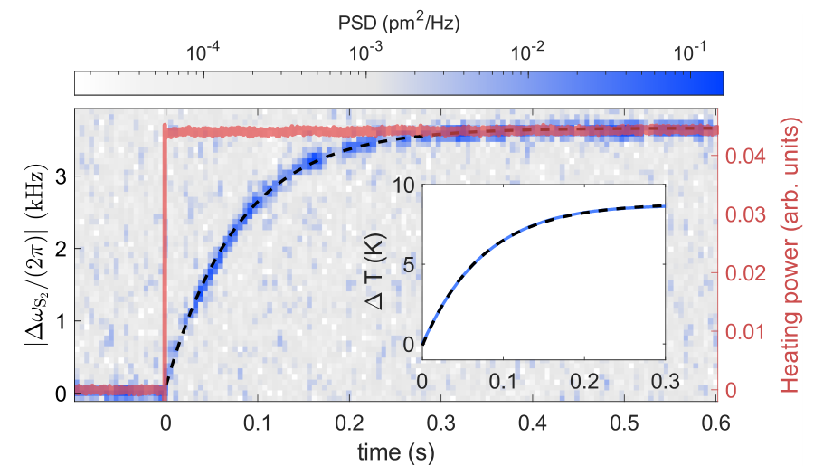
Next, we turn to using these results and obtain the spatial temperature distribution across our resonator. A full description of the steady state temperature map of the heat equation requires knowledge of the thermal conductivity $k_{c}$, emissivity $\varepsilon$ and heat load $P_{\mathrm{heat}}$. Measuring both $\tilde{T}^{\left(\mathrm{S}_{2}\right)}_{\mathrm{eff}}$ and $\tilde{T}^{\left(\mathrm{MD}\right)}_{\mathrm{eff}}$ provides the physical temperatures $T_{\mathrm{cp}}$ and $T_{\mathrm{ab}}$ respectively. These two independent measurements are insufficient to fully constrain the three parameters of the heat equation. A measurement of the thermalization time scale $\tau_{\mathrm{th}}$ provides additional knowledge about $k_{c}$ and $\varepsilon$ independent of $P_{\mathrm{heat}}$. Fig. 3 shows the $\mathrm{S}_{2}$ mode frequency shift $\Delta\omega_{\mathrm{S}_{2}}$ when the absorber is subjected to a step heat load. The frequencies quasistatically follow the instantaneous temperature profile of the device, and thus the timescale of the frequency change is equal to $\tau_{\mathrm{th}}$. Fitting the result to an FEA simulation of the time dependent temperature profile allows for a necessary constraint $k_{c}(\varepsilon)$ needed to explain the value of $1/\tau_{\mathrm{th}}$ = 12.5 Hz (inset Fig. 3). This knowledge in addition to the aforementioned two independent local temperature measurements generates the temperature map across our resonator for various heating powers. Once the temperature maps are known, FEA simulations of the normal mode frequencies can be matched to experiment for a determination of the coefficient of thermal expansion as well (detailed calculation of the temperature map along with an example of measurement-based FEA temperature map are given in Appendix A).

The effective temperature of the modes chosen for our analysis thus far was essentially affected by a single physical temperature - the local temperature at the location of their confined dissipation density (Fig. 1 and Fig. 2(b). As a simplest further study, we examined the case in which a single mode is influenced by two different local temperatures, which was made possible owing to the non-uniform local temperature.

When a mechanical resonator is held at a uniform temperature, a change in that temperature would lead to identical relative frequency shift for all the modes, meaning $\frac{\Delta f_{i}}{f_{i}}$ is identical for any mode $i$, where $\Delta f_{i}$ is the change of frequency $f_{i}$ due to the temperature change. In this case, two modes would never cross in frequency. However, non-uniform heating generates non-uniform thermal stress change, such that the fractional frequency shift differs between modes Jöckel et al. 2011; St-Gelais et al. 2019; Sadeghi et al. 2020, and they may cross in frequency. Indeed, in our device, for some absorber heating the $\mathrm{MD}$ and $\mathrm{S}_{2}$ fractional shifts satisfy $\frac{\Delta f_{\mathrm{MD}}}{f_{\mathrm{MD}}}\approx 13\>\frac{\Delta f_{\mathrm{S}_{2}}}{f_{\mathrm{S}_{2}}}$.

This allows us to examine the hybridization of these two in-bandgap modes, as a mode coupled to two thermal baths. As shown above, these two modes dissipation densities are restricted to different regions of the resonator, held at different local temperature when the absorber is heated. The frequencies of the $\mathrm{S}_{2}$ and $\mathrm{MD}$ modes for different heating power are shown in Fig. 4(a). The $\mathrm{S}_{2}$ and the $\mathrm{MD}$ frequencies were fitted and extrapolated with linear and quadratic polynomials, respectively. The quadratic polynomial was used because of a mode at $2.465\>\mathrm{MHz}$, with which the $\mathrm{MD}$ mode hybridized, making the $\mathrm{MD}$ frequency shift non linear. The hybridization gap of $\approx 500\>\mathrm{Hz}$ (on par with similar related studies Catalini et al. 2020) between the symmetric and antisymmetric branches (inset in Fig. 4(a)) and the associated mode shapes were estimated from an FEA calculation.

As a result of the hybridization, each of two modes in the pair changes its effective mass. Inference of effective temperature from displacement power should, in principle, take this change into account. This requires precise modeling and stable heating, which is challenging. To circumvent these requirements, we examine the quantity

which is defined with respect to the center pad motion. In words, $y_{\left(\mathrm{S}_{2},\mathrm{MD}\right)}^{2}$ is the total displacement power of the resonator middle pad at both modes’ frequencies. Furthermore, we can define the parameter

which has units of temperature and is defined similarly to the definition in Eq. 3. Here, $\omega_{\mathrm{S}_{2}}$ is the extrapolated angular frequency of the $\mathrm{S}_{2}$ mode without hybridization. As it turns out, this temperature does not depend on the effective mass changes due to the mode coupling, yet can still carry information about the local temperatures of the two non-hybridized modes. A detailed derivation of $\tilde{\mathcal{T}}^{\left(\mathrm{S}_{2},\mathrm{MD}\right)}_{\mathrm{eff}}$ is given in Appendix B. In general, it depends on the dissipation, the effective mass, the frequency, and the coupling between the two modes, as well as the local bath temperature of each mode, namely $T_{\mathrm{cp}}$ and $T_{\mathrm{ab}}$. It is, however, constructive to write the expected value for $\tilde{\mathcal{T}}^{\left(\mathrm{S}_{2},\mathrm{MD}\right)}_{\mathrm{eff}}$ in two specific limits:

Fig. 4(b) shows $\tilde{\mathcal{T}}^{\left(\mathrm{S}_{2},\mathrm{MD}\right)}_{\mathrm{eff}}$ as a function of $\Delta f_{1,1}$. The line is a single parameter fit, taking only the measurements around $\Delta f_{1,1}=0$ and $\Delta_{1,1}\approx 1.2\>\mathrm{kHz}$, which are far detuned from the point of hybridization. This line, which agrees with the linear fit in Fig. 2(b), stands for $T_{\mathrm{cp}}$ inferred from $y_{\left(\mathrm{S}_{2},\mathrm{MD}\right)}^{2}$. According to Eq. 6, a deviation from this line necessarily means that $T_{\mathrm{cp}}\neq T_{\mathrm{sb}}$, meaning that a single hybridized mode is affected by two different thermal baths. The height of the peak around $\Delta f_{1,1}$ is lower than expected value of $750\mathrm{K}$ according to the second limit in Eq. 6 (Appendix B). We believe this is due to heating power fluctuations, originating primarily from motion of the heating beam and temporal changes absorber heating (see Appendix D).

To conclude, in this work we designed and implemented a controlled local temperature measurement of a SiN resonator under localized heating, by measuring the Brownian motion of a set of localized normal modes. We experimentally demonstrated that in the presence of a non-uniform temperature profile, different modes might have exceedingly different effective temperatures, depending on the spatial overlap between the local temperature and the dissipation density of a mode. This demonstration was done both by measuring the Brownian motion of different modes and by in-situ hybridization of two modes with different local baths. We compared between a membrane-like mode, having effective temperature identical to the resonator’s environment with the price of higher dissipation at its edge, to a localized mode, potentially designed for lower dissipation, with the price of an effective temperature equal to the local — typically hotter — temperature at the mode’s confined location. These represent two extreme scenarios of susceptibility to uneven heating. A resonator’s optimal performance would be achieved when its design minimizes the overlap between the dissipation density and the local temperature profile.

$*$ R.S and C.R contributed equally to this work.

References

- Passaro et al. (2017) V. M. Passaro, A. Cuccovillo, L. Vaiani, M. De Carlo, and C. E. Campanella, Sensors 17, 2284 (2017).
- Krause et al. (2012) A. G. Krause, M. Winger, T. D. Blasius, Q. Lin, and O. Painter, Nature Photonics 6, 768 (2012).
- Giessibl (2003) F. J. Giessibl, Reviews of modern physics 75, 949 (2003).
- Poggio and Degen (2010) M. Poggio and C. L. Degen, Nanotechnology 21, 342001 (2010).
- Degen et al. (2009) C. Degen, M. Poggio, H. Mamin, C. Rettner, and D. Rugar, Proceedings of the National Academy of Sciences 106, 1313 (2009).
- Arlett et al. (2011) J. Arlett, E. Myers, and M. Roukes, Nature nanotechnology 6, 203 (2011).
- Bleszynski-Jayich et al. (2009) A. Bleszynski-Jayich, W. Shanks, B. Peaudecerf, E. Ginossar, F. Von Oppen, L. Glazman, and J. Harris, Science 326, 272 (2009).
- Andrews et al. (2014) R. W. Andrews, R. W. Peterson, T. P. Purdy, K. Cicak, R. W. Simmonds, C. A. Regal, and K. W. Lehnert, Nature Physics 10, 321 (2014).
- Wallucks et al. (2020) A. Wallucks, I. Marinković, B. Hensen, R. Stockill, and S. Gröblacher, Nature Physics 16, 772 (2020).
- Barzanjeh et al. (2022) S. Barzanjeh, A. Xuereb, S. Gröblacher, M. Paternostro, C. A. Regal, and E. M. Weig, Nature Physics 18, 15 (2022).
- Schmöle et al. (2016) J. Schmöle, M. Dragosits, H. Hepach, and M. Aspelmeyer, Classical and Quantum Gravity 33, 125031 (2016).
- Liu et al. (2021) Y. Liu, J. Mummery, J. Zhou, and M. A. Sillanpää, Physical Review Applied 15, 034004 (2021).
- Carney et al. (2021) D. Carney, G. Krnjaic, D. C. Moore, C. A. Regal, G. Afek, S. Bhave, B. Brubaker, T. Corbitt, J. Cripe, N. Crisosto, et al., Quantum Science and Technology 6, 024002 (2021).
- Piller et al. (2022) M. Piller, J. Hiesberger, E. Wistrela, P. Martini, N. Luhmann, and S. Schmid, IEEE Sensors Journal (2022).
- Harry et al. (2010) G. M. Harry, for the LIGO Scientific Collaboration, et al., Classical and Quantum Gravity 27, 084006 (2010).
- Riedinger et al. (2018) R. Riedinger, A. Wallucks, I. Marinković, C. Löschnauer, M. Aspelmeyer, S. Hong, and S. Gröblacher, Nature 556, 473 (2018).
- Mirhosseini et al. (2020) M. Mirhosseini, A. Sipahigil, M. Kalaee, and O. Painter, Nature 588, 599 (2020).
- Qiu et al. (2020) L. Qiu, I. Shomroni, P. Seidler, and T. J. Kippenberg, Physical Review Letters 124, 173601 (2020).
- Peterson et al. (2016) R. Peterson, T. Purdy, N. Kampel, R. Andrews, P.-L. Yu, K. Lehnert, and C. Regal, Physical review letters 116, 063601 (2016).
- Page et al. (2021) M. A. Page, M. Goryachev, H. Miao, Y. Chen, Y. Ma, D. Mason, M. Rossi, C. D. Blair, L. Ju, D. G. Blair, et al., Communications Physics 4, 27 (2021).
- Lax (1960) M. Lax, Reviews of modern physics 32, 25 (1960).
- Komori et al. (2018) K. Komori, Y. Enomoto, H. Takeda, Y. Michimura, K. Somiya, M. Ando, and S. W. Ballmer, Physical Review D 97, 102001 (2018).
- Geitner et al. (2017) M. Geitner, F. A. Sandoval, E. Bertin, and L. Bellon, Physical Review E 95, 032138 (2017).
- Singh and Purdy (2020) R. Singh and T. P. Purdy, Physical Review Letters 125, 120603 (2020).
- Ghadimi et al. (2018) A. H. Ghadimi, S. A. Fedorov, N. J. Engelsen, M. J. Bereyhi, R. Schilling, D. J. Wilson, and T. J. Kippenberg, Science 360, 764 (2018).
- Fedorov et al. (2020) S. A. Fedorov, A. Beccari, N. J. Engelsen, and T. J. Kippenberg, Physical Review Letters 124, 025502 (2020).
- Høj et al. (2021) D. Høj, F. Wang, W. Gao, U. B. Hoff, O. Sigmund, and U. L. Andersen, Nature communications 12, 5766 (2021).
- Bereyhi et al. (2022) M. J. Bereyhi, A. Arabmoheghi, A. Beccari, S. A. Fedorov, G. Huang, T. J. Kippenberg, and N. J. Engelsen, Physical Review X 12, 021036 (2022).
- Pluchar et al. (2022) C. M. Pluchar, A. R. Agrawal, C. A. Condos, J. Pratt, S. Schlamminger, and D. Wilson, in Optical Trapping and Optical Micromanipulation XIX (SPIE, 2022) p. PC121980U.
- Eichenfield et al. (2009) M. Eichenfield, J. Chan, R. M. Camacho, K. J. Vahala, and O. Painter, nature 462, 78 (2009).
- Clerk et al. (2010) A. A. Clerk, M. H. Devoret, S. M. Girvin, F. Marquardt, and R. J. Schoelkopf, Reviews of Modern Physics 82, 1155 (2010).
- Kushwaha et al. (1993) M. S. Kushwaha, P. Halevi, L. Dobrzynski, and B. Djafari-Rouhani, Physical review letters 71, 2022 (1993).
- Tsaturyan et al. (2017) Y. Tsaturyan, A. Barg, E. S. Polzik, and A. Schliesser, Nature nanotechnology 12, 776 (2017).
- Zhang et al. (2020) C. Zhang, M. Giroux, T. A. Nour, and R. St-Gelais, Physical Review Applied 14, 024072 (2020).
- Leivo and Pekola (1998) M. Leivo and J. Pekola, Applied Physics Letters 72, 1305 (1998).
- Vicarelli et al. (2022) L. Vicarelli, A. Tredicucci, and A. Pitanti, ACS photonics 9, 360 (2022).
- Piller et al. (2020) M. Piller, P. Sadeghi, R. G. West, N. Luhmann, P. Martini, O. Hansen, and S. Schmid, Applied Physics Letters 117, 034101 (2020).
- Reetz et al. (2019) C. Reetz, R. Fischer, G. G. Assumpcao, D. P. McNally, P. S. Burns, J. C. Sankey, and C. A. Regal, Physical Review Applied 12, 044027 (2019).
- Turner et al. (2001) A. D. Turner, J. J. Bock, J. W. Beeman, J. Glenn, P. C. Hargrave, V. V. Hristov, H. T. Nguyen, F. Rahman, S. Sethuraman, and A. L. Woodcraft, Applied Optics 40, 4921 (2001).
- Høj et al. (2022) D. Høj, U. B. Hoff, and U. L. Andersen, arXiv preprint arXiv:2207.06703 (2022).
- Jöckel et al. (2011) A. Jöckel, M. T. Rakher, M. Korppi, S. Camerer, D. Hunger, M. Mader, and P. Treutlein, Applied physics letters 99, 143109 (2011).
- St-Gelais et al. (2019) R. St-Gelais, S. Bernard, C. Reinhardt, and J. C. Sankey, ACS Photonics 6, 525 (2019).
- Sadeghi et al. (2020) P. Sadeghi, M. Tanzer, N. Luhmann, M. Piller, M.-H. Chien, and S. Schmid, Physical Review Applied 14, 024068 (2020).
- Catalini et al. (2020) L. Catalini, Y. Tsaturyan, and A. Schliesser, Physical Review Applied 14, 014041 (2020).