跳到论文正文
W Papers独立论文阅读器 arXiv:2305.05277 论文正文 计算阅读时间 · 0%
引用这篇论文根据当前论文元数据生成,正式投稿前建议核对。


License: arXiv.org perpetual non-exclusive license
arXiv:2305.05277v2 [cs.IT] 10 May 2023

Dept. of ECE, The Hong Kong University of Science and Technology, Hong Kong

Active IRS-Aided MIMO Systems: How Much Gain Can We Get?

Zeyan Zhuang, Xin Zhang, Dongfang Xu, and Shenghui Song
Abstract

Intelligent reflecting surfaces (IRSs) have emerged as a promising technology to improve the efficiency of wireless communication systems. However, passive IRSs suffer from the “multiplicative fading” effect, because the transmit signal will go through two fading hops. With the ability to amplify and reflect signals, active IRSs offer a potential way to tackle this issue, where the amplification energy only experiences the second hop. However, the fundamental limit and system design for active IRSs have not been fully understood, especially for multiple-input multiple-output (MIMO) systems. In this work, we consider the analysis and design for the large-scale active IRS-aided MIMO system assuming only statistical channel state information (CSI) at the transmitter and the IRS. The evaluation of the fundamental limit, i.e., ergodic rate, turns out to be a very difficult problem. To this end, we leverage random matrix theory (RMT) to derive the deterministic approximation (DA) for the ergodic rate, and then design an algorithm to jointly optimize the transmit covariance matrix at the transmitter and the reflection matrix at the active IRS. Numerical results demonstrate the accuracy of the derived DA and the effectiveness of the proposed optimization algorithm. The results in this work reveal interesting physical insights with respect to the advantage of active IRSs over their passive counterparts.

I Introduction

With the development of innovative applications, there is an increasing demand for higher data rate, reliability, and energy efficiency in future wireless communication systems. To this end, intelligent reflecting surfaces (IRSs), have been proposed as an energy-efficient way to create a favorable channel between the transmitter and receiver [1, 2]. Specifically, IRSs can reshape the wireless channel and improve the signal quality by reflecting signals through a surface composed of a large number of reconfigurable elements.

Many engaging results have been obtained on the analysis and design of IRS-aided systems such as the IRS-aided multiple-input single-output (MISO) [1] and multiple-input multiple-output (MIMO) channels [3, 4, 5]. In particular, [3] studied the fundamental limit of IRS-aided point-to-point MIMO systems with perfect channel state information (CSI) at the transmitter, receiver, and IRS. However, in practice, perfect CSI is extremely difficult to obtain for IRS-aided systems, especially in the case of fast-fading channels [6]. As a result, [4] investigated the achievable rate of a large-scale passive IRS-aided MIMO system where only statistical CSI is available at the transmitter and the IRS, by random matrix theory (RMT). The design of the transmit covariance matrix and the phase-shift matrix was also considered.

With either perfect or statistical CSI, the potential gain brought by IRSs is often limited by the “multiplicative fading” of the two-hop channel [7]. To circumvent this issue, a new IRS architecture, namely, active IRS, has recently been proposed in [8]. In particular, equipped with the reflection-type amplifiers (e.g., current-inverting converters), active IRSs can not only reflect the signal to a desired direction, but also amplify the signal with additional power [9]. It is worth mentioning that active IRSs and full-duplex (FD) amplify-and-forward (AF) relays differ in both hardware implementation and transmission modes [1]. Specifically, FD AF relays lead to unavoidable self-interference and processing delay when amplifying the received signal. In contrast, active IRSs can amplify signals instantaneously without introducing self-interference, although the processing freedom is limited, i.e., the diagonal reflection matrix. Inspired by these advantages, some researchers have investigated the analysis and design of active IRS-aided systems. In particular, [10, 9] compared the performance of active and passive IRS-aided single-input single-output (SISO) systems given the same overall power budget. The authors of [11] investigated the fundamental limits of IRS-aided MISO systems with partial CSI. However, to the best of the authors’ knowledge, the fundamental limits of active IRS-aided MIMO systems are not yet available in the literature.

Motivated by the above works, in this paper, we investigate the active IRS-aided point-to-point MIMO communication system assuming only statistical CSI at the transmitter and the IRS. The objective is to first determine the fundamental limit of the concerned system, i.e., the ergodic rate. Then, based on the evaluation result, we jointly design the transmit covariance matrix and the reflection matrix to maximize the ergodic rate. We achieve the first objective by deriving the deterministic approximation (DA) of the ergodic rate using RMT. As the optimization problem is non-convex, we propose an alternating optimization (AO)-based algorithm to design the optimal transmit covariance matrix and reflection matrix. Numerical results validate the accuracy of the DA and effectiveness of the proposed algorithm.

The main contributions of this work include:

  • •

    We evaluate the ergodic rate of active IRS-aided MIMO systems with only statistical CSI at the transmitter and the IRS. To obtain a more tractable and computationally-efficient form for ease of use in the following optimization, we derive the DA for the ergodic rate.

  • •

    We maximize the DA for the ergodic rate by jointly optimizing the transmit covariance matrix and reflection matrix. To tackle the resulting non-convex optimization problem, an AO-based low-complexity suboptimal algorithm is developed.

  • •

    We investigate the impact of the dynamic noise introduced by the active IRS and different power allocation policies. Simulation results unveil that the active IRS is effective to tackle the “multiplicative fading” effect and has consistent advantages over the passive one.

The rest of this paper is organized as follows. In section II, we introduce the system model and formulate the problem. In section III, we derive the DA for the ergodic rate. An AO-based algorithm for optimizing the transmit covariance matrix and the reflection matrix is proposed in section IV. Section V gives the numerical results and Section VI concludes the paper. The notations utilized in this paper are listed in the footnote11 1 Notations. In this paper, we use boldfaced uppercase letters and lowercase letters to represent matrices and column vectors, respectively. ℑ⁡(a)\Im(a) and ℜ⁡(a)\Re(a) denote the imaginary and real part of a complex number aa, respectively. ℝ+\mathbb{R}^{+} and ℂ+\mathbb{C}^{+} denote the real non-negative axis {x∈ℝ:x≥0}\{x\in\mathbb{R}:x\geq 0\} and the upper half plane {z∈ℂ:ℑ⁡(z)>0}\{z\in\mathbb{C}:\Im(z)>0\}, respectively. Let ȷ=−1\jmath=\sqrt{-1}. The (i,j)(i,j)-th element of matrix 𝐀\mathbf{A} will be denoted as either ai​ja_{ij} or [𝐀]i​j[\mathbf{A}]_{ij}. diag​{𝐚}\mathrm{diag}\{\mathbf{a}\} denotes the diagonal square matrix whose diagonal entries are elements of vector 𝐚\mathbf{a} and diag{𝐀}=diag{ai​i;1≤i≤n}\mathrm{diag}\{\mathbf{A}\}=\mathrm{diag}\{a_{ii};1\leq i\leq n\} for all n×nn\times n matrix 𝐀\mathbf{A}. The superscript ‘HH’ denotes Hermitian transpose operator. Tr⁡(𝐀)\mathrm{Tr}(\mathbf{A}) and ‖𝐀‖||\mathbf{A}|| represent the trace and spectral norm of 𝐀\mathbf{A}, respectively. 𝔼⁡[a]\mathbb{E}[a] denotes the expectation of random variable aa. Function (a)+=max⁡{a,0}(a)^{+}=\max\{a,0\}. →Xa.s.\xrightarrow[\mathrm{X}]{a.s.} represents the almost sure convergence under the process X. supp⁡(μ)\mathrm{supp}(\mu) denotes the support of measure μ\mu..

Refer to caption
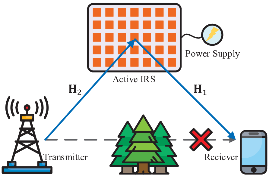
Fig. 1: Active IRS-aided communication system.

II System model and Problem Formulation

II-A System Model

As shown in Fig. 1, we consider a MIMO system consisting of a base station (BS) equipped with ntn_{t} transmit antennas and a user equipped with nrn_{r} receive antennas. Due to the blockage of the direct link, an IRS comprising nln_{l} active reflecting elements is utilized to establish an alternative communication link. Due to the active nature, the thermal noise introduced during amplification cannot be ignored [8]. Therefore, the received signal 𝐲\mathbf{y} at the user side is given by

𝐲=𝐇1​𝚽​𝐇2​𝐱+𝐇1​𝚽​𝐧d+𝐧s,\displaystyle\mathbf{y}=\mathbf{H}_{1}\mathbf{\Phi}\mathbf{H}_{2}\mathbf{x}+\mathbf{H}_{1}\mathbf{\Phi}\mathbf{n}_{d}+\mathbf{n}_{s}, (1)

where 𝐱∈ℂnt\mathbf{x}\in\mathbb{C}^{n_{t}} denotes the transmit signal with covariance matrix 𝐐=𝔼⁡[𝐱𝐱H]\mathbf{Q}=\mathbb{E}[\mathbf{x}\mathbf{x}^{H}]. The matrices 𝐇2∈ℂnl×nt\mathbf{H}_{2}\in\mathbb{C}^{n_{l}\times n_{t}}, 𝐇1∈ℂnr×nl\mathbf{H}_{1}\in\mathbb{C}^{n_{r}\times n_{l}} represent BS-IRS and IRS-user channel, respectively. The reflection matrix of the active IRS is denoted by 𝚽=diag⁡{a1​ϕ1,a2​ϕ2,⋯,anl​ϕnl}\mathbf{\Phi}=\mathrm{diag}\{a_{1}\phi_{1},a_{2}\phi_{2},\cdots,a_{n_{l}}\phi_{n_{l}}\}, where ai∈ℝ+a_{i}\in\mathbb{R^{+}} and ϕi=eȷ​θi\phi_{i}=e^{\jmath\theta_{i}}, i=1,2,⋯,nli=1,2,\cdots,n_{l} represent the amplification factor and phase shift of the ii-th IRS element, respectively. Different from the passive IRS, aia_{i} can be larger than 11. Here 𝐧d∈ℂnl\mathbf{n}_{d}\in\mathbb{C}^{n_{l}} denotes the dynamic noise introduced by the active component and 𝐧s∈ℂnr\mathbf{n}_{s}\in\mathbb{C}^{n_{r}} is the static noise at the receiver. Both 𝐧d\mathbf{n}_{d} and 𝐧s\mathbf{n}_{s} are modeled as additive Gaussian white noise (AWGN)[8] [12], i.e., 𝐧d∼𝒞​𝒩​(𝟎,σd2​𝐈)\mathbf{n}_{d}\sim\mathcal{CN}(\mathbf{0},\sigma_{d}^{2}\mathbf{I}), 𝐧s∼𝒞​𝒩​(𝟎,σs2​𝐈)\mathbf{n}_{s}\sim\mathcal{CN}(\mathbf{0},\sigma_{s}^{2}\mathbf{I}).

Assuming only statistical CSI at the transmitter and the IRS, the normalized ergodic rate of the channel is given by

R⁡(𝐐,𝚽)\displaystyle R(\mathbf{Q},\mathbf{\Phi})\hskip-5.69054pt =\displaystyle= 1nr𝔼[logdet(1σs2𝐇1𝚽𝐇2𝐐𝐇2H𝚽H𝐇1H+σd2σs2𝐇1𝚽𝚽H𝐇1H+𝐈)\displaystyle\hskip-5.69054pt\frac{1}{n_{r}}\mathbb{E}\Big[\log\det\big(\frac{1}{\sigma_{s}^{2}}\mathbf{H}_{1}\mathbf{\Phi}\mathbf{H}_{2}\mathbf{Q}\mathbf{H}_{2}^{H}\mathbf{\Phi}^{H}\mathbf{H}_{1}^{H}+\frac{\sigma_{d}^{2}}{\sigma_{s}^{2}}\mathbf{H}_{1}\mathbf{\Phi}\mathbf{\Phi}^{H}\mathbf{H}_{1}^{H}+\mathbf{I}\big) (2)
−\displaystyle- logdet(σd2σs2𝐇1𝚽𝚽H𝐇1H+𝐈)],\displaystyle\hskip-5.69054pt\log\det\big(\frac{\sigma_{d}^{2}}{\sigma_{s}^{2}}\mathbf{H}_{1}\mathbf{\Phi}\mathbf{\Phi}^{H}\mathbf{H}_{1}^{H}+\mathbf{I}\big)\Big],

where R⁡(𝐐,𝚽)R(\mathbf{Q},\mathbf{\Phi}) has the unit of bits per second per Hz per antenna. The channel matrix can be written by the Kronecker model as

𝐇1=𝐑112​𝐗1​𝐓112​ and ​𝐇2=𝐑212​𝐗2​𝐓212,\displaystyle\mathbf{H}_{1}=\mathbf{R}_{1}^{\frac{1}{2}}\mathbf{X}_{1}\mathbf{T}_{1}^{\frac{1}{2}}\mbox{ and }\mathbf{H}_{2}=\mathbf{R}_{2}^{\frac{1}{2}}\mathbf{X}_{2}\mathbf{T}_{2}^{\frac{1}{2}}, (3)

where 𝐑1∈ℂnr×nr\mathbf{R}_{1}\in\mathbb{C}^{n_{r}\times n_{r}}, 𝐓1∈ℂnl×nl\mathbf{T}_{1}\in\mathbb{C}^{n_{l}\times n_{l}} , 𝐑2∈ℂnl×nl\mathbf{R}_{2}\in\mathbb{C}^{n_{l}\times n_{l}} and 𝐓2∈ℂnt×nt\mathbf{T}_{2}\in\mathbb{C}^{n_{t}\times n_{t}} are Hermitian non-negative definite matrices. 𝐑1\mathbf{R}_{1} and 𝐓2\mathbf{T}_{2} represent the spatial correlation matrices for the receiver and the transmitter, while 𝐑2\mathbf{R}_{2} and 𝐓1\mathbf{T}_{1} denote the spatial correlation matrices for the IRS. We utilize L1L_{1} and L2L_{2} to denote the path loss for the IRS-user and BS-IRS link, respectively. For ease of manipulation, LiL_{i} is absorbed into 𝐑i\mathbf{R}_{i}. 𝐗1=ℂnr×nl\mathbf{X}_{1}=\mathbb{C}^{n_{r}\times n_{l}} and 𝐗2∈ℂnl×nt\mathbf{X}_{2}\in\mathbb{C}^{n_{l}\times n_{t}} are matrices whose entries are independent and identically distributed (i.i.d.) Gaussian random variables (r.v.s) with [𝐗1]i​j∼𝒞​𝒩​(0,1nl)[\mathbf{X}_{1}]_{ij}\sim\mathcal{CN}(0,\frac{1}{n_{l}}), [𝐗2]i​j∼𝒞​𝒩​(0,1nt)[\mathbf{X}_{2}]_{ij}\sim\mathcal{CN}(0,\frac{1}{n_{t}}). For simplicity, we define

𝐓~1=𝚽H​𝐓1​𝚽​ and ​𝐓~2=𝐐12​𝐓2​𝐐12.\widetilde{\mathbf{T}}_{1}=\mathbf{\Phi}^{H}\mathbf{T}_{1}\mathbf{\Phi}\mbox{ and }\widetilde{\mathbf{T}}_{2}=\mathbf{Q}^{\frac{1}{2}}\mathbf{T}_{2}\mathbf{Q}^{\frac{1}{2}}. (4)

Due to the rotational invariance of Gaussian distribution, the normalized ergodic rate can be written as

R(𝐐,𝚽)=1nr𝔼[logdet(𝐁1σs2+𝐈)−logdet(𝐁2σs2+𝐈)],R(\mathbf{Q},\mathbf{\Phi})=\frac{1}{n_{r}}\mathbb{E}\big[\log\det\big(\frac{\mathbf{B}_{1}}{\sigma_{s}^{2}}+\mathbf{I}\big)-\log\det\big(\frac{\mathbf{B}_{2}}{\sigma_{s}^{2}}+\mathbf{I}\big)\big], (5)

where 𝐁1=(𝐇~1​𝐇~2​𝐇~2H​𝐇~1H+σd2​𝐇~1​𝐇~1H)\mathbf{B}_{1}=(\widetilde{\mathbf{H}}_{1}\widetilde{\mathbf{H}}_{2}\widetilde{\mathbf{H}}_{2}^{H}\widetilde{\mathbf{H}}_{1}^{H}+\sigma_{d}^{2}\widetilde{\mathbf{H}}_{1}\widetilde{\mathbf{H}}_{1}^{H}), 𝐁2=σd2​𝐇~1​𝐇~1H\mathbf{B}_{2}=\sigma_{d}^{2}\widetilde{\mathbf{H}}_{1}\widetilde{\mathbf{H}}_{1}^{H}, 𝐇~1=𝐑112​𝐗1​𝐓~112\widetilde{\mathbf{H}}_{1}=\mathbf{R}_{1}^{\frac{1}{2}}\mathbf{X}_{1}\widetilde{\mathbf{T}}_{1}^{\frac{1}{2}}, and 𝐇~2=𝐑212​𝐗2​𝐓~212\widetilde{\mathbf{H}}_{2}=\mathbf{R}_{2}^{\frac{1}{2}}\mathbf{X}_{2}\widetilde{\mathbf{T}}_{2}^{\frac{1}{2}}.

II-B Problem Formulation

Our objective is to optimize the normalized ergodic rate of the active IRS-aided MIMO system under the power constraint at both the transmitter and IRS. The problem can be formulated as

𝒫1:\displaystyle\mathcal{P}_{1}: maximize𝐐⪰𝟎,𝚽​R​(𝐐,𝚽)\displaystyle\underset{\mathbf{Q}\succeq\mathbf{0},\bm{\Phi}}{\maxo}\hskip 5.69054ptR(\mathbf{Q},\bm{\Phi}) (6)
s.t.C1:Tr(𝐐)≤ntPT,\displaystyle\hskip 14.22636pt\mbox{s.t.}\hskip 19.91692pt\mbox{C1:}\hskip 2.84526pt\mathrm{Tr}(\mathbf{Q})\leq n_{t}P_{T},
C2:Tr⁡(𝐐𝐓2)ntTr(𝐑2(𝚽𝚽H−𝐈))+σd2Tr(𝚽𝚽H)≤PA,\displaystyle\hskip 48.36967pt\mbox{C2:}\hskip 2.84526pt\frac{\mathrm{Tr}(\mathbf{Q}\mathbf{T}_{2})}{n_{t}}\mathrm{Tr}(\mathbf{R}_{2}(\mathbf{\Phi}\mathbf{\Phi}^{H}-\mathbf{I}))+\sigma_{d}^{2}\mathrm{Tr}(\mathbf{\Phi}\mathbf{\Phi}^{H})\leq P_{A},

where C1 represents the maximum power constraint at the transmitter and C2 denotes the amplification power budget of the active IRS.

Remark 1.

The received signal of the active IRS is 𝐬i​n=𝐇2​𝐱\mathbf{s}_{in}=\mathbf{H}_{2}\mathbf{x} and the reflected signal is 𝐬o​u​t=𝚽​𝐇2​𝐱+𝚽​𝐧d\mathbf{s}_{out}=\mathbf{\Phi}\mathbf{H}_{2}\mathbf{x}+\mathbf{\Phi}\mathbf{n}_{d}. The amplification power of the active IRS is 𝔼⁡[𝐬o​u​tH​𝐬o​u​t]\mathbb{E}[\mathbf{s}_{out}^{H}\mathbf{s}_{out}] [8, 1]. However, if we set the power constraint as 𝔼⁡[𝐬o​u​tH​𝐬o​u​t]≤PA\mathbb{E}[\mathbf{s}_{out}^{H}\mathbf{s}_{out}]\leq P_{A}, then when PA→0P_{A}\rightarrow 0, i.e., there is no power supply at IRS, the amplification factor aia_{i} will become 00. To ensure a fair comparison with the passive IRS, we subtract the received energy of the IRS from the amplification energy and formulate the constraint as in C2. Therefore, the total power consumed by the active IRS is 𝔼⁡[𝐬o​u​tH​𝐬o​u​t]−𝔼⁡[𝐬i​nH​𝐬i​n]\mathbb{E}[\mathbf{s}_{out}^{H}\mathbf{s}_{out}]-\mathbb{E}[\mathbf{s}_{in}^{H}\mathbf{s}_{in}].

Note that 𝒫1\mathcal{P}_{1} is very challenging to solve for two reasons. Firstly, the objective function is the expectation over a log determinant. Secondly, the objective function is the difference between two terms and the constraints C1 and C2 are coupled, making the optimization problem non-convex. In the following, we first derive the DA to approximate the normalized ergodic rate and then propose an effective AO-based algorithm to jointly optimize the transmit covariance matrix and the reflection matrix.

III Deterministic Approximation of Ergodic Rate

Direct evaluation of the ergodic rate is very difficult. In this section, we first derive the DA for the normalized ergodic rate by leveraging RMT. For that purpose, we first introduce two important assumptions.

Assumption A-1.

Let c1=nrnlc_{1}=\frac{n_{r}}{n_{l}}, c2=nlntc_{2}=\frac{n_{l}}{n_{t}}, then 0<liminf⁡c1≤limsup⁡c1<+∞0<\lim\inf c_{1}\leq\lim\sup c_{1}<+\infty, 0<liminf⁡c2≤limsup⁡c2<+∞0<\lim\inf c_{2}\leq\lim\sup c_{2}<+\infty.

Assumption A-2.

lim supn¯→+∞​(maxi=1,2​{‖𝐑i‖,‖𝐓~i‖})<+∞\underset{\overline{n}\rightarrow+\infty}{\limsup}\hskip 2.84526pt(\underset{i=1,2}{\max}\{||\mathbf{R}_{i}||,\hskip 2.84526pt||\widetilde{\mathbf{T}}_{i}||\})<+\infty.

A-1 implies that the number of transmit antennas, receive antennas, and active IRS elements grow to +∞+\infty at the same rate. In the following, we use n¯→+∞\overline{n}\rightarrow+\infty to represent this asymptotic regime. A-2 implies that the antenna imbalance is finite [13].

For a positive measure μ\mu over ℝ\mathbb{R}, its Stieltjes transform is defined as mμ​(z)=∫ℝμ⁡(d​t)t−z,z∈ℂ\supp⁡(μ)m_{\mu}(z)=\int_{\mathbb{R}}\frac{\mu(\mathrm{d}t)}{t-z},z\in\mathbb{C}\backslash\mathrm{supp}(\mu). We denote 𝒮⁡(𝔻)\mathcal{S}(\mathbb{D}) as the set of Stieltjes transforms for positive measures over domain 𝔻\mathbb{D}. For matrix 𝐌∈ℂn×n\mathbf{M}\in\mathbb{C}^{n\times n}, we denote 𝐐𝐌​(z)=(−z​𝐈+𝐌)−1\mathbf{Q}_{\mathbf{M}}(z)=(-z\mathbf{I}+\mathbf{M})^{-1} as its resolvent matrix and m𝐌​(z)=1n​Tr​𝐐𝐌​(z)m_{\mathbf{M}}(z)=\frac{1}{n}\mathrm{Tr}\mathbf{Q}_{\mathbf{M}}(z) represents the Stieltjes transform of its empirical spectrum distribution (ESD). In order to evaluate (5), we use the Shannon transform[14], i.e., R⁡(𝐐,𝚽)=∫σs2+∞𝔼⁡[m𝐁2​(−t)−m𝐁1​(−t)]​𝑑tR(\mathbf{Q},\bm{\Phi})=\int^{+\infty}_{\sigma_{s}^{2}}\mathbb{E}[m_{\mathbf{B}_{2}}(-t)-m_{\mathbf{B}_{1}}(-t)]\mathrm{d}t, where m𝐁1​(−t)m_{\mathbf{B}_{1}}(-t) and m𝐁2​(−t)m_{\mathbf{B}_{2}}(-t) are the Stieltjes transforms of the ESDs for 𝐁1\mathbf{B}_{1} and 𝐁2\mathbf{B}_{2} defined in (5). To approximate the ergodic rate, we first give the two DAs of 𝔼​[m𝐁1​(z)]\mathbb{E}[m_{\mathbf{B}_{1}}(z)] and 𝔼​[m𝐁2​(z)]\mathbb{E}[m_{\mathbf{B}_{2}}(z)] in the following two theorems.

Theorem 1.

With assumptions A-1 and A-2, we have

𝔼⁡[m𝐁1​(z)]−1nr​Tr​(−z​𝐈+(δ2​δ3+σd2​δ4)​𝐑1)−1→n¯→+∞0,\mathbb{E}[m_{\mathbf{B}_{1}}(z)]-\frac{1}{n_{r}}\mathrm{Tr}(-z\mathbf{I}+(\delta_{2}\delta_{3}+\sigma_{d}^{2}\delta_{4})\mathbf{R}_{1})^{-1}\xrightarrow{\overline{n}\rightarrow+\infty}0, (7)

where δi\delta_{i}, i=1,2,3,4i=1,2,3,4, is the unique solution of the following system of equations

δ1\displaystyle\delta_{1}\hskip-8.53581pt =\displaystyle= 1nr​Tr​[𝐑1​(−z​𝐈+(δ2​δ3+σd2​δ4)​𝐑1)−1],\displaystyle\hskip-8.53581pt\frac{1}{n_{r}}\mathrm{Tr}[\mathbf{R}_{1}(-z\mathbf{I}+(\delta_{2}\delta_{3}+\sigma_{d}^{2}\delta_{4})\mathbf{R}_{1})^{-1}], (8)
δ2\displaystyle\delta_{2}\hskip-8.53581pt =\displaystyle= 1nl​Tr​[𝐓~112​𝐑2​𝐓~112​(𝐈+σd2​c1​δ1​𝐓~1+c1​δ1​δ3​𝐓~112​𝐑2​𝐓~112)−1],\displaystyle\hskip-8.53581pt\frac{1}{n_{l}}\mathrm{Tr}[\widetilde{\mathbf{T}}_{1}^{\frac{1}{2}}\mathbf{R}_{2}\widetilde{\mathbf{T}}_{1}^{\frac{1}{2}}(\mathbf{I}\hskip-1.42262pt+\hskip-1.42262pt\sigma_{d}^{2}c_{1}\delta_{1}\widetilde{\mathbf{T}}_{1}\hskip-1.42262pt+\hskip-1.42262ptc_{1}\delta_{1}\delta_{3}\widetilde{\mathbf{T}}_{1}^{\frac{1}{2}}\mathbf{R}_{2}\widetilde{\mathbf{T}}_{1}^{\frac{1}{2}})^{-1}], (9)
δ3\displaystyle\delta_{3}\hskip-8.53581pt =\displaystyle= 1nt​Tr​[𝐓~2​(𝐈+c1​c2​δ1​δ2​𝐓~2)−1],\displaystyle\hskip-8.53581pt\frac{1}{n_{t}}\mathrm{Tr}[\widetilde{\mathbf{T}}_{2}(\mathbf{I}+c_{1}c_{2}\delta_{1}\delta_{2}\widetilde{\mathbf{T}}_{2})^{-1}], (10)
δ4\displaystyle\delta_{4}\hskip-8.53581pt =\displaystyle= 1nl​Tr​[𝐓~1​(𝐈+σd2​c1​δ1​𝐓~1+c1​δ1​δ3​𝐓~112​𝐑2​𝐓~112)−1],\displaystyle\hskip-8.53581pt\frac{1}{n_{l}}\mathrm{Tr}[\widetilde{\mathbf{T}}_{1}(\mathbf{I}+\sigma_{d}^{2}c_{1}\delta_{1}\widetilde{\mathbf{T}}_{1}+c_{1}\delta_{1}\delta_{3}\widetilde{\mathbf{T}}_{1}^{\frac{1}{2}}\mathbf{R}_{2}\widetilde{\mathbf{T}}_{1}^{\frac{1}{2}})^{-1}], (11)

such that {δ1,δ1​δ2,δ1​δ3,δ1​δ4}⊂𝒮⁡(ℝ+)\{\delta_{1},\delta_{1}\delta_{2},\delta_{1}\delta_{3},\delta_{1}\delta_{4}\}\subset\mathcal{S}(\mathbb{R}^{+}).

Proof: Please refer to Appendix A. ∎

Theorem 2.

With assumptions A-1 and A-2, we have

𝔼⁡[m𝐁2​(z)]−1nr​Tr​(−z​𝐈+α2​𝐑1)−1→n¯→+∞0,\mathbb{E}[m_{\mathbf{B}_{2}}(z)]-\frac{1}{n_{r}}\mathrm{Tr}(-z\mathbf{I}+\alpha_{2}\mathbf{R}_{1})^{-1}\xrightarrow{\overline{n}\rightarrow+\infty}0, (12)

where αi\alpha_{i}, i=1,2i=1,2, is the unique solution of the following system of equations

α1\displaystyle\alpha_{1}\hskip-8.53581pt =\displaystyle= 1nr​Tr​[𝐑1​(−z​𝐈+σd2​α2​𝐑1)−1],\displaystyle\hskip-8.53581pt\frac{1}{n_{r}}\mathrm{Tr}[\mathbf{R}_{1}(-z\mathbf{I}+\sigma_{d}^{2}\alpha_{2}\mathbf{R}_{1})^{-1}], (13)
α2\displaystyle\alpha_{2}\hskip-8.53581pt =\displaystyle= 1nl​Tr​[𝐓~1​(𝐈+c1​σd2​α1​𝐓~1)−1],\displaystyle\hskip-8.53581pt\frac{1}{n_{l}}\mathrm{Tr}[\widetilde{\mathbf{T}}_{1}(\mathbf{I}+c_{1}\sigma_{d}^{2}\alpha_{1}\widetilde{\mathbf{T}}_{1})^{-1}], (14)

such that {α1,−α2z}⊂𝒮⁡(ℝ+)\{\alpha_{1},-\frac{\alpha_{2}}{z}\}\subset\mathcal{S}(\mathbb{R}^{+}).

The proof of Theorem 2 is similar to that of Theorem 1 and is omitted here due to limited space. With the above two results, the DA for the normalized ergodic rate is given in the following theorem.

Theorem 3.

R⁡(𝐐,𝚽)−R¯​(𝐐,𝚽)→n¯→+∞0R(\mathbf{Q},\bm{\Phi})-\overline{R}(\mathbf{Q},\bm{\Phi})\xrightarrow{\overline{n}\rightarrow+\infty}0, where

R¯\displaystyle\overline{R}\hskip-5.69054pt =\displaystyle= R¯1−R¯2,\displaystyle\hskip-8.53581pt\overline{R}_{1}-\overline{R}_{2}, (15)
R¯1\displaystyle\overline{R}_{1}\hskip-8.53581pt =\displaystyle= 1nr[logdet(𝐈+δ2​δ3+σd2​δ4σs2𝐑1)+logdet(𝐈+c1c2δ1δ2𝐓~2)\displaystyle\hskip-8.53581pt\frac{1}{n_{r}}\big[\log\det(\mathbf{I}+\frac{\delta_{2}\delta_{3}+\sigma_{d}^{2}\delta_{4}}{\sigma_{s}^{2}}\mathbf{R}_{1})+\log\det(\mathbf{I}+c_{1}c_{2}\delta_{1}\delta_{2}\widetilde{\mathbf{T}}_{2}) (16)
+\displaystyle+ logdet(𝐈+c1δ1σd2𝐓~1+c1δ1δ3𝐓~112𝐑2𝐓~112)]−2δ1δ2δ3−σd2δ1δ4,\displaystyle\hskip-8.53581pt\log\det(\mathbf{I}+c_{1}\delta_{1}\sigma_{d}^{2}\widetilde{\mathbf{T}}_{1}+c_{1}\delta_{1}\delta_{3}\widetilde{\mathbf{T}}_{1}^{\frac{1}{2}}\mathbf{R}_{2}\widetilde{\mathbf{T}}_{1}^{\frac{1}{2}})\big]-2\delta_{1}\delta_{2}\delta_{3}-\sigma_{d}^{2}\delta_{1}\delta_{4},
R¯2\displaystyle\overline{R}_{2}\hskip-8.53581pt =\displaystyle= 1nr[logdet(𝐈+σd2σs2α2𝐑1)+logdet(𝐈+c1σd2α1𝐓~1)]−σd2α1α2.\displaystyle\hskip-8.53581pt\frac{1}{n_{r}}\big[\log\det(\mathbf{I}+\frac{\sigma_{d}^{2}}{\sigma_{s}^{2}}\alpha_{2}\mathbf{R}_{1})+\log\det(\mathbf{I}+c_{1}\sigma_{d}^{2}\alpha_{1}\widetilde{\mathbf{T}}_{1})\big]-\sigma_{d}^{2}\alpha_{1}\alpha_{2}. (17)

Proof: Please refer to Appendix B. ∎

Remark 2.

If we let σd2→0\sigma_{d}^{2}\rightarrow 0 in the fixed point system (8)-(11) and the DA of the normalized ergodic rate (15)-(17), δ4\delta_{4} will disappear in R¯\overline{R} and R¯2→0\overline{R}_{2}\rightarrow 0. Moreover, if we let ai=1a_{i}=1, the above result will degenerate to that in [4, Theorem 1] which is the DA for the normalized ergodic rate of passive IRS-aided MIMO systems.

IV optimization of the transmit covariance matrix and the Reflection Matrix

Based on the DA derived in the last section, we develop an optimization algorithm for maximizing R¯\overline{R} in this section. In particular, we reformulate the problem in (6) as

𝒫2:\displaystyle\mathcal{P}_{2}:\hskip 5.69054pt maximize𝐐⪰𝟎,𝚽​R¯​(𝐐,𝚽)\displaystyle\underset{\mathbf{Q}\succeq\mathbf{0},\bm{\Phi}}{\maxo}\hskip 5.69054pt\overline{R}(\mathbf{Q},\bm{\Phi}) (18)
s.t.C1:Tr(𝐐)≤ntPT,\displaystyle\hskip 14.22636pt\mbox{s.t.}\hskip 17.07164pt\mbox{C1:}\hskip 2.84526pt\mathrm{Tr}(\mathbf{Q})\leq n_{t}P_{T},
C2:Tr⁡(𝐐𝐓2)ntTr(𝐑2(𝚽𝚽H−𝐈))+σd2Tr(𝚽𝚽H)≤PA.\displaystyle\hskip 45.5244pt\mbox{C2:}\hskip 2.84526pt\frac{\mathrm{Tr}(\mathbf{Q}\mathbf{T}_{2})}{n_{t}}\mathrm{Tr}(\mathbf{R}_{2}(\mathbf{\Phi}\mathbf{\Phi}^{H}-\mathbf{I}))+\sigma_{d}^{2}\mathrm{Tr}(\mathbf{\Phi}\mathbf{\Phi}^{H})\leq P_{A}.

Since the constraints are coupled and R¯\overline{R} is the difference between R¯1\overline{R}_{1} and R¯2\overline{R}_{2}, 𝒫2\mathcal{P}_{2} is non-convex. To this end, we propose an AO-based algorithm to optimize 𝐐\mathbf{Q} and 𝚽\mathbf{\Phi}.

IV-A Optimization of the Transmit Covariance Matrix

For a given 𝚽\bm{\Phi}, it can be shown that R¯​(𝐐,𝚽)\overline{R}(\mathbf{Q},\bm{\Phi}) is strictly concave with respect to 𝐐\mathbf{Q} [4]. With the KKT condition, the original optimization problem 𝒫2\mathcal{P}_{2} can be transformed into

𝒫3:\displaystyle\mathcal{P}_{3}: maximize𝐐⪰𝟎​ℐ1​(𝐐)=1nr​log​det(𝐈+c1​c2​δ1​δ2​𝐐𝐓2)\displaystyle\hskip-11.38109pt\underset{\mathbf{Q}\succeq\mathbf{0}}{\maxo}\hskip 5.69054pt\mathcal{I}_{1}(\mathbf{Q})=\frac{1}{n_{r}}\log\det(\mathbf{I}+c_{1}c_{2}\delta_{1}\delta_{2}\mathbf{Q}\mathbf{T}_{2}) (19)
s.t.C1:Tr(𝐐)≤ntPT,\displaystyle\hskip 5.69054pt\mbox{s.t.}\hskip 17.07164pt\mbox{C1:}\hskip 2.84526pt\mathrm{Tr}(\mathbf{\mathbf{Q}})\leq n_{t}P_{T},

and solved using the water filling method. The optimal solution is given by

𝐐opt=𝐔𝐓2​𝚲𝐐​𝐔𝐓2H,\mathbf{Q}^{\mathrm{opt}}=\mathbf{U}_{\mathbf{T}_{2}}\mathbf{\Lambda_{\mathbf{Q}}}\mathbf{U}_{\mathbf{T}_{2}}^{H}, (20)

where 𝐔𝐓2\mathbf{U}_{\mathbf{T}_{2}} is a unitary matrix whose columns are all eigenvectors of 𝐓2\mathbf{T}_{2}, i.e., 𝐓2=𝐔𝐓2​𝚲𝐓2​𝐔𝐓2\mathbf{T}_{2}=\mathbf{U}_{\mathbf{T}_{2}}\mathbf{\Lambda}_{\mathbf{T}_{2}}\mathbf{U}_{\mathbf{T}_{2}}. The eigenvalues of 𝐐\mathbf{Q} is given by 𝚲𝐐=(μ​𝐈−(c1​c2​δ1​δ2​𝚲𝐓2)−1)+\mathbf{\Lambda}_{\mathbf{Q}}=(\mu\mathbf{I}-(c_{1}c_{2}\delta_{1}\delta_{2}\mathbf{\Lambda}_{\mathbf{T}_{2}})^{-1})^{+}, where μ\mu is the parameter chosen to satisfy the constraint Tr⁡(𝐐)≤nt​PT\mathrm{Tr}(\mathbf{\mathbf{Q}})\leq n_{t}P_{T}.

IV-B Optimization the Reflection Matrix

For a given 𝐐\mathbf{Q}, the optimization of 𝚽\mathbf{\Phi} can be rewritten as

𝒫4:\displaystyle\mathcal{P}_{4}: maximize𝚯,𝐀⪰0ℐ2(𝚯,𝐀)=1nr(−logdet(𝐈+𝐅2𝐀2)+logdet(𝐈+𝐅1e−ȷ​𝚯𝐀𝐓1𝐀eȷ​𝚯))\displaystyle\hskip-17.07164pt\underset{\mathbf{\Theta},\mathbf{A}\succeq 0}{\maxo}\hskip 5.69054pt\mathcal{I}_{2}(\mathbf{\Theta},\mathbf{A})=\frac{1}{n_{r}}\Big(-\log\det(\mathbf{I}+\mathbf{F}_{2}\mathbf{A}^{2})+\log\det(\mathbf{I}+\mathbf{F}_{1}e^{-\jmath\bm{\Theta}}\mathbf{A}\mathbf{T}_{1}\mathbf{A}e^{\jmath\bm{\Theta}})\Big) (21)
s.t.C2^:Tr⁡(𝐐𝐓2)ntTr(𝐑2(𝐀2−𝐈))+σd2Tr(𝐀2)≤PA,\displaystyle\hskip 5.69054pt\mbox{s.t.}\hskip 5.69054pt\widehat{\mbox{C2}}\mbox{:}\hskip 2.84526pt\frac{\mathrm{Tr}\big(\mathbf{Q}\mathbf{T}_{2})}{n_{t}}\mathrm{Tr}(\mathbf{R}_{2}(\mathbf{A}^{2}-\mathbf{I}))+\sigma_{d}^{2}\mathrm{Tr}(\mathbf{A}^{2})\leq P_{A},
C3:𝐀=diag{a1,a2,⋯,anl},∀i,\displaystyle\hskip 25.60747pt\mbox{C3:}\hskip 2.84526pt\mathbf{A}=\mathrm{diag}\{a_{1},a_{2},\cdots,a_{n_{l}}\},\hskip 2.84526pt\forall i,
C4:𝚯=diag{θ1,θ2,⋯,θnl},θi∈[0,2π),∀i,\displaystyle\hskip 25.60747pt\mbox{C4:}\hskip 2.84526pt\mathbf{\Theta}=\mathrm{diag}\{\theta_{1},\theta_{2},\cdots,\theta_{n_{l}}\},\theta_{i}\in[0,2\pi),\hskip 2.84526pt\forall i,

where matrices 𝐅1\mathbf{F}_{1} and 𝐅2\mathbf{F}_{2} are defined as 𝐅1=(c1​δ1​σd2​𝐈+c1​δ1​δ3​𝐑2)\mathbf{F}_{1}=(c_{1}\delta_{1}\sigma_{d}^{2}\mathbf{I}+c_{1}\delta_{1}\delta_{3}\mathbf{R}_{2}) and 𝐅2=c1​σd2​α1​𝐓1\mathbf{F}_{2}=c_{1}\sigma_{d}^{2}\alpha_{1}\mathbf{T}_{1}, respectively. Moreover, we divide 𝚽=𝐀​eȷ​𝚯\mathbf{\Phi}=\mathbf{A}e^{\jmath\bm{\Theta}} into two parts with 𝐀=diag⁡{a1,a2,…,anl}\mathbf{A}=\mathrm{diag}\{a_{1},a_{2},...,a_{n_{l}}\} and eȷ​𝚯=diag⁡{eȷ​θ1,eȷ​θ2,…​eȷ​θnl}e^{\jmath\bm{\Theta}}=\mathrm{diag}\{e^{\jmath\theta_{1}},e^{\jmath\theta_{2}},...e^{\jmath\theta_{n_{l}}}\}. The optimization problem with respect to 𝚽\mathbf{\Phi} is non-convex due to the norm constraint of each element in eȷ​𝚯e^{\jmath\bm{\Theta}} and the difference of two log determinants in the objective function. The gradients for the divided parameters are, respectively, given by

∇𝚯ℐ2\displaystyle\nabla_{\mathbf{\Theta}}\mathcal{I}_{2} =2nr​ℑ⁡(diag⁡{(𝐈+𝐅1​𝐌)−1}),\displaystyle=\frac{2}{n_{r}}\Im\Big(\mathrm{diag}\left\{(\mathbf{I}+\mathbf{F}_{1}\mathbf{M})^{-1}\right\}\Big), (22)
∇𝐀ℐ2\displaystyle\nabla_{\mathbf{A}}\mathcal{I}_{2} =2nr​ℜ⁡(diag⁡{(𝐀+𝐅2​𝐀3)−1−(𝐀+𝐀𝐅1​𝐌)−1}),\displaystyle=\frac{2}{n_{r}}\Re\Big(\mathrm{diag}\left\{(\mathbf{A}+\mathbf{F}_{2}\mathbf{A}^{3})^{-1}\hskip-1.42262pt-\hskip-1.42262pt(\mathbf{A}+\mathbf{A}\mathbf{F}_{1}\mathbf{M})^{-1}\right\}\hskip-1.42262pt\Big), (23)

where 𝐌=e−ȷ​𝚯​𝐀𝐓1​𝐀​eȷ​𝚯\mathbf{M}=e^{-\jmath\bm{\Theta}}\mathbf{A}\mathbf{T}_{1}\mathbf{A}e^{\jmath\bm{\Theta}}. We denote the total parameter matrix by 𝛀=[𝚯,𝐀]\bm{\Omega}=[\mathbf{\Theta},\mathbf{A}], such that the gradient can be rewritten as ∇𝛀ℐ2=[∇𝚯,∇𝐀]\nabla_{\bm{\Omega}}\mathcal{I}_{2}=[\nabla_{\mathbf{\Theta}},\nabla_{\mathbf{A}}]. Here, we adopt the backtracking line search method [15]. To start with, we define the constraint set of the optimization problem 𝒫4\mathcal{P}_{4} as 𝒬\mathcal{Q}. For a given 𝛀~\widetilde{\mathbf{\Omega}}, we denote the Euclid project operator by

𝒫𝒬​(𝛀~)=arg⁡min𝛀∈𝒬​‖𝛀−𝛀~‖F.\mathcal{P}_{\mathcal{Q}}(\widetilde{\mathbf{\Omega}})=\underset{\mathbf{\Omega}\in\mathcal{Q}}{\arg\min}||\mathbf{\Omega}-\widetilde{\mathbf{\Omega}}||_{F}. (24)

Assuming that the total parameter at the tt-th iteration is 𝛀(t)=[𝚯(t),𝐀(t)]\bm{\Omega}^{(t)}=[\mathbf{\Theta}^{(t)},\mathbf{A}^{(t)}], we search the best step size according to the following equation

γ∗=arg⁡maxγ∈[0,U]​ℐ2​(𝒫𝒬​(𝛀(t)+γ​∇𝛀ℐ2)),\displaystyle\gamma^{*}=\underset{\gamma\in[0,U]}{\arg\max}\,\mathcal{I}_{2}(\mathcal{P}_{\mathcal{Q}}(\mathbf{\Omega}^{(t)}+\gamma\nabla_{\bm{\Omega}}\mathcal{I}_{2})), (25)

where UU is a hyperparameter. Then, we update the phase transition and amplification matrix by 𝛀(t+1)=𝒫𝒬​(𝛀(t)+γ∗​∇𝛀ℐ2)\mathbf{\Omega}^{(t+1)}=\mathcal{P}_{\mathcal{Q}}(\mathbf{\Omega}^{(t)}+\gamma^{*}\nabla_{\bm{\Omega}}\mathcal{I}_{2}).

The proposed algorithm is summarized in Algorithm 1. Note that for a given 𝚽\mathbf{\Phi}, the solution 𝐐\mathbf{Q} of the 𝒫3\mathcal{P}_{3} is optimal due to the concavity. On the other hand, for a given 𝐐\mathbf{Q}, the adopted gradient line search method in 𝒫4\mathcal{P}_{4} will converge because the objective function of 𝒫4\mathcal{P}_{4} is monotonically increasing. Therefore, the proposed AO-based algorithm is guaranteed to converge.

Algorithm 1 AO-Based Algorithm
1:  Set iteration time t=0t=0, convergence tolerance 0<δ≪10<\delta\ll 1 and upper bound of search area UU and initialize the optimization variables 𝐐(0)\mathbf{Q}^{(0)} and 𝛀(0)=[𝐀(0)\mathbf{\Omega}^{(0)}=[\mathbf{A}^{(0)}, 𝚯(0)]\mathbf{\Theta}^{(0)}]
2:  repeat
3:    Calculate δi,i=1,⋯,4\delta_{i},i=1,\cdots,4, α1\alpha_{1} and α2\alpha_{2} according to (8)-(11), (13) and (14) for given 𝐐(t)\mathbf{Q}^{(t)} and 𝛀(t)\mathbf{\Omega}^{(t)}
4:    Update the optimal 𝐐(t+1)\mathbf{Q}^{(t+1)} according to (20)
5:    Calculate the gradient ∇𝛀ℐ2​(𝛀(t))\nabla_{\bm{\Omega}}\mathcal{I}_{2}(\bm{\Omega}^{(t)}) based on (22) and (23)
6:    Obtain the optimal step size γ∗\gamma^{*} by solving (25)
7:    Update the parameter 𝛀(t+1)=𝒫𝒬​(𝛀(t)+γ∗​∇𝛀ℐ2)\mathbf{\Omega}^{(t+1)}=\mathcal{P}_{\mathcal{Q}}(\mathbf{\Omega}^{(t)}+\gamma^{*}\nabla_{\bm{\Omega}}\mathcal{I}_{2})
8:    Set t=t+1t=t+1
9:  until |R¯(t)−R¯(t−1)||R¯(t)|≤δ\frac{\left|\overline{R}^{(t)}-\overline{R}^{(t-1)}\right|}{|\overline{R}^{(t)}|}\leq\delta
10:  Output: 𝐐(t)\mathbf{Q}^{(t)} and 𝛀(t)\mathbf{\Omega}^{(t)}

V Numerical Results

In this section, we validate the accuracy of the DAs and the effectiveness of the proposed AO-based algorithm via numerical simulations. In the simulation, we adopt the following channel correlation matrix model [16]

[𝐂⁡(η,δ,ds)]m,n=∫−180180d​ϕ2​π​δ2​e2​π​ȷ​ds​(m−n)​sin⁡(π​ϕ180)−(ϕ−η)22​δ2,\left[\mathbf{C}(\eta,\delta,d_{s})\right]_{m,n}=\int_{-180}^{180}\frac{\mathrm{d}\phi}{\sqrt{2\pi\delta^{2}}}e^{2\pi\jmath d_{s}(m-n)\sin(\frac{\pi\phi}{180})-\frac{(\phi-\eta)^{2}}{2\delta^{2}}}, (26)

where mm and nn denote the indexes of antennas or IRS elements, dsd_{s} is the receive antenna spacing, ϕ\phi represents the angular spread of the signal, η\eta is the mean angle, and δ\delta denotes the root-mean-square angle spread. In the simulation, we set 𝐓1=𝐂⁡(0,30,1)\mathbf{T}_{1}=\mathbf{C}(0,30,1), 𝐓2=𝐂⁡(10,5,1)\mathbf{T}_{2}=\mathbf{C}(10,5,1), 𝐑1=𝐂⁡(60,30,1)\mathbf{R}_{1}=\mathbf{C}(60,30,1), 𝐑2=𝐂⁡(0,30,1)\mathbf{R}_{2}=\mathbf{C}(0,30,1). The path loss is set as L1=L2=−25L_{1}=L_{2}=-25 dB. The Monte-Carlo (MC) simulation results are illustrated by markers in all figures.

V-A Accuracy of the DA

Refer to caption
Fig. 2: The normalized ergodic rate versus signal to static noise ratio with σd2=−30\sigma_{d}^{2}=-30 dBW. The dashed lines represent the DA analysis results.

In Fig. 2, we compare the results of the DA analysis with MC simulation. In the experiment, we set σd2=−30\sigma_{d}^{2}=-30 dBW, the number of antennas as nt=nr∈{4,8,16,32}n_{t}=n_{r}\in\{4,8,16,32\}, and the number of elements of the active IRS as nl∈{6,12,24,48}n_{l}\in\{6,12,24,48\}. The MC simulation results are obtained by 50005000 independent realizations of 𝐗1\mathbf{X}_{1} and 𝐗2\mathbf{X}_{2} in (2). As can be observed from Fig. 2, the approximation is very accurate even in the small dimensional setting (nl=4n_{l}=4).

V-B Effectiveness of the Proposed Algorithm

Refer to caption
Fig. 3: The ergodic rate versus signal to dynamic noise ratio with nl=18n_{l}=18, nt=nr=6n_{t}=n_{r}=6 and PT=PA=5P_{T}=P_{A}=5 W. The dash-dotted and solid lines represent the optimized and non-optimized results, respectively.

In Fig. 3, we show the effectiveness of the proposed algorithm with nl=18n_{l}=18, nt=nr=6n_{t}=n_{r}=6 and PT=PA=5P_{T}=P_{A}=5 W. Comparing the solid and dash-dotted lines, we can observe that for a given σs2\sigma_{s}^{2}, the proposed algorithm is more effective when σd2\sigma_{d}^{2} is not too large or too small. Moreover, as the dynamic noise decreases, the ergodic rate will first grow and finally saturate. This can be explained by the fact that, as σd2→0\sigma_{d}^{2}\rightarrow 0, the ergodic rate is monotonically increasing and upper bounded, cf. (2).

V-C Active IRS versus Passive IRS

Refer to caption
Fig. 4: The ergodic rate versus amplification power of the active IRS with nl=12n_{l}=12, nt=nr=8n_{t}=n_{r}=8, σs2=−40\sigma_{s}^{2}=-40 dBW and the total power PA+PT=10P_{A}+P_{T}=10 W. The dash-dotted and solid lines represent the optimized and non-optimized results of the active IRS, respectively. The dashed lines are optimized and non-optimized results of the passive IRS with PT=10P_{T}=10 W.

To show the gain introduced by the active IRS, we compare its normalized ergodic rate with that of the passive IRS in Fig. 4. In the experiment, we set nl=12n_{l}=12, nt=nr=8n_{t}=n_{r}=8 and PT+PA=10P_{T}+P_{A}=10 W for the active IRS and PT=10P_{T}=10 W for the passive IRS. The static noises of two systems are set the same as σs2=−40\sigma_{s}^{2}=-40 dBW. We have three observations from Fig. 4. First, as the power allocated to the active IRS increases, the optimized ergodic rate will increase at first and then decrease to 00. Recall the fact that the transmit signal will suffer from the “multiplicative fading” effect, but the signal amplified by the active IRS only goes through one hop, which avoids the severe path loss. As a result, when more power is allocated to the active IRS, the overall signal attenuation decreases, contributing to a rate improvement at the beginning. However, when the power of the transmitted signal is too small, the noise at the IRS will dominate the reflected signal, resulting in a significant performance degradation. Second, we can observe that the level of dynamic noise also influences the optimal power allocation policy. In fact, to increase the ergodic rate, more power should be allocated to the active IRS when the level of dynamic noise is not too high. Finally, even without optimization, the active IRS demonstrates its advantage over its passive counterpart.

VI Conclusion

In this paper, we investigated the benefit of using active IRSs in MIMO systems. For that purpose, we first derived the DA for the normalized ergodic rate, whose result was then utilized to jointly optimized the transmit covariance matrix and the reflection matrix, assuming only statistical CSI at the transmitter and the IRS. Numerical results validated the accuracy of the derived DA and the effectiveness of the proposed optimization algorithm. The analysis in this paper not only indicated that the active IRSs are a promising means to circumvent the “multiplicative fading” effect, but also unveiled their consistent advantages over the passive ones. Besides, when the level of dynamic noise is relatively low, it is advisable to allocate more energy to the active IRS.

Appendix A
proof of Theorem 1

To prove Theorem. 1, we first determine the DA of 𝔼​[m𝐁1​(z)]\mathbb{E}[m_{\mathbf{B}_{1}}(z)] by the iterative method [5]. Then, we show the existence and uniqueness of the DA using the contraction mapping and the normal family argument [17].

To derive the DA, we use the iterative method, i.e., take the conditional expectation and integrate out the randomness of 𝐗i\mathbf{X}_{i} iteratively. Denote 𝐓¯1=𝐓~112​(𝐇~2​𝐇~2H+σd2​𝐈)​𝐓~112\overline{\mathbf{T}}_{1}=\widetilde{\mathbf{T}}_{1}^{\frac{1}{2}}(\widetilde{\mathbf{H}}_{2}\widetilde{\mathbf{H}}_{2}^{H}+\sigma_{d}^{2}\mathbf{I})\widetilde{\mathbf{T}}_{1}^{\frac{1}{2}}. Based on [14, Theorem 1] with K=1K=1 and 𝐒=𝟎\mathbf{S}=\mathbf{0} (due to the rotational invariance of Gaussian distribution, 𝐓¯1\overline{\mathbf{T}}_{1} is not necessary diagonal), we can obtain the following relations

α\displaystyle\alpha\hskip-5.69054pt =\displaystyle= 1nl​Tr​[𝐑1​(−z​𝐈+α~​𝐑1)−1],\displaystyle\hskip-5.69054pt\frac{1}{n_{l}}\mathrm{Tr}[\mathbf{R}_{1}(-z\mathbf{I}+\widetilde{\alpha}\mathbf{R}_{1})^{-1}], (27)
α~\displaystyle\widetilde{\alpha}\hskip-5.69054pt =\displaystyle= 1nl​Tr​[𝐓¯1​(𝐈+α​𝐓¯1)−1],\displaystyle\hskip-5.69054pt\frac{1}{n_{l}}\mathrm{Tr}[\overline{\mathbf{T}}_{1}(\mathbf{I}+\alpha\overline{\mathbf{T}}_{1})^{-1}], (28)
m𝐁1​(z|𝐗2)\displaystyle m_{\mathbf{B}_{1}}(z|\mathbf{X}_{2})\hskip-5.69054pt −\displaystyle- 1nr​Tr​(−z​𝐈+α~​𝐑1)−1→n¯→+∞a.s.0,\displaystyle\hskip-5.69054pt\frac{1}{n_{r}}\mathrm{Tr}(-z\mathbf{I}+\widetilde{\alpha}\mathbf{R}_{1})^{-1}\xrightarrow[\overline{n}\rightarrow+\infty]{a.s.}0, (29)

where m𝐁1​(z|𝐗2)=𝔼⁡[m𝐁1​(z)|𝐗2]m_{\mathbf{B}_{1}}(z|\mathbf{X}_{2})=\mathbb{E}\big[m_{\mathbf{B}_{1}}(z)|\mathbf{X}_{2}\big] is the conditional expectation. We define the resolvent matrix of 𝐓¯1\overline{\mathbf{T}}_{1} by 𝚼⁡(z)=(−z​𝐈+𝐓¯1)−1=(−z​𝐈+σd2​𝐓~1+𝐓~112​𝐇~2​𝐇~2H​𝐓~112)−1\mathbf{\Upsilon}(z)=(-z\mathbf{I}+\overline{\mathbf{T}}_{1})^{-1}=(-z\mathbf{I}+\sigma_{d}^{2}\widetilde{\mathbf{T}}_{1}+\widetilde{\mathbf{T}}_{1}^{\frac{1}{2}}\widetilde{\mathbf{H}}_{2}\widetilde{\mathbf{H}}_{2}^{H}\widetilde{\mathbf{T}}_{1}^{\frac{1}{2}})^{-1} and denote 𝐑~2=𝐓~112​𝐑2​𝐓~112\widetilde{\mathbf{R}}_{2}=\widetilde{\mathbf{T}}_{1}^{\frac{1}{2}}\mathbf{R}_{2}\widetilde{\mathbf{T}}_{1}^{\frac{1}{2}}. By referring to [14, Theorem 1] with K=1K=1 and 𝐒=σd2​𝐓~1\mathbf{S}=\sigma_{d}^{2}\widetilde{\mathbf{T}}_{1}, we have

β\displaystyle\hskip-11.38109pt\beta =\displaystyle\hskip-5.69054pt=\hskip-5.69054pt 1nt​Tr​[𝐑~2​(−z​𝐈+σd2​𝐓~1+β~​𝐑~2)−1],\displaystyle\frac{1}{n_{t}}\mathrm{Tr}[\widetilde{\mathbf{R}}_{2}(-z\mathbf{I}+\sigma_{d}^{2}\widetilde{\mathbf{T}}_{1}+\widetilde{\beta}\widetilde{\mathbf{R}}_{2})^{-1}], (30)
β~\displaystyle\hskip-11.38109pt\widetilde{\beta} =\displaystyle\hskip-5.69054pt=\hskip-5.69054pt 1nt​Tr​[𝐓~2​(𝐈+β​𝐓~2)−1],\displaystyle\frac{1}{n_{t}}\mathrm{Tr}[\widetilde{\mathbf{T}}_{2}(\mathbf{I}+\beta\widetilde{\mathbf{T}}_{2})^{-1}], (31)
𝔼​[m𝐓¯1​(z)]\displaystyle\hskip-11.38109pt\mathbb{E}[m_{\overline{\mathbf{T}}_{1}}(z)] −\displaystyle\hskip-5.69054pt-\hskip-5.69054pt 1nl​Tr​(−z​𝐈+σd2​𝐓~1+β~​𝐑~2)−1→n¯→+∞0.\displaystyle\frac{1}{n_{l}}\mathrm{Tr}(-z\mathbf{I}+\sigma_{d}^{2}\widetilde{\mathbf{T}}_{1}+\widetilde{\beta}\widetilde{\mathbf{R}}_{2})^{-1}\xrightarrow{\overline{n}\rightarrow+\infty}0. (32)

Now we deal with 𝐗2\mathbf{X}_{2} in (29). Further derivation shows that

α~\displaystyle\widetilde{\alpha} =\displaystyle\hskip-5.69054pt=\hskip-5.69054pt 1nl​αTr[𝐈−(𝐈+σd2α𝐓~1+β~α𝐑~2)−1\displaystyle\frac{1}{n_{l}\alpha}\mathrm{Tr}\big[\mathbf{I}-(\mathbf{I}+\sigma_{d}^{2}\alpha\widetilde{\mathbf{T}}_{1}+\widetilde{\beta}\alpha\widetilde{\mathbf{R}}_{2})^{-1} (33)
+\displaystyle\hskip-5.69054pt+\hskip-5.69054pt (𝐈+σd2α𝐓~1+β~α𝐑~2)−1−1α𝚼(−1α)]\displaystyle(\mathbf{I}+\sigma_{d}^{2}\alpha\widetilde{\mathbf{T}}_{1}+\widetilde{\beta}\alpha\widetilde{\mathbf{R}}_{2})^{-1}-\frac{1}{\alpha}\mathbf{\Upsilon}(-\frac{1}{\alpha})\big]
=\displaystyle\hskip-5.69054pt=\hskip-5.69054pt α¯+oa.s.​(1),\displaystyle\overline{\alpha}+o_{a.s.}(1),

where α¯=σd2​γα+1c2​α​β~​(−1α)​β​(−1α)\overline{\alpha}=\sigma_{d}^{2}\gamma_{\alpha}+\frac{1}{c_{2}\alpha}\widetilde{\beta}(-\frac{1}{\alpha})\beta(-\frac{1}{\alpha}), γα=1nl​Tr​[𝐓~1​(𝐈+σd2​α​𝐓~1+β~​α​𝐑~2)−1]\gamma_{\alpha}=\frac{1}{n_{l}}\mathrm{Tr}[\widetilde{\mathbf{T}}_{1}(\mathbf{I}+\sigma_{d}^{2}\alpha\widetilde{\mathbf{T}}_{1}+\widetilde{\beta}\alpha\widetilde{\mathbf{R}}_{2})^{-1}] and oa.s.​(1)o_{a.s.}(1) is a r.v. that almost surely converges to 00. By denoting [δ1,δ2,δ3,δ4]=[αc1,βα​c2,β~,γα][\delta_{1},\delta_{2},\delta_{3},\delta_{4}]=[\frac{\alpha}{c_{1}},\frac{\beta}{\alpha c_{2}},\widetilde{\beta},\gamma_{\alpha}], we can obtain (8)-(11). By the almost sure convergence of (29) and the dominated convergence theorem, we have

𝔼⁡[m𝐁1​(z|𝐗2)]−1nr​Tr​(−z​𝐈+α¯​𝐑1)−1→n¯→+∞0,\displaystyle\mathbb{E}[m_{\mathbf{B}_{1}}(z|\mathbf{X}_{2})]-\frac{1}{n_{r}}\mathrm{Tr}(-z\mathbf{I}+\overline{\alpha}\mathbf{R}_{1})^{-1}\xrightarrow{\overline{n}\rightarrow+\infty}0, (34)

which proves (7) in Theorem. 1.

Next we will prove the existence of the system of equations. For notational simplicity, we define 𝚿(0)\mathbf{\Psi}^{(0)} as 𝚿(0)=[ψ1(0),ψ2(0),ψ3(0),ψ4(0)]=[δ1(0),δ1(0)​δ2(0),δ1(0)​δ3(0),δ1(0)​δ4(0)]=−1z​𝟏4T.\mathbf{\Psi}^{(0)}=[\psi_{1}^{(0)},\psi_{2}^{(0)},\psi_{3}^{(0)},\psi_{4}^{(0)}]=[\delta_{1}^{(0)},\delta_{1}^{(0)}\delta_{2}^{(0)},\delta_{1}^{(0)}\delta_{3}^{(0)},\delta_{1}^{(0)}\delta_{4}^{(0)}]=-\frac{1}{z}\mathbf{1}_{4}^{T}. Plugging 𝚿(i)\mathbf{\Psi}^{(i)} in the system of equations, we can get 𝚿(i+1)\mathbf{\Psi}^{(i+1)}. Furthermore, we can prove by induction that

  • i)

    ψk(i),ψ¯(i)∈𝒮⁡(ℝ+)\psi^{(i)}_{k},\overline{\psi}^{(i)}\in\mathcal{S}(\mathbb{R}^{+}), where ψ¯(i)=−ψ2(i)​ψ3(i)z​(ψ1(i))2−σd2​ψ4(i)z​ψ1(i)\overline{\psi}^{(i)}=-\frac{\psi_{2}^{(i)}\psi_{3}^{(i)}}{z({\psi_{1}^{(i)}})^{2}}-\frac{\sigma_{d}^{2}\psi_{4}^{(i)}}{z\psi_{1}^{(i)}}.

  • ii)

    for z<0z<0, 0≤ψk(i)0\leq\psi^{(i)}_{k}, ψ¯(i)≤K|z|\overline{\psi}^{(i)}\leq\frac{K}{|z|}, where KK is a constant.

To prove that a function ψ∈𝒮⁡(ℝ+)\psi\in\mathcal{S}(\mathbb{R}^{+}), we need to validate that ℑ⁡(ψ⁡(z))>0\Im(\psi(z))>0 for z∈ℂ+z\in\mathbb{C}^{+}, ψ\psi is analytic over ℂ+\mathbb{C}^{+} and limy→+∞−ȷyψ(ȷy)\lim_{y\rightarrow+\infty}-\jmath y\psi(\jmath y) converges[17]. Due to the limited space, we only discuss ψ1(i)\psi_{1}^{(i)} here and the rest are similar. Let 𝐐¯(i)=−1z​(𝐈+ψ¯(i)​𝐑1)−1\overline{\mathbf{Q}}^{(i)}=-\frac{1}{z}(\mathbf{I}+\overline{\psi}^{(i)}\mathbf{R}_{1})^{-1}, ℰ(i)=maxk∈{1,2,3,4}⁡{|ψk(i)−ψk(i−1)|,|ψ¯(i)−ψ¯(i−1)|}\mathcal{E}^{(i)}=\max_{k\in\{1,2,3,4\}}\{|\psi_{k}^{(i)}-\psi_{k}^{(i-1)}|,|\overline{\psi}^{(i)}-\overline{\psi}^{(i-1)}|\}. For z<0z<0, we have

|ψ1(i+1)−ψ1(i)|\displaystyle|\psi_{1}^{(i+1)}-\psi_{1}^{(i)}| ≤\displaystyle\hskip-5.69054pt\leq\hskip-5.69054pt |z|​|ψ¯(i)−ψ¯(i−1)|\displaystyle|z||\overline{\psi}^{(i)}-\overline{\psi}^{(i-1)}| (35)
×\displaystyle\hskip-5.69054pt\times\hskip-5.69054pt |1nr​Tr​(𝐑1​𝐐¯(i)​𝐑1​𝐐¯(i−1))|\displaystyle|\frac{1}{n_{r}}\mathrm{Tr}(\mathbf{R}_{1}\overline{\mathbf{Q}}^{(i)}\mathbf{R}_{1}\overline{\mathbf{Q}}^{(i-1)})|
≤\displaystyle\hskip-5.69054pt\leq\hskip-5.69054pt ‖𝐑1‖2​1|z|​ℰ(i)=K1|z|​ℰ(i),\displaystyle||\mathbf{R}_{1}||^{2}\frac{1}{|z|}\mathcal{E}^{(i)}=\frac{K_{1}}{|z|}\mathcal{E}^{(i)},

where K1K_{1} is a constant that is independent of zz. Similarly, we have ℰ(i+1)≤K1,2,3,4|z|​ℰ(i)\mathcal{E}^{(i+1)}\leq\frac{K_{1,2,3,4}}{|z|}\mathcal{E}^{(i)}. For z<−Cz<-C with C>0C>0 large enough, ψk(i)​(z)\psi_{k}^{(i)}(z) forms a Cauchy sequence. So ψk(i)​(z)\psi_{k}^{(i)}(z) has a unique limit denoted by ψk​(z)\psi_{k}(z) for z<−Cz<-C. ψk(i)∈𝒮⁡(ℝ+)\psi^{(i)}_{k}\in\mathcal{S}(\mathbb{R}^{+}), so ψk(i)\psi^{(i)}_{k} is analytic and uniformly bounded on each compact subset of ℂ\ℝ+\mathbb{C}\backslash\mathbb{R}^{+}. According to the normal family theorem[18], ψk\psi_{k} is analytic on ℂ\ℝ+\mathbb{C}\backslash\mathbb{R}^{+}. Finally, ψk∈𝒮⁡(ℝ+)\psi_{k}\in\mathcal{S}(\mathbb{R}^{+}) can be proved by verifying that limy→+∞−ȷyψk(ȷy)\lim_{y\rightarrow+\infty}-\jmath y\psi_{k}(\jmath y) converges. The uniqueness of ψk\psi_{k} can be proved in the same way, i.e., assuming there exist two solutions ψk\psi_{k} and ψ~k\widetilde{\psi}_{k} both in 𝒮⁡(ℝ+)\mathcal{S}(\mathbb{R}^{+}), we can perform the subtraction like (35) to find the contraction. Therefore we complete the proof of Theorem 1. ∎

Appendix B
proof of Theorem 3

Denoting t=σs2t=\sigma_{s}^{2} in R¯1\overline{R}_{1}, we can get ∂R¯1∂t=∑i∂R¯1∂δi​∂δi∂t+1nr​Tr​(t​𝐈+(δ2​δ3+σd2​δ4)​𝐑1)−1−1t\frac{\partial\overline{R}_{1}}{\partial t}=\sum_{i}\frac{\partial\overline{R}_{1}}{\partial\delta_{i}}\frac{\partial\delta_{i}}{\partial t}+\frac{1}{n_{r}}\mathrm{Tr}(t\mathbf{I}+(\delta_{2}\delta_{3}+\sigma_{d}^{2}\delta_{4})\mathbf{R}_{1})^{-1}-\frac{1}{t}. It can be shown that (due to space limitations, the proof is omitted here) δi\delta_{i} is bounded for t≥σs2t\geq\sigma_{s}^{2}, i.e., δi∈[c,C]\delta_{i}\in[c,C], where c≥0c\geq 0 and C>0C>0 are constants. So limt→+∞R¯1​(t)=0\lim_{t\rightarrow+\infty}\overline{R}_{1}(t)=0. Simple derivations show that ∂R¯1∂δi=0\frac{\partial\overline{R}_{1}}{\partial\delta_{i}}=0. Thus ∂R¯1​(t)∂t\frac{\partial\overline{R}_{1}(t)}{\partial t} is bounded and integrable for t∈[σs2,+∞)t\in[\sigma_{s}^{2},+\infty) and we have

R¯1\displaystyle\overline{R}_{1} =\displaystyle\hskip-5.69054pt=\hskip-5.69054pt ∫σs2+∞−∂R¯1∂tdt\displaystyle\int_{\sigma_{s}^{2}}^{+\infty}-\frac{\partial\overline{R}_{1}}{\partial t}\mathrm{d}t (36)
=\displaystyle\hskip-5.69054pt=\hskip-5.69054pt ∫σs2+∞1t−1nr​Tr​(t​𝐈+(δ2​δ3+σd2​δ4)​𝐑1)−1​𝑑t\displaystyle\int_{\sigma_{s}^{2}}^{+\infty}\frac{1}{t}-\frac{1}{n_{r}}\mathrm{Tr}(t\mathbf{I}+(\delta_{2}\delta_{3}+\sigma_{d}^{2}\delta_{4})\mathbf{R}_{1})^{-1}\mathrm{d}t
=\displaystyle\hskip-5.69054pt=\hskip-5.69054pt ∫σs2+∞1t−𝔼⁡[m𝐁1​(−t)]​𝑑t+o⁡(1),\displaystyle\int_{\sigma_{s}^{2}}^{+\infty}\frac{1}{t}-\mathbb{E}[m_{\mathbf{B}_{1}}(-t)]\mathrm{d}t+o(1),

where o⁡(1)o(1) is a deterministic term that converges to zero. The same method can be applied to R¯2\overline{R}_{2}. Thus, we complete the proof. ∎

References

  • [1] Q. Wu and R. Zhang, “Intelligent reflecting surface enhanced wireless network via joint active and passive beamforming,” IEEE Trans. Wireless Commun., vol. 18, no. 11, pp. 5394–5409, Aug. 2019.
  • [2] C. Huang, A. Zappone, G. C. Alexandropoulos, M. Debbah, and C. Yuen, “Reconfigurable intelligent surfaces for energy efficiency in wireless communication,” IEEE Trans. Wireless Commun., vol. 18, no. 8, pp. 4157–4170, Jun. 2019.
  • [3] S. Zhang and R. Zhang, “Capacity characterization for intelligent reflecting surface aided MIMO communication,” IEEE J. Sel. Areas Commun., vol. 38, no. 8, pp. 1823–1838, Jun. 2020.
  • [4] J. Zhang, J. Liu, S. Ma, C.-K. Wen, and S. Jin, “Transmitter design for large intelligent surface-assisted MIMO wireless communication with statistical CSI,” in Proc. Int. Conf. Commun. Wkshps. (ICC Wkshps), Dublin, Ireland, Jun. 2020, pp. 1–5.
  • [5] X. Zhang, X. Yu, S. Song, and K. B. Letaief, “IRS-aided MIMO systems over double-scattering channels: Impact of channel rank deficiency,” in Proc. IEEE Wireless Commun. Netw. Conf. (WCNC), Austin, TX, USA, Apr. 2022, pp. 2076–2081.
  • [6] Q.-U.-A. Nadeem, A. Zappone, and A. Chaaban, “Intelligent reflecting surface enabled random rotations scheme for the MISO broadcast channel,” IEEE Tran. Wireless Commun., vol. 20, no. 8, pp. 5226–5242, Mar. 2021.
  • [7] M. Najafi, V. Jamali, R. Schober, and H. V. Poor, “Physics-based modeling of large intelligent reflecting surfaces for scalable optimization,” in Proc. IEEE 54nd Asilomar Conf. Signals, Syst., Comput., Pacific Grove, CA, USA, Oct. 2020, pp. 559–563.
  • [8] Z. Zhang, L. Dai, X. Chen, C. Liu, F. Yang, R. Schober, and H. V. Poor, “Active RIS vs. passive RIS: Which will prevail in 6G?” IEEE Trans. Commun., vol. 71, no. 3, pp. 1707–1725, Mar. 2023.
  • [9] C. You and R. Zhang, “Wireless communication aided by intelligent reflecting surface: Active or passive?” IEEE Wireless Commun. Lett., vol. 10, no. 12, pp. 2659–2663, Sep. 2021.
  • [10] K. Zhi, C. Pan, H. Ren, K. K. Chai, and M. Elkashlan, “Active RIS versus passive RIS: Which is superior with the same power budget?” IEEE Commun. Lett., vol. 26, no. 5, pp. 1150–1154, Mar 2022.
  • [11] G. Zhou, C. Pan, H. Ren, D. Xu, Z. Zhang, J. Wang, and R. Schober, “A framework for transmission design for active RIS-aided communication with partial CSI,” arXiv:2302.09353, 2023.
  • [12] D. Xu, X. Yu, D. W. Kwan Ng, and R. Schober, “Resource allocation for active IRS-assisted multiuser communication systems,” in Proc. IEEE 55nd Asilomar Conf. Signals, Syst., Comput., Pacific Grove, CA, USA, Oct. 2021, pp. 113–119.
  • [13] X. Zhang and S. Song, “Bias for the trace of the resolvent and its application on non-gaussian and non-centered MIMO channels,” IEEE Trans. Inf. Theory, vol. 68, no. 5, pp. 2857–2876, Dec. 2021.
  • [14] R. Couillet, M. Debbah, and J. W. Silverstein, “A deterministic equivalent for the analysis of correlated MIMO multiple access channels,” IEEE Trans. Inf. Theory, vol. 57, no. 6, pp. 3493–3514, May 2011.
  • [15] S. Boyd and L. Vandenberghe, Convex Optimization. Cambridge university press, 2004.
  • [16] A. Moustakas, S. Simon, and A. Sengupta, “MIMO capacity through correlated channels in the presence of correlated interferers and noise: a (not so) large NN analysis,” IEEE Trans. Inf. Theory, vol. 49, no. 10, pp. 2545–2561, Oct. 2003.
  • [17] W. Hachem, P. Loubaton, and J. Najim, “Deterministic equivalents for certain functionals of large random matrices,” Ann. Appl. Probab., no. 3, pp. 875–930, Jun. 2007.
  • [18] W. Rudin, Real and Complex Analysis. McGraw-Hill, New York, 1987.