A Unified Evaluation Framework for Novelty Detection and Accommodation in NLP with an Instantiation in Authorship Attribution
Neeraj Varshney Himanshu Gupta††footnotemark: Eric Robertson Bing Liu Chitta Baral
Thanks: ˜˜Equal Contribution, Contact email: hgupta35@asu.edu
Affiliation: Arizona State University PAR Government Systems Corporation
Affiliation: University of Illinois at Chicago
Abstract
State-of-the-art natural language processing models have been shown to achieve remarkable performance in ‘closed-world’ settings where all the labels in the evaluation set are known at training time.
However, in real-world settings, ‘novel’ instances that do not belong to any known class are often observed.
This renders the ability to deal with novelties crucial.
To initiate a systematic research in this important area of ‘dealing with novelties’, we introduce NoveltyTask, a multi-stage task to evaluate a system’s performance on pipelined novelty ‘detection’ and ‘accommodation’ tasks.
We provide mathematical formulation of NoveltyTask and instantiate it with the authorship attribution task that pertains to identifying the correct author of a given text.
We use Amazon reviews corpus and compile a large dataset (consisting of instances across authors/labels) for NoveltyTask.
We conduct comprehensive experiments and explore several baseline methods for the task.
Our results show that the methods achieve considerably low performance making the task challenging and leaving sufficient room for improvement.
Finally, we believe our work will encourage research in this underexplored area of dealing with novelties, an important step en route to developing robust systems.
1 Introduction
Recent advancements in Natural Language Processing (NLP) have led to the development of several pre-trained large-scale language models such as BERT Devlin et al. 2019, RoBERTa Liu et al. 2019, and ELECTRA Clark et al. 2020.
These models have been shown to achieve remarkable performance in closed-world settings where all the labels in the evaluation set are known at training time.
However, in real-world settings, this assumption is often violated as instances that do not belong to any known label (‘novel’ instances) are also observed.
This renders the ability to deal with novelties crucial in order to develop robust systems for real-world applications.
The topic of novelty is getting increased attention in the broad AI research Boult et al. 2020; Li et al. 2021b; Rambhatla et al. 2021.
Also, in NLP, the ‘novelty detection’ task in which novel instances need to be identified is being explored Ghosal et al. 2018; Ma et al. 2021; related problems such as anomaly detection Chalapathy and Chawla 2019, out-of-domain detection, and open-set recognition Hendrycks and Gimpel 2017; Hendrycks et al. 2020; Ovadia et al. 2019 are also being studied.
In addition to the task of ‘detection’, dealing with novelties also requires ‘accommodation’ that pertains to learning from the correctly detected novelties.
Despite having practical significance, this aspect of dealing with novelties has remained underexplored.
Furthermore, dealing with novelties is a crucial step in numerous other practical applications such as concept learning, continual learning, and domain adaptation.
Figure 1:
Illustrating the multi-stage pipelined formulation of NoveltyTask.
Initially, examples of a set of labels (‘known labels’) are provided for training a classification system. The first evaluation stage i.e. the ‘novelty detection’ stage consists of evaluation instances from the known labels and ‘’ novel labels. For each instance, the system needs to either classify it to one of the known classes or report it as novel (not from any of the known classes) i.e. the system is evaluated on a class classification problem. This stage is followed by a Feedback phase in which the ground truth label of the novel instances that the system correctly reports as novel is revealed.
The system then needs to leverage these new examples (of the novel labels) for the second evaluation stage (novelty accommodation) in which it is evaluated on a class classification problem.
To initiate systematic research in this area of ‘dealing with novelties’, we formulate a multi-stage task called NoveltyTask.
Initially, a dataset consisting of examples of a set of labels (referred to as ‘known labels’) is provided for training and then sequential evaluation is conducted in two stages: Novelty Detection and Novelty Accommodation.
Both these stages include distinct unseen evaluation instances belonging to both ‘known labels’ (labels present in the training dataset) and ‘novel labels’ (labels not present in the training dataset).
In the first evaluation stage i.e. the novelty detection stage, the system needs to either identify an instance as novel or classify it to one of the ‘’ known labels.
This is the same as the class classification problem (where corresponds to the number of known labels) used in standard anomaly/OOD detection tasks.
This evaluation stage is followed by a feedback phase in which the ground truth label of the novel instances (from the detection stage) that get correctly reported as novel is revealed.
Essentially, in the feedback phase, the system gets some examples of the novel labels (from the evaluation instances of the detection stage) that it correctly identified as novel.
In addition to the initially provided training examples of the known labels, the system can leverage these new examples of the novel labels for the next evaluation stage, the novelty accommodation stage.
This stage also has evaluation instances from both the known and the novel labels (distinct and mutually exclusive from the detection stage); however, in this stage, the system needs to identify the true label of the evaluation instances, i.e. it’s a class classification problem where corresponds to the number of novel labels.
We summarize this multi-stage task in Figure 1.
We note that NoveltyTask is a controlled task/framework for evaluating a system’s ability to deal with novelties and not a method to improve its ability.
It is intuitive that the ability to deal with the novelties should be directly correlated with the ability to detect the novelties; our two-stage pipelined formulation of NoveltyTask allows achieving this desiderata as higher accuracy in correctly detecting the novelties will result in more feedback i.e. more examples of the novel labels that will eventually help in achieving higher performance in the accommodation stage.
However, in the detection stage, the system needs to balance the trade-off between reporting instances as novel and classifying them to the known labels.
Consider a trivial system that simply flags all the evaluation instances of the detection stage as novel in order to get the maximum feedback;
such a system will get the true ground-truth label (novel label) of all the novel instances present in the detection stage and will eventually perform better in the accommodation stage but it would have to sacrifice its classification accuracy in the detection stage (especially on instances of the known labels).
We address several such concerns in formulating the performance metrics for NoveltyTask (Section 3).
In this work, we instantiate NoveltyTask with authorship attribution task in which each author represents a label and the task is to identify the correct author of a given unseen text.
However, we note that the formulation of NoveltyTask is general and applicable to all tasks.
We leverage product reviews from Amazon corpus McAuley et al. 2015; He and McAuley 2016 for the attribution task.
We explore several baseline methods for both detection and accommodation tasks (Section 4).
In summary, our contributions are as follows:
1.
We define a unified task for ‘dealing with novelties’ consisting of both novelty detection and novelty accommodation.
2.
We provide a controlled evaluation framework with its mathematical formulation.
3.
We instantiate NoveltyTask with the Authorship Attribution task.
4.
We study the performance of several baseline methods for NoveltyTask.
2 Background and Related Work
In this section, we first discuss the related work on novelty/OOD/anomaly detection tasks and then detail the authorship attribution task.
NoveltyTask is a two-stage pipelined framework to evaluate a system’s ability to deal with novelties.
In this task, examples of a set of labels (referred to as known labels) are made available for initial training. The system is sequentially evaluated in two stages: novelty detection and novelty accommodation.
Both these stages consist of distinct unseen evaluation instances belonging to both ‘known’ and ‘novel’ labels.
We define a label as novel if it is not one of the known labels provided for initial training and all instances belonging to the novel labels are referred to as novel instances.
We summarize this multi-stage task in Figure 1.
In this section, we provide a mathematical formulation of NoveltyTask, detail its performance metrics, and describe the baseline methods.
3.1 Formulation
3.1.1 Initial Training ()
Consider a dataset of pairs where denotes the input instance and denotes the class label.
We refer to this label set of classes as ‘known labels.’
In NoveltyTask, the classification dataset is provided for initial training. Then, the trained system is evaluated in the novelty detection stage as described in the next subsection.
3.1.2 Novelty Detection ()
The evaluation dataset of this stage () consists of unseen instances of both known and novel labels, i.e., includes instances from labels where corresponds to the number of novel labels not seen in the initial training dataset .
Here, the system needs to do a class classification, i.e., for each instance, it can either output one of the known classes or report it as novel (not belonging to any known class) by outputting the class.
This is followed by the feedback phase described in 3.1.3.
3.1.3 Feedback Phase ()
For each instance of the dataset, we use an indicator function ‘’ whose value is if the instance is novel ( i.e. not from the known labels) and otherwise:
In the feedback phase, we reveal the ground truth label of those novel instances (from ) that the system correctly reports as novel, i.e., feedback results in a dataset () which is a subset of the novel instances of where is and the system’s prediction on is the class.
Essentially, is a dataset that consists of examples of the novel labels.
The system can incorporate the feedback by leveraging in addition to the initial training dataset (refer to Section 3.4 for novelty accommodation methods) to adapt itself for the next evaluation stage, which is the novelty accommodation stage.
3.1.4 Novelty Accommodation ()
The system incorporates the feedback and is evaluated in the novelty accommodation stage on the dataset.
Like the detection stage dataset, also includes instances of both known and novel labels (mutually exclusive from i.e. ).
However, in this stage, the system needs to identify the true label of all the evaluation instances (including those belonging to the novel labels) i.e. the task for the system is to do a class classification instead of a class classification.
Here, corresponds to the number of novel labels.
Essentially, in the feedback phase, the system gets some examples of the novel labels, and it needs to leverage them along with to classify the evaluation instances correctly.
Note that the feedback data may or may not contain examples of all the novel classes as it totally depends on the system’s ability to correctly detect novelties in the detection stage. The inability to detect instances of all the novel classes will accordingly impact the system’s performance in the accommodation stage.
Next, we describe the performance metrics for both the stages.
3.2 Performance Evaluation
Novelty Detection:
For the novelty detection stage, we use F1 score over all classes to evaluate the performance of the system.
We also calculate the F1 score for the known classes () and for the novel instances () to evaluate the fine-grained performances.
Let be the set of known classes and be the class corresponding to the novel instances, we calculate the micro F1 score using:
F1
where P and R are precision and recall values.
Similarly, the F1 scores over known classes () and novel class () are computed.
Note that all the above measures are threshold dependent i.e. the system needs to select a confidence threshold (based on which it classifies instances on which it fails to surpass that threshold as novel) and its performance measures depend on that.
This is not a fair performance metric as its performance heavily depends on the number of novelties present in the evaluation dataset ().
To comprehensively evaluate a system, we use a threshold-independent performance metric in which we compute these precision, recall, and F1 values for a range of reported novelties.
To achieve this, we order the evaluation instances of based on the system’s prediction score (calculated using various techniques described in the next subsection) and take the least confident instances as reported novelties (for each number in the range of reported novelties).
Then, we plot a curve for these performance measures and aggregate the values (AUC) to calculate the overall performance of the method (refer to Figure 2).
This evaluation methodology (similar to the OOD detection method) makes the performance measurement comprehensive and also accounts for the number of novelties present in the evaluation dataset.
Novelty Accommodation:
In this stage, the task for the system is to do class classification instead of class classification.
The system leverages the feedback () (which is contingent on the number of reported novelties) to adapt it for the task, and its performance also depends on that.
Following the methodology described for the detection stage, we evaluate the system’s performance over a range of reported novelties and hence over a range of feedback.
Specifically, we find the feedback dataset for a range of reported novelties and for each individual feedback, we incorporate it into the system and then evaluate its prediction performance on the classification task.
Similar to the detection stage, we plot a curve (across a range of reported novelties) and calculate its area under the curve value to quantify the overall performance of novelty accommodation.
3.3 Methods for Novelty Detection
As described in the previous subsection, we calculate the system’s performance on a range of reported novelties.
To achieve this, we order the evaluation instances of based on the system’s prediction confidence score (calculated using various techniques described in this subsection) and take the least confident instances as reported novelties (for each number in the range of reported novelties).
This implies that the performance depends on the system’s method of computing this prediction score.
We explore the following methods of computing this score for the evaluation instances:
Maximum Softmax Probability (MaxProb):
Usually, the last layer of models has a softmax activation function that gives the probability distribution over all possible answer candidates .
For the classification tasks, corresponds to the set of labels.
Hendrycks and Gimpel 2017 introduced a simple method that uses the maximum softmax probability across all answer candidates as the confidence estimator i.e. the prediction confidence score corresponds to .
In this method, we order the evaluation instances of based on this confidence measure, and for each value in the range of reported novelties, we report those instances as novel on which the model is least confident.
For the remaining instances, we output the label (out of classes) having the maximum softmax probability.
Euclidean Distance (EuclidDist)
: In this approach, we consider each sample as a point in K-dimensional space. For each sample, the probabilities from the K class classifier are chosen as coordinates in the space. We then calculate Euclidean distances between each sample and the entire distribution. The points furthest away from the distribution are classified as novel instances.
The Euclidean distance is given by where is the distribution of all the samples.
Mahalanobis Distance (MahDist):
This approach is similar to the previous approach with the only difference that Mahalanobis distance is used to compute the distance between the sample and the distribution.
The Mahalanobis distanceGhorbani 2019 between and is given by , where is a covariance matrix.
is equivalent to the squared Euclidean distance between and , where is a linearly transformed version of .
Mean (CompMean):
For each sample, the mean of K-1 classes is computed. The class with the highest probability is left out.
The mean is later subtracted from 1.
The resultant score for all the samples is sorted in descending order.
The last Y elements are classified as Novel instances.
Learning Placeholders Algorithm (Placeholder):
Zhou et al. 2021a propose a Placeholder algorithm for increasing the separation between clusters of samples in different classes. It addresses the challenge of open-set recognition by increasing the distance between class clusters and shrinking the classification boundary, allowing the classifier to classify samples as novel that fall outside these clusters. It demonstrates the effectiveness of the Placeholders algorithm through experiments and comparison with other state-of-the-art open-set recognition methods.
Figure 2: Novelty Detection Performance on the base setting - Overall Precision, Recall, and F1 achieved by various methods across the range of reported novelties on .
Specifically, each point on the curve represents the P, R, or F1 when its corresponding method reports the specified number of novelties (x-axis value) out of all instances in .
We note that in the base setting, has 20k instances out of which 10k are novel.
Few Shot Open set Recognition (Few Shot OSR):
Jeong et al. 2021 presents a method for recognizing novel classes with few examples available for each class.
It uses prototypes to represent each class and a similarity function to compare new examples to these prototypes, allowing for the effective recognition of novel classes.
The paper includes experiments on multiple datasets and compares the method’s performance to other state-of-the-art few-shot open-set recognition methods.
We further detail these methods in Appendix B. We note that other OOD/anomaly detection methods can also be explored here. However, we study only a limited set of methods since the focus of this work is on formulating and exploring NoveltyTask.
3.4 Methods for Novelty Accommodation:
After the detection stage, the system gets feedback i.e. examples of novel labels ().
We explore the following methods of leveraging this feedback:
Retrain using and :
consists of examples of known labels, and consists of examples of novel labels.
In this approach, we train a new model classifier by combining data instances of and .
Further Fine-tune using :
In this method, we first train a model on with extra dummy labels, i.e., we train a model having more than logits. This allows modifying the same model to learn to output the novel labels.
To incorporate the feedback, the model initially trained on with dummy labels is further fine-tuned using .
Further Fine-tune using (sampled) and :
Here, we follow the same strategy as the previous method, but instead of further fine-tuning only on , we further fine-tuning using both (downsampled) and .
This is done to reduce catastrophic forgetting Carpenter and Grossberg 1988 of the known labels.
4 Experiments and Results
4.1 Experimental Setup
Configurations:
We use Amazon reviews McAuley et al. 2015; He and McAuley 2016 for the authorship attribution task.
In this task, each author corresponds to a class.
We compile a dataset consisting of instances across authors and use it for NoveltyTask.
We define experimental settings using a set of configuration parameters; for the base setting, we use the following values:
•
Number of Known Classes (K): 100
•
Training Data Class Balanced: True
•
# Instances Per Known Label in : 500
•
Number of Novel Classes (N): 100
•
# Instances Per Class in : 100
•
# Instances Per Class in : 500
In the above setting, the total number of evaluation instances in is 20k out of which 10k are novel.
In this work, we also study other settings by varying the values of these parameters.
Models:
We run all our experiments using the BERT-base model Devlin et al. 2019.
For classification, we add a linear layer on top of BERT representation and train the model with a standard learning rate ranging in .
All experiments are done with Nvidia V100 16GB GPUs.
Figure 3: MaxProb’s Novelty Detection performance on the base setting separately on Known classes, Novel classes, and Overall data.
(a) Retraining w/ +
(b) Further finetune w/
(c) Further finetune w/ sampled +
Figure 4: Novelty Accommodation performance on the base setting - Overall F1 achieved by systems trained by leveraging the feedback (using different accommodation methods (a, b, and c)) resulting from different detection methods across the range of reported novelties.
4.2 Results
4.2.1 Novelty Detection
Figure 2 shows the novelty detection performance on the base setting ( has 20k instances out of which 10k are novel) i.e. overall Precision, Recall, and F1 achieved by various methods across the range of reported novelties on .
Specifically, each point on the curve represents the P, R, or F1 when its corresponding method reports the specified number of novelties (x-axis value) out of all instances in .
MaxProb achieves the best overall performance:
From the plots, it can be observed that MaxProb achieves the highest AUC value and hence the best overall performance.
This result supports the prior finding that complex methods fail to consistently outperform the simiple MaxProb method Varshney et al. 2022b; Azizmalayeri and Rohban 2022.
Performance Analysis of MaxProb:
To further study the performance of MaxProb in detail, we show its P, R, and F1 curves for Known, Novel, and Overall data in Figure 3.
As expected, the precision on Known classes tends to increase as more novelties get reported. This is because the system predicts the known classes only for those instances on which it is most confident (highest MaxProb).
Similarly, the precision on novel instances tends to decrease as more and more novelties get reported.
The overall precision on the (K+1) classes tends to increase with the increase in the number of reported novelties.
We provide a detailed performance analysis on the known classes, novel classes, and overall data in Appendix C.
4.2.2 Novelty Accommodation
Figure 4 shows the novelty accommodation performance on the base setting ( has 100k instances uniformly split across 200 classes - 100 known and 100 novel) i.e. Overall F1 achieved by systems trained by leveraging the feedback (using different accommodation methods (a, b, and c)) resulting from different detection methods across the range of reported novelties.
Note that for a value of reported novelty, each detection method results in a different feedback dataset and hence will have a different accommodation performance.
We show the Precision and Recall curves in the Appendix.
Retraining w/ + :
We note that MaxProb and MahDist turned out to be the best detection methods. This implies that their corresponding feedback dataset would contain more examples of the novel labels. This further reflects in the novelty accommodation performance as incorporating the feedback of these methods results in the best overall accommodation performance using the retraining method.
Catastrophic Forgetting Increases in further fine-tuning with :
As previously mentioned, this method leads to catastrophic forgetting of the known classes resulting in low overall F1 performance.
We demonstrate this trend in Figure 5.
Furthermore, with the increase in the number of novelties reported, the extent of catastrophic forgetting also increases.
Figure 5: Demonstrating catastrophic forgetting on Known classes on further fine-tuning with only.
Further fine-tuning with Sampled and improves performance:
This method not only mitigates catastrophic forgetting but also results in a slight improvement over the retraining method.
For sampling, we use the maximum number of correctly detected instances of a class in as the threshold for sampling instances of known labels from .
Furthermore, this method is more training efficient than the retraining method as the number of training instances is significantly lower in this method and yet it achieves better performance.
Figure 6: Distribution of instances over novel classes in when the number of reported novelties (by MaxProb) is 10k in the base setting.
Figure 7:
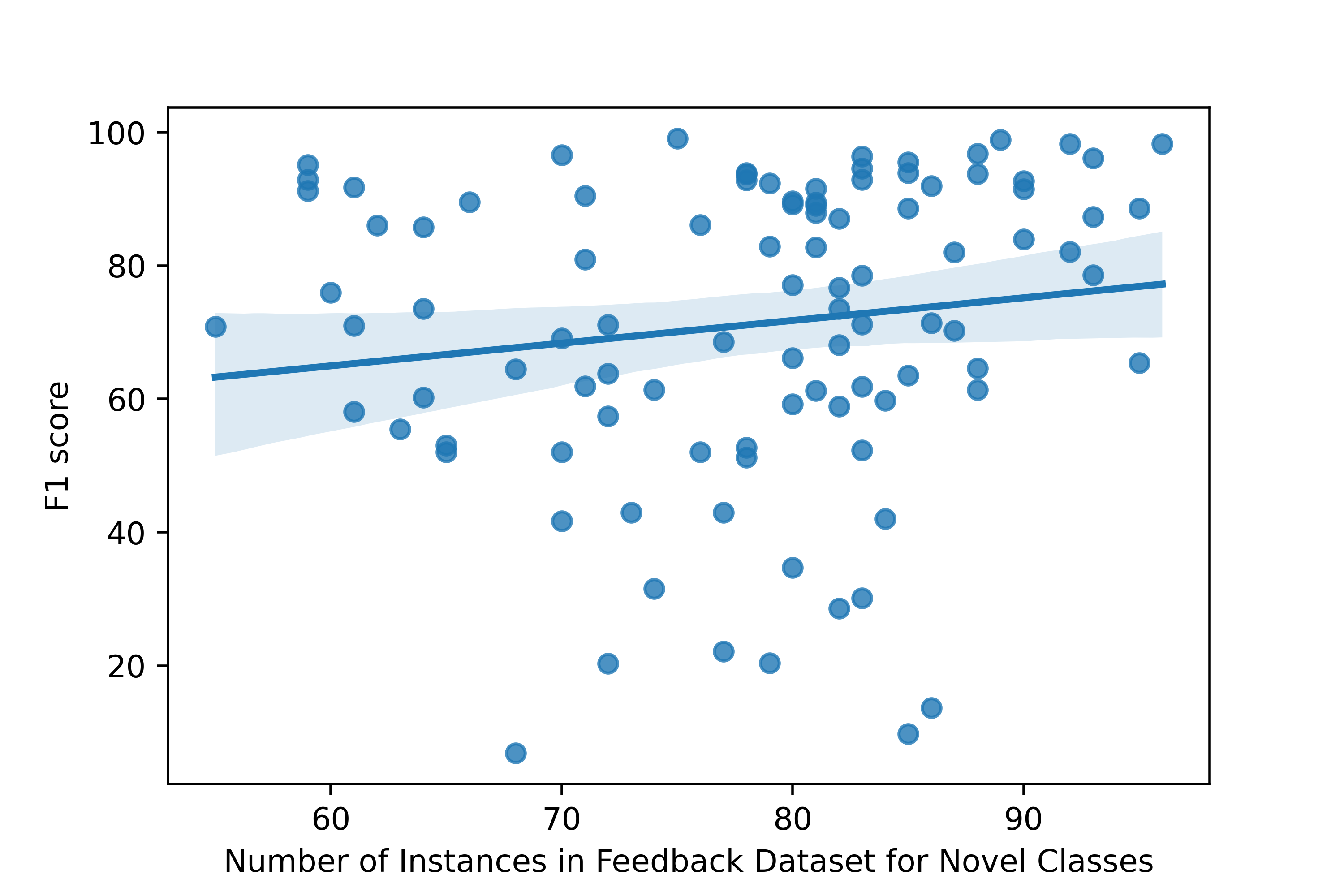
Scatter plot showing F1 performance achieved by each novel class in the accommodation stage vs the number of its instances in the feedback dataset.
The plot is for the MaxProb detection method when 10k novelties are detected for Retrain using and accommodation method.
4.3 Analysis
Distribution of Instances over classes in the Feedback dataset:
We show the distribution of instances over all the classes (novel) in the feedback dataset when the number of reported novelties is 10k in Figure 6.
It can be observed from the histogram that for all the novel classes, novel instances between 55 and 95 are correctly detected. For majority of the classes, 76-85 instances are detected.
This further shows that the detection method is not biased towards or against any set of novel classes in identifying novel instances.
Trend of class level performance in the accommodation stage vs the number of instances in the feedback dataset:
In Figure 7, we show a scatter plot of accommodation F1 performance achieved by each class vs the number of its instances in the feedback dataset.
The plot is for the MaxProb detection method when 10k novelties are detected and retrain with , and accommodation method is used.
From the trend, it can be inferred that with the increase in the number of instances, the performance generally tends to increase.
Comparing Performance of Known and Novel Classes in the Accommodation Stage:
In Figure 8, we compare the performance of the system (in the accommodation stage) on Known and Novel classes.
It clearly shows that the system finds it challenging to adapt itself to the novel classes.
This can be partly attributed to the availability of limited number of training examples of novel classes.
This also provides opportunities for developing better accommodation techniques that can overcome this limitation.
Figure 8:
Comparing Performance on the system on Known and Novel classes in the accommodation stage.
4.4 Other Configuration Settings
In this work, we also study NoveltyTask for different settings (different configuration parameters defined in 4.1).
We observe findings and trends similar to the base setting.
We provide detailed results and discussion in the Appendix.
5 Conclusion and Discussion
To initiate a systematic research in the important yet underexplored area of ‘dealing with novelties’, we introduce NoveltyTask, a multi-stage task to evaluate a system’s performance on pipelined novelty ‘detection’ and ‘accommodation’ tasks.
We provided mathematical formulation of NoveltyTask and instantiated it with the authorship attribution task.
To this end, we also compiled a large dataset (consisting of instances across authors/labels) from Amazon reviews corpus.
We conducted comprehensive experiments and explored several baseline methods for both detection and accommodation tasks.
Looking forward, we believe that our work opens up several avenues for interesting research avenues in this space, such as improving performance of detecting the novel instances and leveraging the feedback in a way that helps the system adapt with just a few examples of the novel labels.
Limitations
Though the formulation of the task allows exploring several different settings (by varying the configuration parameters), in this work, we investigated only the label-balanced setting.
Exploring the label-imbalanced setting is another very interesting research direction, and we leave that for future work.
Another limitation was the limited exploration of novelty detection methods, as a number of methods have been proposed in the recent times. However, we study only a limited set of methods since the focus of this work is on formulating and exploring NoveltyTask.
Lastly, we note that NoveltyTask is a controlled task/framework for evaluating a system’s ability to deal with novelties and not a method to improve its ability.
Acknowledgement
We thank the anonymous reviewers for their insightful feedback. This research was supported by DARPA SAIL-ON program.
References
Aborisade and
Anwar (2018a)
Opeyemi Aborisade and Mohd Anwar. 2018a.
Classification for authorship of tweets by comparing logistic
regression and naive bayes classifiers.
2018 IEEE International Conference on Information Reuse and
Integration (IRI), pages 269–276.
Ai et al. (2022)
Bo Ai, Yuchen Wang, Yugin Tan, and Samson Tan. 2022.
Whodunit?
learning to contrast for authorship attribution.
In Proceedings of the 2nd Conference of the Asia-Pacific
Chapter of the Association for Computational Linguistics and the 12th
International Joint Conference on Natural Language Processing (Volume 1: Long
Papers), pages 1142–1157, Online only. Association for Computational
Linguistics.
Altakrori et al. (2021)
Malik Altakrori, Jackie Chi Kit Cheung, and Benjamin C. M. Fung. 2021.
The
topic confusion task: A novel evaluation scenario for authorship
attribution.
In Findings of the Association for Computational Linguistics:
EMNLP 2021, pages 4242–4256, Punta Cana, Dominican Republic. Association
for Computational Linguistics.
Azizmalayeri and Rohban (2022)
Mohammad Azizmalayeri and Mohammad Hossein Rohban. 2022.
Ood augmentation may be at odds with open-set recognition.
arXiv preprint arXiv:2206.04242.
Bagdon (2021)
Christopher Bagdon. 2021.
Profiling spreaders of hate speech with n-grams and roberta.
In CLEF (Working Notes), pages 1822–1828.
Barlas and Stamatatos (2020)
Georgios Barlas and Efstathios Stamatatos. 2020.
Cross-domain authorship attribution using pre-trained language
models.
In Artificial Intelligence Applications and Innovations, pages
255–266, Cham. Springer International Publishing.
Boenninghoff et al. (2019)
Benedikt Boenninghoff, Steffen Hessler, Dorothea Kolossa, and Robert M Nickel.
2019.
Explainable authorship verification in social media via
attention-based similarity learning.
In 2019 IEEE International Conference on Big Data (Big Data),
pages 36–45. IEEE.
Boult et al. (2020)
Terrance E. Boult, Przemyslaw A. Grabowicz, Derek S. Prijatelj, R. Stern,
Lawrence B. Holder, Joshua Alspector, Mohsen Jafarzadeh, Touqeer Ahmad,
Akshay Raj Dhamija, C.Li, Steve Cruz, A. Shrivastava, Carl Vondrick, and
Walter J. Scheirer. 2020.
A unifying framework for formal theories of novelty: Framework,
examples and discussion.
ArXiv, abs/2012.04226.
Caballero et al. (2021)
Christian Caballero, Hiram Calvo, and Ildar Batyrshin. 2021.
On explainable features for translatorship attribution: Unveiling the
translator’s style with causality.
IEEE Access, 9:93195–93208.
Carpenter and Grossberg (1988)
Gail A. Carpenter and Stephen Grossberg. 1988.
The art of adaptive pattern recognition by a self-organizing neural
network.
Computer, 21(3):77–88.
Chalapathy and Chawla (2019)
Raghavendra Chalapathy and Sanjay Chawla. 2019.
Deep learning for anomaly detection: A survey.
arXiv preprint arXiv:1901.03407.
Custódio and Paraboni (2019)
José Eleandro Custódio and Ivandré Paraboni. 2019.
An ensemble approach to cross-domain authorship attribution.
In Experimental IR Meets Multilinguality, Multimodality, and
Interaction, pages 201–212, Cham. Springer International Publishing.
Devlin et al. (2019)
Jacob Devlin, Ming-Wei Chang, Kenton Lee, and Kristina Toutanova. 2019.
BERT: Pre-training of
deep bidirectional transformers for language understanding.
In Proceedings of the 2019 Conference of the North American
Chapter of the Association for Computational Linguistics: Human Language
Technologies, Volume 1 (Long and Short Papers), pages 4171–4186,
Minneapolis, Minnesota. Association for Computational Linguistics.
Esmaeilpour et al. (2022)
Sepideh Esmaeilpour, Bing Liu, Eric Robertson, and Lei Shu. 2022.
Zero-shot out-of-distribution detection based on the pretrained model
clip.
In Proceedings of the AAAI conference on artificial
intelligence.
Fabien et al. (2020)
Maël Fabien, Esau Villatoro-Tello, Petr Motlicek, and Shantipriya Parida.
2020.
BertAA :
BERT fine-tuning for authorship attribution.
In Proceedings of the 17th International Conference on Natural
Language Processing (ICON), pages 127–137, Indian Institute of Technology
Patna, Patna, India. NLP Association of India (NLPAI).
Fort et al. (2021)
Stanislav Fort, Jie Ren, and Balaji Lakshminarayanan. 2021.
Exploring the limits of out-of-distribution detection.
Advances in Neural Information Processing Systems,
34:7068–7081.
Ghorbani (2019)
Hamid Ghorbani. 2019.
Mahalanobis distance and its application for detecting multivariate
outliers.
Facta Univ Ser Math Inform, 34(3):583–95.
Ghosal et al. (2018)
Tirthankar Ghosal, Vignesh Edithal, Asif Ekbal, Pushpak Bhattacharyya, George
Tsatsaronis, and Srinivasa Satya Sameer Kumar Chivukula. 2018.
Novelty goes deep. a deep
neural solution to document level novelty detection.
In Proceedings of the 27th International Conference on
Computational Linguistics, pages 2802–2813, Santa Fe, New Mexico, USA.
Association for Computational Linguistics.
He and McAuley (2016)
Ruining He and Julian McAuley. 2016.
Ups and downs: Modeling the visual evolution of fashion trends with
one-class collaborative filtering.
In proceedings of the 25th international conference on world
wide web, pages 507–517.
Hendrycks and Gimpel (2017)
Dan Hendrycks and Kevin Gimpel. 2017.
A baseline for detecting misclassified and out-of-distribution
examples in neural networks.
Proceedings of International Conference on Learning
Representations.
Hendrycks et al. (2020)
Dan Hendrycks, Xiaoyuan Liu, Eric Wallace, Adam Dziedzic, Rishabh Krishnan, and
Dawn Song. 2020.
Pretrained
transformers improve out-of-distribution robustness.
In Proceedings of the 58th Annual Meeting of the Association
for Computational Linguistics, pages 2744–2751, Online. Association for
Computational Linguistics.
Jeong et al. (2021)
Minki Jeong, Seokeon Choi, and Changick Kim. 2021.
Few-shot open-set recognition by transformation consistency.
In Proceedings of the IEEE/CVF Conference on Computer Vision
and Pattern Recognition, pages 12566–12575.
Kamath et al. (2020)
Amita Kamath, Robin Jia, and Percy Liang. 2020.
Selective
question answering under domain shift.
In Proceedings of the 58th Annual Meeting of the Association
for Computational Linguistics, pages 5684–5696, Online. Association for
Computational Linguistics.
Krizhevsky (2009)
Alex Krizhevsky. 2009.
Learning multiple layers of features from tiny images.
Technical report.
Lagutina and Lagutina (2021)
Ksenia Lagutina and Nadezhda Lagutina. 2021.
A survey of models for constructing text features to classify texts
in natural language.
In 2021 29th Conference of Open Innovations Association
(FRUCT), pages 222–233. IEEE.
Lagutina et al. (2021)
Ksenia Lagutina, Nadezhda Lagutina, Elena Boychuk, Vladislav Larionov, and Ilya
Paramonov. 2021.
Authorship verification of literary texts with rhythm features.
In 2021 28th Conference of Open Innovations Association
(FRUCT), pages 240–251. IEEE.
Lagutina et al. (2020)
Ksenia Lagutina, Nadezhda Lagutina, Elena Boychuk, and Ilya Paramonov. 2020.
The influence of different stylometric features on the classification
of prose by centuries.
In 2020 27th Conference of Open Innovations Association
(FRUCT), pages 108–115. IEEE.
Li et al. (2022)
Litao Li, Rylen Sampson, Steven HH Ding, and Leo Song. 2022.
Tasr: Adversarial learning of topic-agnostic stylometric
representations for informed crisis response through social media.
Information Processing & Management, 59(2):102857.
Liu et al. (2020)
Bo Liu, Hao Kang, Haoxiang Li, Gang Hua, and Nuno Vasconcelos. 2020.
Few-shot open-set recognition using meta-learning.
In Proceedings of the IEEE/CVF Conference on Computer Vision
and Pattern Recognition, pages 8798–8807.
Liu et al. (2019)
Yinhan Liu, Myle Ott, Naman Goyal, Jingfei Du, Mandar Joshi, Danqi Chen, Omer
Levy, M. Lewis, Luke Zettlemoyer, and Veselin Stoyanov. 2019.
Roberta: A robustly optimized bert pretraining approach.
ArXiv, abs/1907.11692.
Lu et al. (2022)
Jing Lu, Yunlu Xu, Hao Li, Zhanzhan Cheng, and Yi Niu. 2022.
Pmal: Open set recognition via robust prototype mining.
In Proceedings of the AAAI Conference on Artificial
Intelligence, volume 36, pages 1872–1880.
Ma et al. (2021)
Nianzu Ma, Alexander Politowicz, Sahisnu Mazumder, Jiahua Chen, Bing Liu, Eric
Robertson, and Scott Grigsby. 2021.
Semantic
novelty detection in natural language descriptions.
In Proceedings of the 2021 Conference on Empirical Methods in
Natural Language Processing, pages 866–882, Online and Punta Cana,
Dominican Republic. Association for Computational Linguistics.
Manolache et al. (2021)
Andrei Manolache, Florin Brad, Elena Burceanu, Antonio Barbalau, Radu Ionescu,
and Marius Popescu. 2021.
Transferring bert-like transformers’ knowledge for authorship
verification.
arXiv preprint arXiv:2112.05125.
McAuley et al. (2015)
Julian McAuley, Christopher Targett, Qinfeng Shi, and Anton Van Den Hengel.
2015.
Image-based recommendations on styles and substitutes.
In Proceedings of the 38th international ACM SIGIR conference
on research and development in information retrieval, pages 43–52.
Perera et al. (2020)
Pramuditha Perera, Vlad I Morariu, Rajiv Jain, Varun Manjunatha, Curtis
Wigington, Vicente Ordonez, and Vishal M Patel. 2020.
Generative-discriminative feature representations for open-set
recognition.
In Proceedings of the IEEE/CVF Conference on Computer Vision
and Pattern Recognition, pages 11814–11823.
Qin et al. (2020)
Qi Qin, Wenpeng Hu, and Bing Liu. 2020.
Text classification with novelty detection.
arXiv preprint arXiv:2009.11119.
Rambhatla et al. (2021)
Sai Saketh Rambhatla, Ramalingam Chellappa, and Abhinav Shrivastava. 2021.
The pursuit of knowledge: Discovering and localizing novel categories
using dual memory.
2021 IEEE/CVF International Conference on Computer Vision
(ICCV), pages 9133–9143.
Sari et al. (2018)
Yunita Sari, Mark Stevenson, and Andreas Vlachos. 2018.
Topic or style? exploring
the most useful features for authorship attribution.
In Proceedings of the 27th International Conference on
Computational Linguistics, pages 343–353, Santa Fe, New Mexico, USA.
Association for Computational Linguistics.
Soler-Company and Wanner (2017)
Juan Soler-Company and Leo Wanner. 2017.
On the relevance of
syntactic and discourse features for author profiling and identification.
In Proceedings of the 15th Conference of the European Chapter
of the Association for Computational Linguistics: Volume 2, Short Papers,
pages 681–687, Valencia, Spain. Association for Computational Linguistics.
Sun et al. (2021a)
Xin Sun, Henghui Ding, Chi Zhang, Guosheng Lin, and Keck-Voon Ling.
2021a.
M2iosr: Maximal mutual information open set recognition.
arXiv preprint arXiv:2108.02373.
Sun et al. (2020)
Xin Sun, Zhenning Yang, Chi Zhang, Keck-Voon Ling, and Guohao Peng. 2020.
Conditional gaussian distribution learning for open set recognition.
In Proceedings of the IEEE/CVF Conference on Computer Vision
and Pattern Recognition, pages 13480–13489.
Sun et al. (2021b)
Yiyou Sun, Chuan Guo, and Yixuan Li. 2021b.
React: Out-of-distribution detection with rectified activations.
Advances in Neural Information Processing Systems,
34:144–157.
Tyo et al. (2021)
Jacob Tyo, Bhuwan Dhingra, and Zachary C Lipton. 2021.
Siamese bert for authorship verification.
In CLEF (Working Notes), pages 2169–2177.
Varshney and Baral (2022)
Neeraj Varshney and Chitta Baral. 2022.
Model
cascading: Towards jointly improving efficiency and accuracy of NLP
systems.
In Proceedings of the 2022 Conference on Empirical Methods in
Natural Language Processing, pages 11007–11021, Abu Dhabi, United Arab
Emirates. Association for Computational Linguistics.
Varshney and Baral (2023)
Neeraj Varshney and Chitta Baral. 2023.
Post-abstention: Towards reliably re-attempting the abstained
instances in qa.
arXiv preprint arXiv:2305.01812.
Varshney et al. (2022a)
Neeraj Varshney, Man Luo, and Chitta Baral. 2022a.
Can open-domain qa reader utilize external knowledge efficiently like
humans?
arXiv preprint arXiv:2211.12707.
Varshney et al. (2022c)
Neeraj Varshney, Swaroop Mishra, and Chitta Baral. 2022c.
Towards
improving selective prediction ability of NLP systems.
In Proceedings of the 7th Workshop on Representation Learning
for NLP, pages 221–226, Dublin, Ireland. Association for Computational
Linguistics.
Venkataram (2018)
Vinodini Molukuvan Venkataram. 2018.
Open set text classification using neural networks.
University of Colorado Colorado Springs.
Wang and Iwaihara (2021)
Xiangyu Wang and Mizuho Iwaihara. 2021.
Integrating roberta fine-tuning and user writing styles for
authorship attribution of short texts.
In Web and Big Data, pages 413–421, Cham. Springer
International Publishing.
Wei et al. (2021)
Hongxin Wei, Lue Tao, Renchunzi Xie, and Bo An. 2021.
Open-set label noise can improve robustness against inherent label
noise.
Advances in Neural Information Processing Systems,
34:7978–7992.
Whitehead et al. (2022)
Spencer Whitehead, Suzanne Petryk, Vedaad Shakib, Joseph Gonzalez, Trevor
Darrell, Anna Rohrbach, and Marcus Rohrbach. 2022.
Reliable visual question answering: Abstain rather than answer
incorrectly.
In Proceedings of the European Conference on Computer Vision
(ECCV).
Xin et al. (2021)
Ji Xin, Raphael Tang, Yaoliang Yu, and Jimmy Lin. 2021.
The art of
abstention: Selective prediction and error regularization for natural
language processing.
In Proceedings of the 59th Annual Meeting of the Association
for Computational Linguistics and the 11th International Joint Conference on
Natural Language Processing (Volume 1: Long Papers), pages 1040–1051,
Online. Association for Computational Linguistics.
Xu et al. (2019)
Hu Xu, Bing Liu, Lei Shu, and P Yu. 2019.
Open-world learning and application to product classification.
In The World Wide Web Conference, pages 3413–3419.
Yang et al. (2022)
Shiqi Yang, Yaxing Wang, Kai Wang, Shangling Jui, and Joost van de Weijer.
2022.
One ring to bring them all: Towards open-set recognition under domain
shift.
arXiv preprint arXiv:2206.03600.
Yilmaz and Toraman (2022)
Eyup Yilmaz and Cagri Toraman. 2022.
D2u: Distance-to-uniform learning for out-of-scope detection.
In Proceedings of the 2022 Conference of the North American
Chapter of the Association for Computational Linguistics: Human Language
Technologies, pages 2093–2108.
Zhou et al. (2021a)
Da-Wei Zhou, Han-Jia Ye, and De-Chuan Zhan. 2021a.
Learning
placeholders for open-set recognition.
In 2021 IEEE/CVF Conference on Computer Vision and Pattern
Recognition (CVPR), pages 4399–4408.
Zhou et al. (2021b)
Da-Wei Zhou, Han-Jia Ye, and De-Chuan Zhan. 2021b.
Learning placeholders for open-set recognition.
In Proceedings of the IEEE/CVF Conference on Computer Vision
and Pattern Recognition, pages 4401–4410.
Zhou et al. (2021c)
Wenxuan Zhou, Fangyu Liu, and Muhao Chen. 2021c.
Contrastive
out-of-distribution detection for pretrained transformers.
In Proceedings of the 2021 Conference on Empirical Methods in
Natural Language Processing, pages 1100–1111, Online and Punta Cana,
Dominican Republic. Association for Computational Linguistics.
Fort et al. 2021 demonstrated that pre-training of transformer-based models using large datasets is fairly robust in detecting near-OOD instances using few examples.
Esmaeilpour et al. 2022 proposed to detect OOD instances using pairwise similarity score. They generate synthetic unseen examples and use their closed-set classifier to compute pairwise similarity.
Wei et al. 2021 use open-set samples with dynamic, noisy labels and assign random labels to open-set examples, and use them for developing a system for OOD detection.
Sun et al. 2021b analyze activation functions of the penultimate layer of pretrained models and rectify the activations to an upper limit for OOD detection.
A.1.2 Language
Zhou et al. 2021b propose to add an additional classifier in addition to a closed domain classifier for getting a class-specific threshold of known and unknown classes. They generate data placeholders to mimic open set categories.
Venkataram 2018 use an ensemble-based approach and replace the softmax layer with an OpenMAX layer.
The hypothesis is that the closest (most similar) class to any known class is an unknown one. This allows the classifier to be trained, enforcing the most probable class to be the ground truth class and the runner-up class to be the background class for all source data.
Zhou et al. 2021c employ a contrastive learning framework for unsupervised OOD detection, which is composed of a contrastive loss and an OOD scoring function. The contrastive loss increases the discrepancy of the representations of instances from different classes in the task, while the OOD scoring function maps the representations of instances to OOD detection scores.
Xu et al. 2019 propose Learning to Accept Classes (L2AC) method based on meta-learning and does not require re-training the model when new classes are added.
L2AC works by maintaining a set of seen classes and comparing new data points to the nearest example from each seen class.
BERT (and its different variants like BertAA, RoBERTa) based, Siamese-based, and ensemble-based approaches have been used for authorship attribution.
Tyo et al. 2021 propose an approach that uses a pretrained BERT model in a siamese configuration for audio-visual classification.
They experiment with using triplet loss, contrastive loss, and a modified version of contrastive loss and compare the results.
Bagdon 2021 combine the results of a n-gram-based logistic regression classifier with a transformer model based on RoBERTa Liu et al. 2019 via a SVM meta-classifier.
Altakrori et al. 2021 explore a new evaluation setting topic confusion task.
The topic distribution is controlled by making it dependent on the author, switching the topic-author pairs between training and testing. This setup allows for measuring the degree to which certain features are influenced by the topic, as opposed to the author’s identity.
Other works include Barlas and Stamatatos 2020; Fabien et al. 2020; Wang and Iwaihara 2021. N-grams, word embeddings, and other stylometric features have been used as input feature vectors for the task Caballero et al. 2021; Boenninghoff et al. 2019; Li et al. 2022; Lagutina et al. 2021; Lagutina et al. 2020; Lagutina and Lagutina 2021.
Appendix B Novelty Detection Algorithms
Learning placeholders:
The Placeholders algorithm consists of two main components: "Learning Classifier Placeholders" and "Learning Data Placeholders". "Learning Classifier Placeholders" involves adding a set of weights called classifier placeholders to the linear classifier layer at the end of the network. This modified classifier function denoted as , where w represents the weights of the additional k+1 class, is trained using a modified loss function that encourages the classifier to predict the k+1 class as the second most likely class for every sample. This loss function helps the classifier learn an embedding function such that the k+1 class is always the closest class to each class cluster boundary. In addition to the k+1 class, the Placeholders algorithm includes a tunable number (C) of additional classifiers to make decisions’ boundaries smoother. The final classifier function is, therefore, , meaning that the closest open-set region in the embedding space is taken into consideration.
"Learning Data Placeholders" involves tightening the decision boundaries around the known-class clusters in the embedding space through a process called manifold mixup. This involves creating "unknown" class data from known class data and using an additional loss function to penalize classifying this new data as any of the known classes. Manifold mixup works by interpolating the embeddings of two samples from closed-set classes to create an embedding for a new sample, which is considered to belong to an unknown class. After training the model using both classifier and data placeholders, the Placeholders algorithm includes a final calibration step in which an additional bias is added to the open-set logits. This bias is tuned using a validation set of closed-set samples such that 95% of all closed-set samples are classified as known. The combination of these two components and final calibration allows the Placeholders algorithm to train a classifier to identify novel samples even when only trained on closed-set data.
Few Shot Open set Recognition using Meta-Learning
: In the paper "Few-Shot Open-Set Recognition using Meta-Learning", the authors propose a method for few-shot open-set recognition using meta-learning. The main idea is to train a meta-learner that can recognize new classes given a few examples of each class.
The meta-learner consists of a feature extractor network and a linear classifier. The feature extractor network is responsible for learning an embedding function that maps samples from different classes into a common embedding space. The goal is to learn an embedding function that clusters samples from the same class together while separating samples from different classes by a large margin.
To train the meta-learner, the authors use a meta-learning loss function that encourages the embedding function to learn a "smooth" embedding space. This loss function consists of two terms: a classification loss and a separation loss.
During training, the meta-learner is presented with a small number of examples from each new class and is required to classify these examples correctly. The meta-learner is trained to optimize the meta-learning loss function, which encourages the embedding function to learn a smooth embedding space where samples from different classes are well separated.
After training, the meta-learner can be used to classify new samples by first projecting them into the embedding space using the feature extractor network, and then using the linear classifier to assign them to the appropriate class. The final classifier is able to generalize to new classes not seen during training, as it has learned to recognize the underlying structure of the embedding space.
Appendix C Results
Hyperparameters of the model:
Hidden layer dropout probability of 0.15,
input Sequence length of 512 tokens,
batch size of 32, and standard learning rate ranging in .
C.1 Novelty Accomodation Stage
Table 1, 2, and 3 show the results of all six novelty detection methods across all three accommodation settings on the first dataset whose results are described in details in the main paper.
Similar results are obtained for datasets 2 and 3 as well.
Novelty Accommodation results for dataset 2 are present in table 4, 5, and 6 and in table 7, 8, and 9 for dataset 3.
# of
Novelties
Known
Class
precision
Known
class
recall
Known
Class
F1
Novel
Class
Precision
Novel
Class
Recall
Novel
Class
F1
Overall
Precision
Overall
Recall
Overall
F1
1000
51.62
90.10
65.64
15.62
2.23
3.90
33.62
46.17
38.91
2000
54.17
90.62
67.81
30.21
8.51
13.28
42.19
49.56
45.58
3000
55.25
89.92
68.44
50.29
12.69
20.27
52.77
51.31
52.03
4000
58.64
89.61
70.89
67.22
23.97
35.34
62.93
56.79
59.70
5000
60.77
90.16
72.60
74.02
30.99
43.69
67.40
60.58
63.81
6000
62.60
89.59
73.70
76.85
36.23
49.24
69.73
62.91
66.14
7000
64.90
89.62
75.28
80.26
42.21
55.32
72.58
65.92
69.09
8000
67.03
89.61
76.69
82.63
48.16
60.85
74.83
68.89
71.74
9000
67.90
89.35
77.16
82.83
50.46
62.71
75.37
69.91
72.54
10000
69.91
89.67
78.57
83.81
54.10
65.75
76.86
71.89
74.29
Compute Mean
1000
55.57
89.67
68.62
6.41
7.71
7.00
30.99
48.69
37.87
2000
55.86
90.10
68.96
9.09
10.98
9.95
32.48
50.54
39.55
3000
57.29
89.92
69.99
13.54
15.52
14.46
35.42
52.72
42.37
4000
58.63
89.40
70.82
15.88
18.07
16.90
37.26
53.74
44.01
5000
59.39
89.72
71.47
19.00
20.82
19.87
39.19
55.27
45.86
6000
61.03
89.34
72.52
23.67
25.77
24.68
42.35
57.56
48.80
7000
61.67
89.63
73.07
27.36
28.05
27.70
44.51
58.84
50.68
8000
63.27
89.30
74.06
31.58
32.01
31.79
47.42
60.66
53.23
9000
64.12
89.15
74.59
35.75
34.22
34.97
49.93
61.69
55.19
10000
65.70
89.18
75.66
40.30
38.12
39.18
53.00
63.65
57.84
Compute Euclid Distance
1000
54.84
90.10
68.18
30.39
11.45
16.63
42.61
50.78
46.34
2000
59.14
90.22
71.45
56.80
21.40
31.09
57.97
55.81
56.87
3000
62.09
90.02
73.49
73.87
31.43
44.10
67.98
60.72
64.15
4000
64.82
89.66
75.24
78.40
39.37
52.42
71.61
64.51
67.87
5000
67.45
89.29
76.85
80.12
47.33
59.51
73.78
68.31
70.94
6000
69.63
89.93
78.49
83.73
54.05
65.69
76.68
71.99
74.26
7000
71.18
89.45
79.28
83.37
57.08
67.76
77.27
73.26
75.21
8000
71.48
89.20
79.36
83.93
58.09
68.66
77.71
73.64
75.62
9000
72.10
89.09
79.70
84.41
60.30
70.35
78.26
74.69
76.43
10000
73.45
88.92
80.45
85.03
62.08
71.76
79.24
75.50
77.32
Compute Mahalanobis Distance
1000
54.72
89.65
67.96
29.72
9.65
14.57
42.22
49.65
45.63
2000
59.75
90.12
71.86
55.68
22.54
32.09
57.72
56.33
57.02
3000
61.80
89.69
73.18
66.02
31.36
42.52
63.91
60.53
62.17
4000
64.73
90.20
75.37
75.62
39.72
52.08
70.17
64.96
67.46
5000
67.11
89.53
76.72
80.63
46.47
58.96
73.87
68.00
70.81
6000
69.20
89.61
78.09
82.91
51.50
63.53
76.06
70.56
73.21
7000
70.90
89.39
79.08
83.39
55.98
66.99
77.14
72.68
74.84
8000
71.13
89.20
79.15
84.92
58.64
69.37
78.03
73.92
75.92
9000
73.21
89.59
80.58
85.68
61.90
71.87
79.44
75.75
77.55
10000
73.92
89.11
80.81
86.08
64.00
73.42
80.00
76.55
78.24
Compute Max Probability
1000
53.87
89.72
67.32
17.00
7.15
10.07
35.44
48.43
40.93
2000
56.30
90.26
69.35
33.36
16.72
22.28
44.83
53.49
48.78
3000
59.59
89.59
71.57
56.36
24.13
33.79
57.97
56.86
57.41
4000
62.23
89.46
73.40
69.30
34.70
46.24
65.77
62.08
63.87
5000
66.08
89.81
76.14
76.18
44.24
55.97
71.13
67.03
69.02
6000
68.11
89.66
77.41
84.26
50.07
62.81
76.18
69.86
72.88
7000
69.64
89.52
78.34
83.82
54.43
66.00
76.73
71.97
74.27
8000
72.31
89.36
79.94
85.28
59.61
70.17
78.80
74.48
76.58
9000
73.03
89.30
80.35
85.77
62.45
72.28
79.40
75.87
77.59
10000
74.69
88.94
81.19
85.24
65.03
73.78
79.96
76.98
78.44
Placeholders Algorithm
1000
54.45
90.31
67.94
29.47
10.84
15.85
41.96
50.57
45.86
2000
57.17
90.10
69.95
44.44
18.82
26.44
50.80
54.46
52.57
3000
61.10
89.96
72.77
55.81
29.59
38.67
58.45
59.77
59.10
4000
62.74
89.85
73.89
73.03
36.60
48.76
67.88
63.23
65.47
5000
65.90
89.69
75.98
79.94
43.86
56.64
72.92
66.77
69.71
6000
67.59
89.34
76.96
83.69
49.98
62.58
75.64
69.66
72.53
7000
70.52
89.73
78.97
84.42
56.92
67.99
77.47
73.33
75.34
8000
71.90
89.64
79.80
85.32
59.24
69.93
78.61
74.44
76.47
9000
72.34
89.04
79.83
83.72
58.95
69.18
78.03
73.99
75.96
10000
73.41
89.71
80.75
85.84
61.92
71.94
79.63
75.81
77.67
Few shot Open set Recognition
Table 1:
Novelty Accommodation Stage: Dataset 1: Retrain using and
# of
Novelties
Known
Class
precision
Known
class
recall
Known
Class
F1
Novel
Class
Precision
Novel
Class
Recall
Novel
Class
F1
Overall
Precision
Overall
Recall
Overall
F1
1000
74.55
26.02
38.58
3.43
4.92
4.04
38.99
15.47
22.15
2000
61.86
18.28
28.22
11.74
15.12
13.22
36.80
16.70
22.97
3000
75.14
23.99
36.37
27.67
25.67
26.63
51.41
24.83
33.49
4000
73.70
20.93
32.60
34.57
38.53
36.44
54.14
29.73
38.38
5000
77.08
19.84
31.56
40.72
48.88
44.43
58.90
34.36
43.40
6000
72.90
19.24
30.44
43.49
57.53
49.53
58.19
38.38
46.25
7000
61.77
8.98
15.68
44.02
61.30
51.24
52.90
35.14
42.23
8000
58.13
8.69
15.12
47.92
66.64
55.75
53.03
37.66
44.04
9000
53.48
6.53
11.64
48.35
69.98
57.19
50.91
38.25
43.68
10000
38.57
6.35
10.90
48.24
71.15
57.50
43.41
38.75
40.95
Compute Mean
1000
39.95
6.68
11.45
1.03
9.21
1.85
20.49
7.95
11.46
2000
16.75
1.06
1.99
2.01
13.72
3.51
9.38
7.39
8.27
3000
27.00
3.90
6.82
3.91
18.67
6.47
15.45
11.29
13.05
4000
23.00
1.59
2.97
4.62
21.82
7.63
13.81
11.71
12.67
5000
19.92
1.56
2.89
5.25
24.94
8.67
12.59
13.25
12.91
6000
11.00
0.87
1.61
8.57
30.25
13.36
9.79
15.56
12.02
7000
20.67
3.02
5.27
11.31
33.58
16.92
15.99
18.30
17.07
8000
11.00
0.75
1.40
12.96
37.76
19.30
11.98
19.26
14.77
9000
11.00
0.11
0.22
15.43
41.53
22.50
13.22
20.82
16.17
10000
12.00
0.32
0.62
18.28
45.52
26.08
15.14
22.92
18.23
Compute Euclid Distance
1000
79.11
40.70
53.75
17.10
16.37
16.73
48.10
28.54
35.82
2000
85.75
35.22
49.93
35.85
31.74
33.67
60.80
33.48
43.18
3000
76.62
17.90
29.02
46.81
44.39
45.57
61.72
31.14
41.39
4000
72.88
13.35
22.57
47.42
56.88
51.72
60.15
35.11
44.34
5000
59.96
11.48
19.27
49.27
67.04
56.80
54.62
39.26
45.68
6000
43.27
6.98
12.02
49.74
70.48
58.32
46.50
38.73
42.26
7000
33.50
3.19
5.83
48.67
73.52
58.57
41.09
38.35
39.67
8000
35.45
4.49
7.97
49.63
75.66
59.94
42.54
40.08
41.27
9000
26.33
2.93
5.27
50.30
78.02
61.17
38.32
40.47
39.37
10000
17.00
3.14
5.30
51.87
79.31
62.72
34.43
41.23
37.52
Compute Mahalanobis Distance
1000
77.64
31.72
45.04
11.59
15.90
13.41
44.61
23.81
31.05
2000
79.25
22.94
35.58
27.57
32.88
29.99
53.41
27.91
36.66
3000
88.60
23.51
37.16
35.89
42.37
38.86
62.25
32.94
43.08
4000
78.20
10.35
18.28
42.53
56.15
48.40
60.37
33.25
42.88
5000
50.86
7.91
13.69
45.89
60.54
52.21
48.38
34.23
40.09
6000
50.45
6.47
11.47
47.37
70.73
56.74
48.91
38.60
43.15
7000
27.26
2.83
5.13
47.90
74.23
58.23
37.58
38.53
38.05
8000
21.00
2.65
4.71
49.53
77.02
60.29
35.27
39.83
37.41
9000
22.00
3.56
6.13
50.31
78.15
61.21
36.15
40.85
38.36
10000
17.97
1.25
2.34
51.21
80.49
62.60
34.59
40.87
37.47
Compute Max Probability
1000
64.52
20.06
30.60
3.20
6.38
4.26
33.86
13.22
19.02
2000
84.61
25.01
38.61
18.63
22.15
20.24
51.62
23.58
32.37
3000
57.24
11.32
18.90
24.95
35.16
29.19
41.10
23.24
29.69
4000
63.88
11.03
18.81
36.70
47.23
41.30
50.29
29.13
36.89
5000
56.02
6.07
10.95
42.32
58.27
49.03
49.17
32.17
38.89
6000
43.84
5.29
9.44
45.00
65.42
53.32
44.42
35.35
39.37
7000
37.02
5.00
8.81
47.77
71.41
57.25
42.39
38.21
40.19
8000
28.85
4.55
7.86
48.98
75.65
59.46
38.91
40.10
39.50
9000
16.00
1.86
3.33
49.15
78.29
60.39
32.58
40.07
35.94
10000
19.90
2.05
3.72
51.34
79.65
62.44
35.62
40.85
38.06
Placeholders Algorithm
1000
75.81
26.33
39.09
5.38
10.21
7.05
40.60
18.27
25.20
2000
83.63
24.58
37.99
18.81
27.74
22.42
51.22
26.16
34.63
3000
84.29
19.97
32.29
28.87
40.48
33.70
56.58
30.23
39.41
4000
59.16
9.35
16.15
35.60
50.84
41.88
47.38
30.09
36.81
5000
60.67
6.64
11.97
42.08
59.11
49.16
51.38
32.87
40.09
6000
50.79
5.49
9.91
48.35
69.81
57.13
49.57
37.65
42.80
7000
29.00
3.19
5.75
47.59
74.18
57.98
38.30
38.68
38.49
8000
26.99
3.25
5.80
48.55
73.98
58.63
37.77
38.62
38.19
9000
25.70
2.20
4.05
50.46
77.10
61.00
38.08
39.65
38.85
10000
19.94
1.77
3.25
49.57
78.38
60.73
34.76
40.07
37.23
Few shot Open set Recognition
Table 2:
Novelty Accommodation Stage: Dataset 1: Further Fine-tune using .
# of
Novelties
Known
Class
precision
Known
class
recall
Known
Class
F1
Novel
Class
Precision
Novel
Class
Recall
Novel
Class
F1
Overall
Precision
Overall
Recall
Overall
F1
1000
59.69
87.26
70.89
15.37
4.64
7.13
37.53
45.95
41.32
2000
62.66
87.70
73.09
32.20
14.14
19.65
47.43
50.92
49.11
3000
65.50
86.96
74.72
48.58
22.47
30.73
57.04
54.72
55.86
4000
68.97
87.08
76.97
62.66
34.79
44.74
65.81
60.94
63.28
5000
73.44
86.87
79.59
65.70
44.87
53.32
69.57
65.87
67.67
6000
75.33
85.70
80.18
67.43
51.22
58.22
71.38
68.46
69.89
7000
78.45
85.66
81.90
70.25
57.98
63.53
74.35
71.82
73.06
8000
80.33
85.03
82.61
72.67
62.59
67.25
76.50
73.81
75.13
9000
81.31
84.65
82.95
73.82
66.87
70.17
77.56
75.76
76.65
10000
82.88
84.44
83.65
74.13
68.83
71.38
78.50
76.64
77.56
Compute Mean
1000
57.36
88.99
69.76
3.95
8.73
5.44
30.66
48.86
37.68
2000
60.92
88.75
72.25
5.96
12.81
8.14
33.44
50.78
40.32
3000
63.45
88.03
73.75
9.74
17.96
12.63
36.60
52.99
43.30
4000
65.72
87.84
75.19
11.33
20.86
14.68
38.52
54.35
45.09
5000
65.68
87.91
75.19
13.52
23.76
17.23
39.60
55.83
46.33
6000
68.42
87.28
76.71
18.28
28.87
22.39
43.35
58.08
49.65
7000
69.71
86.83
77.33
21.18
31.86
25.44
45.44
59.34
51.47
8000
71.32
87.33
78.52
25.46
35.86
29.78
48.39
61.60
54.20
9000
73.99
86.78
79.88
28.26
39.38
32.91
51.12
63.08
56.47
10000
75.89
86.23
80.73
32.54
43.27
37.15
54.21
64.75
59.01
Compute Euclid Distance
1000
63.23
87.81
73.52
30.48
15.33
20.40
46.86
51.57
49.10
2000
68.99
87.47
77.14
52.53
28.39
36.86
60.76
57.93
59.31
3000
72.93
86.67
79.21
64.15
42.46
51.10
68.54
64.57
66.50
4000
75.98
86.22
80.78
70.70
53.82
61.12
73.34
70.02
71.64
5000
79.22
85.36
82.18
73.09
62.86
67.59
76.15
74.11
75.12
6000
81.70
85.02
83.33
74.91
68.35
71.48
78.31
76.69
77.49
7000
82.01
85.48
83.71
76.69
70.31
73.36
79.35
77.89
78.61
8000
82.80
85.56
84.16
77.90
72.09
74.88
80.35
78.83
79.58
9000
83.54
84.62
84.08
77.92
73.29
75.53
80.73
78.95
79.83
10000
84.50
84.31
84.40
78.39
75.05
76.68
81.45
79.68
80.56
Compute Mahalanobis Distance
1000
61.52
88.11
72.45
32.72
16.57
22.00
47.12
52.34
49.59
2000
68.34
87.25
76.65
49.43
30.10
37.42
58.89
58.67
58.78
3000
73.16
86.78
79.39
61.57
41.30
49.44
67.36
64.04
65.66
4000
76.49
86.25
81.08
67.36
51.58
58.42
71.93
68.92
70.39
5000
78.93
85.77
82.21
72.94
61.55
66.76
75.94
73.66
74.78
6000
80.99
85.69
83.27
74.78
66.77
70.55
77.88
76.23
77.05
7000
81.71
84.69
83.17
75.56
68.76
72.00
78.63
76.72
77.66
8000
83.11
85.45
84.26
77.29
72.60
74.87
80.20
79.03
79.61
9000
83.76
84.45
84.10
77.86
73.79
75.77
80.81
79.12
79.96
10000
84.55
84.18
84.36
78.58
75.10
76.80
81.57
79.64
80.59
Compute Max Probability
1000
58.20
88.66
70.27
23.09
12.71
16.40
40.65
50.69
45.12
2000
65.05
88.25
74.89
37.00
26.00
30.54
51.02
57.12
53.90
3000
68.66
87.88
77.09
57.39
35.26
43.68
63.03
61.57
62.29
4000
73.22
87.58
79.76
64.21
47.60
54.67
68.71
67.59
68.15
5000
77.43
86.70
81.80
70.83
57.74
63.62
74.13
72.22
73.16
6000
79.69
86.50
82.96
74.79
63.95
68.95
77.24
75.23
76.22
7000
81.81
85.93
83.82
76.06
69.15
72.44
78.93
77.54
78.23
8000
82.86
85.38
84.10
76.89
71.83
74.27
79.88
78.60
79.23
9000
84.09
85.00
84.54
77.74
74.36
76.01
80.91
79.68
80.29
10000
84.60
84.47
84.53
78.24
75.36
76.77
81.42
79.91
80.66
Placeholders Algorithm
1000
58.94
88.66
70.81
28.65
17.12
21.43
43.80
52.89
47.92
2000
64.40
88.71
74.63
49.10
27.78
35.48
56.75
58.25
57.49
3000
68.68
88.11
77.19
59.69
38.73
46.98
64.19
63.42
63.80
4000
72.46
87.32
79.20
68.83
46.58
55.56
70.64
66.95
68.75
5000
75.73
87.02
80.98
75.08
58.55
65.79
75.41
72.79
74.08
6000
79.48
85.99
82.61
75.94
65.82
70.52
77.71
75.91
76.80
7000
81.18
85.87
83.46
77.52
69.19
73.12
79.35
77.53
78.43
8000
83.05
85.40
84.21
78.70
73.36
75.94
80.87
79.38
80.12
9000
82.48
85.17
83.80
78.39
72.41
75.28
80.44
78.79
79.61
10000
83.14
85.43
84.27
78.92
73.88
76.32
81.03
79.65
80.33
Few shot Open set Recognition
Table 3:
Novelty Accommodation Stage: Dataset 1: Further Fine-tune using Sampled and .
# of
Novelties
Known
Class
precision
Known
class
recall
Known
Class
F1
Novel
Class
Precision
Novel
Class
Recall
Novel
Class
F1
Overall
Precision
Overall
Recall
Overall
F1
4000
57.47
89.90
70.12
57.28
20.96
30.69
57.38
55.43
56.39
8000
66.31
88.96
75.98
83.59
45.46
58.89
74.95
67.21
70.87
12000
71.26
88.93
79.12
85.16
57.43
68.60
78.21
73.18
75.61
16000
75.42
89.55
81.88
86.76
67.05
75.64
81.09
78.30
79.67
20000
77.47
89.41
83.01
88.40
71.43
79.01
82.94
80.42
81.66
Compute Mean
4000
56.84
89.63
69.56
9.09
12.39
10.49
32.96
51.01
40.05
8000
60.52
89.47
72.20
15.40
21.08
17.80
37.96
55.27
45.01
12000
62.75
89.67
73.83
23.36
28.78
25.79
43.06
59.22
49.86
16000
66.27
89.51
76.16
31.26
36.25
33.57
48.77
62.88
54.93
20000
68.62
89.19
77.56
40.37
43.76
42.00
54.49
66.47
59.89
Compute Euclid Distance
4000
65.56
89.81
75.79
73.37
39.72
51.54
69.47
64.77
67.04
8000
73.69
89.30
80.75
85.84
63.55
73.03
79.77
76.43
78.06
12000
77.47
89.19
82.92
88.01
71.65
78.99
82.74
80.42
81.56
16000
79.19
88.81
83.72
88.18
74.73
80.90
83.68
81.77
82.71
20000
80.33
88.63
84.28
89.57
77.62
83.17
84.95
83.12
84.03
Compute Mahalanobis Distance
4000
65.24
89.96
75.63
75.98
38.95
51.50
70.61
64.46
67.39
8000
73.35
89.48
80.62
85.56
61.38
71.48
79.45
75.43
77.39
12000
76.74
89.29
82.54
87.99
70.02
77.98
82.37
79.66
80.99
16000
80.08
89.05
84.33
89.10
76.62
82.39
84.59
82.83
83.70
20000
80.83
89.01
84.72
90.47
78.57
84.10
85.65
83.79
84.71
Compute Max Probability
4000
61.55
90.02
73.11
58.92
28.77
38.66
60.24
59.40
59.82
8000
70.28
89.56
78.76
82.11
53.64
64.89
76.19
71.60
73.82
12000
76.39
88.87
82.16
87.62
68.74
77.04
82.00
78.80
80.37
16000
80.09
89.08
84.35
88.95
76.14
82.05
84.52
82.61
83.55
20000
81.25
88.80
84.86
89.25
78.42
83.49
85.25
83.61
84.42
Placeholders Algorithm
4000
61.32
89.86
72.90
57.04
30.12
39.42
59.18
59.99
59.58
8000
69.68
89.87
78.50
85.11
52.89
65.24
77.39
71.38
74.26
12000
74.92
89.04
81.37
87.46
65.95
75.20
81.19
77.50
79.30
16000
78.69
88.63
83.36
88.87
74.19
80.87
83.78
81.41
82.58
20000
80.82
88.82
84.63
90.20
78.17
83.76
85.51
83.49
84.49
Few shot Open set Recognition
Table 4:
Novelty Accommodation Stage: Dataset 2: Retrain using and
# of
Novelties
Known
Class
precision
Known
class
recall
Known
Class
F1
Novel
Class
Precision
Novel
Class
Recall
Novel
Class
F1
Overall
Precision
Overall
Recall
Overall
F1
4000
83.55
28.67
42.69
33.25
32.69
32.97
58.40
30.68
40.23
8000
48.80
7.04
12.30
45.59
61.05
52.20
47.20
34.05
39.56
12000
36.71
4.56
8.11
49.62
75.64
59.93
43.17
40.10
41.58
16000
18.00
2.26
4.02
53.16
80.24
63.95
35.58
41.25
38.21
20000
10.00
3.27
4.93
55.63
84.25
67.01
32.81
43.76
37.50
Compute Mean
4000
12.89
0.76
1.44
1.90
14.41
3.36
7.39
7.58
7.48
8000
6.00
1.75
2.71
4.59
22.88
7.65
5.29
12.32
7.40
12000
13.98
2.31
3.96
8.50
31.69
13.40
11.24
17.00
13.53
16000
7.76
0.22
0.43
13.20
39.82
19.83
10.48
20.02
13.76
20000
10.00
0.13
0.26
19.13
48.70
27.47
14.57
24.42
18.25
Compute Euclid Distance
4000
79.08
15.55
25.99
45.61
54.41
49.62
62.34
34.98
44.81
8000
30.00
3.81
6.76
51.96
79.00
62.69
40.98
41.41
41.19
12000
15.00
1.50
2.73
54.29
84.03
65.96
34.65
42.76
38.28
16000
10.00
0.75
1.40
55.82
86.85
67.96
32.91
43.80
37.58
20000
4.00
0.42
0.76
55.57
87.67
68.02
29.78
44.04
35.53
Compute Mahalanobis Distance
4000
64.78
14.62
23.86
43.47
52.66
47.63
54.12
33.64
41.49
8000
27.95
2.69
4.91
53.26
77.48
63.13
40.61
40.09
40.35
12000
9.33
0.47
0.89
53.85
83.92
65.60
31.59
42.20
36.13
16000
11.00
1.31
2.34
55.60
86.41
67.66
33.30
43.86
37.86
20000
6.00
0.04
0.08
56.65
87.98
68.92
31.33
44.01
36.60
Compute Max Probability
4000
70.51
20.17
31.37
36.49
39.94
38.14
53.50
30.05
38.48
8000
25.66
1.86
3.47
46.68
69.62
55.89
36.17
35.74
35.95
12000
8.00
1.15
2.01
53.00
82.74
64.61
30.50
41.94
35.32
16000
8.00
0.55
1.03
55.56
86.32
67.61
31.78
43.43
36.70
20000
7.00
0.24
0.46
57.11
87.49
69.11
32.05
43.87
37.04
Placeholders Algorithm
4000
67.19
13.68
22.73
30.37
40.68
34.78
48.78
27.18
34.91
8000
31.93
2.62
4.84
47.52
69.70
56.51
39.72
36.16
37.86
12000
9.00
1.53
2.62
53.00
82.51
64.54
31.00
42.02
35.68
16000
7.00
0.63
1.16
55.64
86.24
67.64
31.32
43.43
36.39
20000
7.00
0.43
0.81
56.06
87.89
68.46
31.53
44.16
36.79
Few shot Open set Recognition
Table 5:
Novelty Accommodation Stage: Dataset 2: Further Fine-tune using .
# of
Novelties
Known
Class
precision
Known
class
recall
Known
Class
F1
Novel
Class
Precision
Novel
Class
Recall
Novel
Class
F1
Overall
Precision
Overall
Recall
Overall
F1
4000
67.78
87.40
76.35
53.65
28.48
37.21
60.71
57.94
59.29
8000
78.41
85.86
81.97
73.39
59.38
65.65
75.90
72.62
74.22
12000
83.72
84.33
84.02
77.60
72.56
75.00
80.66
78.45
79.54
16000
86.11
84.61
85.35
80.39
78.25
79.31
83.25
81.43
82.33
20000
86.59
84.91
85.74
82.77
81.47
82.11
84.68
83.19
83.93
Compute Mean
4000
59.33
89.27
71.28
7.03
13.27
9.19
33.18
51.27
40.29
8000
64.66
88.79
74.83
12.25
21.84
15.70
38.46
55.31
45.37
12000
67.24
88.77
76.52
19.30
29.96
23.48
43.27
59.37
50.06
16000
71.70
88.24
79.11
26.76
37.66
31.29
49.23
62.95
55.25
20000
75.77
88.14
81.49
35.22
46.40
40.04
55.49
67.27
60.81
Compute Euclid Distance
4000
74.92
87.17
80.58
71.98
53.51
61.39
73.45
70.34
71.86
8000
83.65
86.13
84.87
81.38
75.63
78.40
82.52
80.88
81.69
12000
85.43
85.89
85.66
84.03
80.79
82.38
84.73
83.34
84.03
16000
86.43
86.35
86.39
85.35
82.88
84.10
85.89
84.61
85.25
20000
87.02
86.11
86.56
85.92
84.20
85.05
86.47
85.15
85.80
Compute Mahalanobis Distance
4000
75.00
87.16
80.62
69.84
52.95
60.23
72.42
70.05
71.22
8000
82.97
86.17
84.54
80.70
74.21
77.32
81.83
80.19
81.00
12000
85.56
85.86
85.71
83.39
80.00
81.66
84.48
82.93
83.70
16000
86.82
86.13
86.47
85.13
82.81
83.95
85.97
84.47
85.21
20000
87.49
86.27
86.88
85.72
84.46
85.09
86.61
85.36
85.98
Compute Max Probability
4000
69.16
88.39
77.60
61.06
39.69
48.11
65.11
64.04
64.57
8000
80.98
86.87
83.82
78.15
68.53
73.02
79.57
77.70
78.62
12000
84.78
85.84
85.31
82.84
78.16
80.43
83.81
82.00
82.90
16000
86.71
85.50
86.10
84.36
82.70
83.52
85.54
84.10
84.81
20000
87.21
85.93
86.57
85.63
84.05
84.83
86.42
84.99
85.70
Placeholders Algorithm
4000
67.89
89.14
77.08
60.03
40.77
48.56
63.96
64.95
64.45
8000
77.86
88.05
82.64
80.32
65.58
72.21
79.09
76.82
77.94
12000
83.66
87.03
85.31
84.28
78.54
81.31
83.97
82.78
83.37
16000
85.80
86.50
86.15
85.24
81.85
83.51
85.52
84.18
84.84
20000
86.72
86.51
86.61
86.32
83.99
85.14
86.52
85.25
85.88
Few shot Open set Recognition
Table 6:
Novelty Accommodation Stage: Dataset 2: Further Fine-tune using Sampled and .
# of
Novelties
Known
Class
precision
Known
class
recall
Known
Class
F1
Novel
Class
Precision
Novel
Class
Recall
Novel
Class
F1
Overall
Precision
Overall
Recall
Overall
F1
10000
70.00
90.48
78.93
86.80
54.61
67.04
78.40
72.55
75.36
20000
79.06
88.63
83.57
88.26
74.07
80.54
83.66
81.35
82.49
30000
83.41
89.02
86.12
91.10
82.49
86.58
87.25
85.75
86.49
40000
85.19
88.49
86.81
91.91
86.37
89.05
88.55
87.43
87.99
50000
86.87
88.36
87.61
92.39
88.83
90.58
89.63
88.59
89.11
Compute Mean
10000
58.04
89.86
70.53
8.73
14.06
10.77
33.39
51.96
40.65
20000
61.41
89.43
72.82
15.30
22.70
18.28
38.35
56.06
45.54
30000
64.68
89.13
74.96
23.33
31.21
26.70
44.00
60.17
50.83
40000
68.93
89.55
77.90
30.62
39.67
34.56
49.78
64.61
56.23
50000
72.91
89.15
80.22
40.10
48.95
44.09
56.50
69.05
62.15
Compute Euclid Distance
10000
78.29
89.46
83.50
89.16
72.90
80.21
83.72
81.18
82.43
20000
84.24
88.78
86.45
92.01
84.95
88.34
88.13
86.87
87.50
30000
86.28
88.35
87.30
92.63
88.62
90.58
89.46
88.48
88.97
40000
87.84
88.96
88.40
93.47
90.92
92.18
90.66
89.94
90.30
50000
88.36
88.41
88.38
93.43
91.92
92.67
90.89
90.16
90.52
Compute Mahalanobis Distance
10000
77.53
89.67
83.16
88.91
70.52
78.65
83.22
80.10
81.63
20000
83.83
88.98
86.33
91.82
83.42
87.42
87.83
86.20
87.01
30000
86.29
88.76
87.51
92.95
88.61
90.73
89.62
88.68
89.15
40000
87.90
88.79
88.34
93.61
91.32
92.45
90.75
90.05
90.40
50000
88.45
88.49
88.47
93.58
92.15
92.86
91.02
90.32
90.67
Compute Max Probability
10000
70.30
89.58
78.78
77.38
53.36
63.16
73.84
71.47
72.64
20000
81.93
88.82
85.24
90.36
79.85
84.78
86.14
84.34
85.23
30000
86.22
88.71
87.45
92.28
87.57
89.86
89.25
88.14
88.69
40000
88.01
89.02
88.51
93.34
90.93
92.12
90.68
89.97
90.32
50000
88.47
88.88
88.67
93.77
92.06
92.91
91.12
90.47
90.79
Placeholders Algorithm
10000
69.76
89.82
78.53
79.02
52.47
63.06
74.39
71.14
72.73
20000
80.36
89.10
84.50
90.91
77.81
83.85
85.63
83.45
84.53
30000
85.01
88.88
86.90
92.68
86.46
89.46
88.84
87.67
88.25
40000
87.65
89.18
88.41
93.48
90.50
91.97
90.56
89.84
90.20
50000
88.53
88.51
88.52
93.38
91.89
92.63
90.96
90.20
90.58
Few shot Open set Recognition
Table 7:
Novelty Accommodation Stage: Dataset 3: Retrain using and
# of
Novelties
Known
Class
precision
Known
class
recall
Known
Class
F1
Novel
Class
Precision
Novel
Class
Recall
Novel
Class
F1
Overall
Precision
Overall
Recall
Overall
F1
10000
61.09
8.26
14.55
53.03
69.85
60.29
57.06
39.06
46.37
20000
11.00
1.10
2.00
56.49
86.58
68.37
33.74
43.84
38.13
30000
7.00
2.34
3.51
59.43
89.90
71.56
33.22
46.12
38.62
40000
5.00
0.02
0.04
58.84
92.42
71.90
31.92
46.22
37.76
50000
2.00
0.16
0.30
59.19
93.52
72.50
30.59
46.84
37.01
Compute Mean
10000
20.73
1.59
2.95
2.04
14.72
3.58
11.38
8.16
9.50
20000
15.00
0.93
1.75
5.22
23.50
8.54
10.11
12.22
11.07
30000
12.00
0.47
0.90
8.75
32.31
13.77
10.38
16.39
12.71
40000
6.00
0.01
0.02
14.42
40.90
21.32
10.21
20.46
13.62
50000
4.00
0.04
0.08
20.16
50.39
28.80
12.08
25.21
16.33
Compute Euclid Distance
10000
24.98
1.43
2.71
55.64
86.18
67.62
40.31
43.81
41.99
20000
8.00
0.24
0.47
57.99
91.57
71.01
32.99
45.91
38.39
30000
5.00
0.36
0.67
58.09
93.42
71.64
31.55
46.89
37.72
40000
3.00
0.02
0.04
57.68
94.68
71.69
30.34
47.35
36.98
50000
3.00
0.01
0.02
58.78
94.69
72.53
30.89
47.35
37.39
Compute Mahalanobis Distance
10000
18.00
2.07
3.71
55.95
84.56
67.34
36.98
43.31
39.90
20000
7.00
0.55
1.02
57.81
91.36
70.81
32.40
45.95
38.00
30000
4.00
0.57
1.00
58.52
93.62
72.02
31.26
47.10
37.58
40000
2.00
0.14
0.26
59.38
94.64
72.97
30.69
47.39
37.25
50000
0.00
0.00
0.00
59.54
95.01
73.20
29.77
47.51
36.60
Compute Max Probability
10000
23.87
4.33
7.33
48.60
68.95
57.01
36.23
36.64
36.43
20000
8.00
0.06
0.12
56.57
89.78
69.41
32.28
44.92
37.57
30000
3.00
0.13
0.25
58.05
92.88
71.45
30.52
46.51
36.86
40000
2.00
0.02
0.04
59.85
94.23
73.20
30.93
47.12
37.35
50000
1.00
0.00
0.00
59.12
94.99
72.88
30.06
47.50
36.82
Placeholders Algorithm
10000
38.14
3.87
7.03
42.99
69.57
53.14
40.57
36.72
38.55
20000
9.97
0.21
0.41
56.54
89.17
69.20
33.26
44.69
38.14
30000
4.00
0.06
0.12
58.77
92.85
71.98
31.38
46.46
37.46
40000
2.00
0.01
0.02
59.66
94.14
73.04
30.83
47.07
37.26
50000
1.00
0.05
0.10
59.44
94.73
73.05
30.22
47.39
36.90
Few shot Open set Recognition
Table 8:
Novelty Accommodation Stage: Dataset 3: Further Fine-tune using .
# of
Novelties
Known
Class
precision
Known
class
recall
Known
Class
F1
Novel
Class
Precision
Novel
Class
Recall
Novel
Class
F1
Overall
Precision
Overall
Recall
Overall
F1
10000
81.85
85.73
83.75
77.75
67.71
72.38
79.80
76.72
78.23
20000
87.54
85.57
86.54
84.59
83.74
84.16
86.06
84.65
85.35
30000
89.39
85.82
87.57
87.03
88.01
87.52
88.21
86.91
87.56
40000
90.01
86.48
88.21
88.53
89.79
89.16
89.27
88.14
88.70
50000
90.35
87.23
88.76
89.81
91.12
90.46
90.08
89.17
89.62
Compute Mean
10000
60.69
90.58
72.68
7.41
14.23
9.75
34.05
52.40
41.28
20000
65.10
90.15
75.60
13.30
22.92
16.83
39.20
56.53
46.30
30000
67.89
90.59
77.61
20.53
31.52
24.86
44.21
61.05
51.28
40000
73.00
90.40
80.77
28.22
39.92
33.07
50.61
65.16
56.97
50000
76.60
90.26
82.87
36.91
49.37
42.24
56.75
69.81
62.61
Compute Euclid Distance
10000
85.32
87.97
86.62
86.95
81.83
84.31
86.14
84.90
85.52
20000
88.53
88.27
88.40
89.91
88.44
89.17
89.22
88.35
88.78
30000
89.74
89.35
89.54
91.56
90.55
91.05
90.65
89.95
90.30
40000
90.03
89.28
89.65
92.15
91.62
91.88
91.09
90.45
90.77
50000
90.96
89.34
90.14
92.21
92.58
92.39
91.58
90.96
91.27
Compute Mahalanobis Distance
10000
84.75
87.44
86.07
85.76
79.61
82.57
85.26
83.52
84.38
20000
88.19
88.47
88.33
90.19
88.10
89.13
89.19
88.28
88.73
30000
89.59
88.70
89.14
91.41
90.69
91.05
90.50
89.70
90.10
40000
90.82
89.31
90.06
91.88
92.13
92.00
91.35
90.72
91.03
50000
91.16
89.51
90.33
92.55
93.09
92.82
91.85
91.30
91.57
Compute Max Probability
10000
78.52
89.09
83.47
80.19
64.44
71.46
79.36
76.76
78.04
20000
87.03
88.68
87.85
89.04
85.28
87.12
88.03
86.98
87.50
30000
89.45
88.28
88.86
90.24
89.79
90.01
89.84
89.03
89.43
40000
90.66
88.28
89.45
90.99
91.76
91.37
90.82
90.02
90.42
50000
91.05
89.12
90.07
91.95
92.62
92.28
91.50
90.87
91.18
Placeholders Algorithm
10000
76.23
89.90
82.50
80.92
64.15
71.57
78.57
77.03
77.79
20000
85.80
89.42
87.57
89.87
83.76
86.71
87.83
86.59
87.21
30000
89.06
89.68
89.37
91.44
89.43
90.42
90.25
89.55
89.90
40000
90.03
89.08
89.55
91.97
91.42
91.69
91.00
90.25
90.62
50000
90.96
88.93
89.93
91.83
92.40
92.11
91.39
90.66
91.02
Few shot Open set Recognition
Table 9:
Novelty Accommodation Stage: Dataset 3: Further Fine-tune using Sampled and .