References
- Adams and Loustaunau (2022) Adams, W.W., Loustaunau, P.: An introduction to Gröbner bases, vol. 3. American Mathematical Society (2022)
- Antman (1980) Antman, S.S.: The equations for large vibrations of strings. The American Mathematical Monthly 87(5), 359–370 (1980)
- Argentina et al. (2005) Argentina, M., Clerc, M., Rojas, R., Tirapegui, E.: Coarsening dynamics of the one-dimensional Cahn-Hilliard model. Physical Review E 71(4), 046210 (2005)
- Bellman (1957) Bellman, R.E.: Dynamic programming. Rand Corporation Research Study, Princeton University Press (1957)
- Bengio and Delalleau (2011) Bengio, Y., Delalleau, O.: On the expressive power of deep architectures. In: Algorithmic Learning Theory: 22nd International Conference, ALT 2011, Espoo, Finland, October 5-7, 2011. Proceedings 22. pp. 18–36. Springer (2011)
- Bluman et al. (2010) Bluman, G.W., Cheviakov, A.F., Anco, S.C.: Applications of symmetry methods to partial differential equations, vol. 168. Springer (2010)
- Bordé (2005) Bordé, C.J.: Base units of the SI, fundamental constants and modern quantum physics. Philosophical Transactions of the Royal Society A: Mathematical, Physical and Engineering Sciences 363(1834), 2177–2201 (2005)
- Bridges et al. (2002) Bridges, T.J., Derks, G., Gottwald, G.: Stability and instability of solitary waves of the fifth-order KdV equation: a numerical framework. Physica D: Nonlinear Phenomena 172(1-4), 190–216 (2002)
- Chui et al. (1994) Chui, C.K., Li, X., Mhaskar, H.N.: Neural networks for localized approximation. mathematics of computation 63(208), 607–623 (1994)
- Churchill (1972) Churchill, R.V.: Operational Mathematics. McGraw-Hill (1972)
- Clausen (1828) Clausen, T.: Ueber die fälle, wenn die reihe von der form ein quadrat von der form . Journal für die Reine und Angewandte Mathematik 3, 89–91 (1828)
- Courant and Hilbert (1953) Courant, R., Hilbert, D.: Methods of Mathematical Physics, Volume I. John Wiley & Sons, New York (1953)
- Courant and Robbins (1996) Courant, R., Robbins, H.: What is Mathematics?: An elementary approach to ideas and methods. Revised by I. Stewart, Oxford University Press, USA, second edn. (1996)
- Craig (1969) Craig, R.T.: Modern Principles of Mathematics. Prentice Hall, Englewood Cliffs, NJ (1969)
- Cybenko (1989) Cybenko, G.: Approximation by superpositions of a sigmoidal function. Mathematics of control, signals and systems 2(4), 303–314 (1989)
- Danckwerts (1951) Danckwerts, P.: Absorption by simultaneous diffusion and chemical reaction into particles of various shapes and into falling drops. Transactions of the faraday society 47, 1014–1023 (1951)
- Dang and Ehrhardt (2012) Dang, Q.A., Ehrhardt, M.: On dirac delta sequences and their generating functions. Applied Mathematics Letters 25(12), 2385–2390 (2012)
- Daubechies et al. (2022) Daubechies, I., DeVore, R., Foucart, S., Hanin, B., Petrova, G.: Nonlinear approximation and (deep) relu networks. Constructive Approximation 55(1), 127–172 (2022)
- De Winter and Wagemans (2008) De Winter, J., Wagemans, J.: The awakening of attneave’s sleeping cat: Identification of everyday objects on the basis of straight-line versions of outlines. Perception 37(2), 245–270 (2008)
- DeVore (1998) DeVore, R.A.: Nonlinear approximation. Acta numerica 7, 51–150 (1998)
- Ewald (2022) Ewald, W.: The emergence of first-order logic. In: Zalta, E.N. (ed.) The Stanford Encyclopedia of Philosophy (Spring 2019 Edition). https://plato.stanford.edu/entries/logic-firstorder-emergence/ (2022)
- Ferraro et al. (2008) Ferraro, G., et al.: The Rise and Development of the Theory of Series up to the Early 1820s. Springer (2008)
- Ferreirós (2022) Ferreirós, J.: The early development of set theory. In: Zalta, E.N. (ed.) The Stanford Encyclopedia of Philosophy (Spring 2022 Edition). https://plato.stanford.edu/archives/spr2022/entries/settheory-early/ (2022)
- Ford and Peat (1988) Ford, A., Peat, F.D.: The role of language in science. Foundations of physics 18(12), 1233–1242 (1988)
- Franklin (2001) Franklin, J.: The science of conjecture: Evidence and probability before Pascal. Johns Hopkins University Press (2001)
- Glorot and Bengio (2010) Glorot, X., Bengio, Y.: Understanding the difficulty of training deep feedforward neural networks. In: Proceedings of the thirteenth international conference on artificial intelligence and statistics. pp. 249–256. JMLR Workshop and Conference Proceedings (2010)
- Gluck (2010) Gluck, P.: A project on soft springs and the slinky. Physics Education 45(2), 178 (2010)
- Gowers et al. (2008) Gowers, T., Barrow-Green, J., Leader, I.: The Princeton companion to mathematics. Princeton University Press (2008)
- Greer et al. (2006) Greer, J.B., Bertozzi, A.L., Sapiro, G.: Fourth order partial differential equations on general geometries. Journal of Computational Physics 216(1), 216–246 (2006)
- Haeffele and Vidal (2017) Haeffele, B.D., Vidal, R.: Global optimality in neural network training. In: Proceedings of the IEEE Conference on Computer Vision and Pattern Recognition. pp. 7331–7339 (2017)
- Hald (2003) Hald, A.: A History of Probability and Statistics and their Applications Before 1750. John Wiley & Sons, Hoboken, NJ (2003)
- Hanin (2019) Hanin, B.: Universal function approximation by deep neural nets with bounded width and relu activations. Mathematics 7(10), 992 (2019)
- Hardy and Rogosinski (1999) Hardy, G.H., Rogosinski, W.W.: Fourier series. Dover Publications: Mineola NY (1999)
- Hay et al. (1960) Hay, J.C., Lynch, B.E., Smith, D.R.: Mark i perceptron operators’ manual. Tech. rep., Cornell Aeronautical Lab, Inc., Buffalo, NY (1960)
- He et al. (2022) He, J., Li, L., Xu, J.: Relu deep neural networks from the hierarchical basis perspective. Computers & Mathematics with Applications 120, 105–114 (2022)
- Hopfield (1982) Hopfield, J.J.: Neural networks and physical systems with emergent collective computational abilities. Proceedings of the national academy of sciences 79(8), 2554–2558 (1982)
- Hopfield (1984) Hopfield, J.J.: Neurons with graded response have collective computational properties like those of two-state neurons. Proceedings of the national academy of sciences 81(10), 3088–3092 (1984)
- Jordan (1881) Jordan, C.: Sur la series de fourier. CR Acad. Sci., Paris 92, 228–230 (1881)
- Kalnins et al. (2018) Kalnins, E.G., Kress, J.M., Miller, W.: Separation of Variables and Superintegrability. IOP Publishing (2018)
- Köhler and Held (1949) Köhler, W., Held, R.: The cortical correlate of pattern vision. Science 110(2860), 414–419 (1949)
- Krause et al. (2018) Krause, A.L., Burton, A.M., Fadai, N.T., Van Gorder, R.A.: Emergent structures in reaction-advection-diffusion systems on a sphere. Phys. Rev. E 97, 042215 (Apr 2018), https://link.aps.org/doi/10.1103/PhysRevE.97.042215
- Krishnachandran (2020) Krishnachandran, V.: Differential equations: A historical refresher. arXiv preprint arXiv:2012.06938 (2020)
- Lam and Vlachos (2001) Lam, R., Vlachos, D.: Multiscale model for epitaxial growth of films: Growth mode transition. Physical Review B 64(3), 035401 (2001)
- Lanczos (1966) Lanczos, C.: Discourse on Fourier Series. Oliver & Boyd (1966)
- Laplace (Marquis de) Laplace (Marquis de), P.S.: Essai Philosophique sur les Probabilités. Bachelier, Paris (1825), English translation of sixth French edition: Truscott FW, Emory FL, A Philosophical Essay on Probabilities. John Wiley & Sons/Chapman and Hall, London (1902)
- LeCun (1985) LeCun, Y.: Une procedure d’apprentissage ponr reseau a seuil asymetrique. Proceedings of Cognitiva 85 pp. 599–604 (1985)
- Lewicki and Sejnowski (2000) Lewicki, M.S., Sejnowski, T.J.: Learning overcomplete representations. Neural computation 12(2), 337–365 (2000)
- Li and Yorke (1975) Li, T.Y., Yorke, J.A.: Period three implies chaos. The American Mathematical Monthly 82, 985–992 (1975)
- Lighthill (1970) Lighthill, M.: Fourier series (sixth edition). Cambridge University Press: London, England (1970)
- Linnainmaa (1970) Linnainmaa, S.: The representation of the cumulative rounding error of an algorithm as a Taylor expansion of the local rounding errors. Ph.D. thesis, Master’s Thesis (in Finnish), Univ. Helsinki (1970)
- Liouville (1846) Liouville, J.: Sur quelques cas particuliers où les équations du mouvement d’un point matériel peuvent s’ intégrer. Journal de mathématiques pures et appliquées pp. 345–378 (1846)
- Ljubarskiǐ (1977) Ljubarskiǐ, J.I.: On the convolution operator on a finite interval. Mathematics of the USSR-Izvestiya 11(3), 583 (1977)
- McClelland et al. (1986) McClelland, J.L., Rumelhart, D.E., PDP Research Group: Parallel Distributed Processing: Explorations in the Microstructure of Cognition: Foundations. MIT press, Cambridge, MA (1986)
- McClelland et al. (1987) McClelland, J.L., Rumelhart, D.E., PDP Research Group: Parallel Distributed Processing: Explorations in the Microstructure of Cognition Volume 2: Psychological and Biological Models. MIT press, Cambridge, MA (1987)
- McCullough and Pitts (1943) McCullough, E., Pitts, W.: A logical calculus of ideas immanent in nervous activity. Bulletin of Mathematical Biophysics 5, 115–133 (1943)
- Mendie and Udofia (2019) Mendie, J.G., Udofia, S.N.: Language and the conception of reality. International Journal of Humanities and Innovation (IJHI) 2(4), 121–124 (2019)
- Miller (1977) Miller, Jr, W.: Symmetry and Separation of Variables. Addison-Wesley Publishing Co., Inc., Reading, MA (1977)
- Minsky and Papert (1969) Minsky, M.L., Papert, S.A.: Perceptrons, an introduction to computational geometry (1969)
- Minsky and Papert (1988) Minsky, M.L., Papert, S.A.: Perceptrons: Expanded edition (1988)
- Montufar et al. (2014) Montufar, G.F., Pascanu, R., Cho, K., Bengio, Y.: On the number of linear regions of deep neural networks. Advances in neural information processing systems 27 (2014)
- Munkres (2014) Munkres, J.: Topology, Second Edition. Pearson, Essex, England (2014)
- O’Connor and Robertson (May 2017) O’Connor, J., Robertson, E.: Colin Maclaurin - Biography. School of Mathematics and Statistics University of St Andrews, Scotland, https://mathshistory.st-andrews.ac.uk/Biographies/Maclaurin/ (May 2017), accessed: 15 October 2021
- Olazaran (1996) Olazaran, M.: A sociological study of the official history of the perceptrons controversy. Social Studies of Science 26(3), 611–659 (1996)
- Olver (2014) Olver, P.J.: Introduction to Partial Differential Equations. Springer (2014)
- Papin (1992) Papin, L.: This is not a universe: Metaphor, language, and representation. PMLA 107(5), 1253–1265 (1992)
- Pascanu et al. (2014) Pascanu, R., Montufar, G., Bengio, Y.: On the number of response regions of deep feed forward networks with piece-wise linear activations. arXiv preprint arXiv:1312.6098v5 (2014)
- Petersen and Voigtlaender (2018) Petersen, P., Voigtlaender, F.: Optimal approximation of piecewise smooth functions using deep relu neural networks. Neural Networks 108, 296–330 (2018)
- Phelan (2001) Phelan, S.E.: What is complexity science, really? Emergence 3(1), 120–136 (2001)
- Piccinini (2004) Piccinini, G.: The first computational theory of mind and brain: a close look at Mcculloch and Pitts’s “logical calculus of ideas immanent in nervous activity”. Synthese 141, 175–215 (2004)
- Pinkus (1999) Pinkus, A.: Approximation theory of the mlp model in neural networks. Acta numerica 8, 143–195 (1999)
- Playfair (1795) Playfair, J.: Elements of Geometry: Containing the First Six Books of Euclid: With Two Books on the Geometry of Solids: To Which are Added Elements of Plane and Spherical Trigonometry. Bell & Bradfute and G. G. & J. Robinson, London (1795)
- Plonka et al. (2022) Plonka, G., Riebe, Y., Kolomoitsev, Y.: Spline representation and redundancies of one-dimensional relu neural network models. arXiv preprint arXiv:2207.14609 (2022)
- Poggio et al. (2017) Poggio, T., Mhaskar, H., Rosasco, L., Miranda, B., Liao, Q.: Why and when can deep-but not shallow-networks avoid the curse of dimensionality: a review. International Journal of Automation and Computing 14(5), 503–519 (2017)
- Post (1930) Post, E.L.: Generalized differentiation. Transactions of the American Mathematical Society 32(4), 723–781 (1930)
- Protter et al. (2012) Protter, M.H., Charles Jr, B., et al.: A first course in real analysis. Springer Science & Business Media (2012)
- Raghu et al. (2021) Raghu, M., Unterthiner, T., Kornblith, S., Zhang, C., Dosovitskiy, A.: Do vision transformers see like convolutional neural networks? Advances in Neural Information Processing Systems 34, 12116–12128 (2021)
- Recanatesi et al. (2019) Recanatesi, S., Farrell, M., Advani, M., Moore, T., Lajoie, G., Shea-Brown, E.: Dimensionality compression and expansion in deep neural networks. arXiv preprint arXiv:1906.00443 (2019)
- Reynolds (1883) Reynolds, O.: XXIX. An experimental investigation of the circumstances which determine whether the motion of water shall be direct or sinuous, and of the law of resistance in parallel channels. Philosophical Transactions of the Royal society of London 174, 935–982 (1883)
- Rosen (2019) Rosen, K.H.: Discrete Mathematics and Its Applications. McGraw-Hill, New York, eighth edn. (2019)
- Rumelhart et al. (1986) Rumelhart, D.E., Hinton, G.E., Williams, R.J.: Learning representations by back-propagating errors. nature 323(6088), 533–536 (1986)
- Sasser (1992) Sasser, J.E.: History of ordinary differential equations: the first hundred years. Proceedings of the Midwest Mathematics History Society 1 (1992)
- Snow (2003) Snow, J.E.: Views on the real numbers and the continuum. Review of Modern Logic 9(1-2), 95–113 (2003)
- Spiegel (1965) Spiegel, M.R.: Laplace Transforms. McGraw-Hill, New York (1965)
- Telgarsky (2015) Telgarsky, M.: Representation benefits of deep feedforward networks. arXiv preprint arXiv:1509.08101 (2015)
- Torfs et al. (2010) Torfs, K., Panis, S., Wagemans, J.: Identification of fragmented object outlines: A dynamic interplay between different component processes. Visual Cognition 18(8), 1133–1164 (2010)
- Werbos (1974) Werbos, P.: Beyond regression: New tools for prediction and analysis in the behavioral sciences. PhD thesis, Committee on Applied Mathematics, Harvard University, Cambridge, MA (1974)
- Weyl (1952) Weyl, H.: Symmetry. Princeton University Press (1952)
- Yarotsky (2017) Yarotsky, D.: Error bounds for approximations with deep relu networks. Neural Networks 94, 103–114 (2017)
- Yong (2006) Yong, D.: Strings, chains, and ropes. SIAM review 48(4), 771–781 (2006)
- You and Kaveh (2000) You, Y.L., Kaveh, M.: Fourth-order partial differential equations for noise removal. IEEE Transactions on Image Processing 9(10), 1723–1730 (2000)
- Zhang et al. (2021) Zhang, C., Bengio, S., Hardt, M., Recht, B., Vinyals, O.: Understanding deep learning (still) requires rethinking generalization. Communications of the ACM 64(3), 107–115 (2021)
- Zygmund (1955) Zygmund, A.: Trigonometric series (reprint of 1935 edition). Dover Publications: Mineola NY (1955)
Introduction to Engineering Mathematics and Analysis
ISBN-13 978-1-955101-33-2
This work is licensed under a Creative Commons Attribution 4.0 International License.
https://creativecommons.org/licenses/by-sa/4.0/
Text Revision 1.3
How to cite:
Wood, B. D. (2023). Introduction to Engineering Mathematics and Analysis: Modeling Physical Systems Using the Language of Mathematics. First Edition, Rev. 1.3. Oregon State University, Corvallis OR. DOI: https://doi.org/10.5399/osu/1152.
It has become almost a cliche to remark that nobody boasts of ignorance of literature, but it is socially acceptable to boast ignorance of science and proudly claim incompetence in mathematics…
–Richard Dawkins
Why study mathematics?
Scientists and engineers are, by definition, problem solvers. But, it is curious to reflect on how they become problem solvers. While it is possible that early in one’s academic career, a course whose title included the words “problem solving” might have been taken, but this is not likely to have been where students generally learn how to actually solve problems. The topic of how engineers and scientists learn what they ultimately know is an area of research in education. While that question is much to broad to address here, some comments about the use of mathematics in the education process is, however, within scope.
The refrain “But, when am I ever going to use this?” is a familiar one to anyone who has ever studied (or taught) mathematics. It underscores a particular problem with the way in which mathematics is presented. In studying, for example, poetry, it would be unusual to hear those studying the subject to exclaim “But when am I ever going to use this poem?”. The problem begins to be clear when examining thinking about why mathematics is viewed as different than, say, poetry. There is often an expectation by learners that mathematics should be useful in a very applied sense. This expectation is understandable because most of our early mathematical training (e.g., learning to add, subtract, and multiply; solving basic algebraic problems) has very obvious utility. It is usually at the point where higher levels of mathematical thinking are introduced (e.g., formal linear algebra, calculus, differential equations) that the question of usefulness arises.
Most of us study mathematics because it is useful. Few would argue that knowing how to add, subtract, multiply, and divide are skills that are not useful. Similarly, few would argue, for example, that spreadsheets are not useful; and spreadsheets are primarily a tool based in mathematical operations. Most engineers and scientists have had the opportunity and need to apply the various rules of algebra to solve actual real-world problems. So, there are subject areas for which the tools of mathematics are generally agreed to be useful.
One of the problems that occurs in the study of higher mathematics is that it is not made clear in what sense it is useful. In part, this is because the utility of higher mathematics is not as directly obvious as it is for more basic mathematical reasoning. It is worth making this as concrete as possible, however, to help better understand why the study of higher mathematics can be worth the effort that one has to put in.
Learning mathematics is, in part, about learning algorithmic thinking. Beyond this, however, the study of mathematics helps us learn and practice with algorithmic thinking. Even if you never apply any of the mathematical tools learned, the process of algorithmic thinking is translatable to problem solving in a very general context. The study of mathematics, then, can help you become a better problem solver, even if mathematics is not used in solving the problem! This presents a good rational for studying higher mathematics generally. Not only does it teach one how to actually be conversant with new mathematical constructs (which, can arise in applications, depending on one’s career path), but it also helps inculcate new skills for problem solving that are useful well beyond the intrinsic application of mathematical methods.
Therefore, even if you never compute another derivative, or solve another partial differential equation after taking taking a course that covers these topics, the very act of learning the material will pay benefits. The study of mathematics at all level helps establish and reinforce your ability to think about problems, and to generate algorithmic methods for solving the problems you encounter. While this may or may not involve the formal mathematics that you have learned, the process of thinking about problems will be indelibly colored (to the positive!) by your experience in learning mathematics.
Chapter \thechapter Languages, Mathematics, and Models
Before jumping into the topic of the various mathematical methods that are used for modeling in science and engineering, it is worth spending a little time discussing some of the more philosophical (or “big picture”) notions of what comprises mathematical modeling. There is much to cover under the topic of mathematical modeling, and some of these are best experienced through examples and applications. However, there are also some good high-level questions to ponder regarding modeling generally. Some of these questions are posed in the material that follows, and the discussion gravitates more towards the philosophy of science than is typical for the remainder of the text. Despite the fact that the material is partly philosophical, that does not imply in any way that it is somehow unimportant in an applied sense. Understanding what is implicitly embedded in the process of mathematical modeling is actually a very useful thing. For example, explicitly noting (frequently unrecognized) assumptions is a key part of being a good problem solver! In problem solving, to the extent possible, it is always a good idea to explain one’s assumptions; not, perhaps, to the level of philosophical detail that is examined in the material following, but to the extent that it will help others (or yourself) understand how the problem was solved.
Because language (and in particular the language that is mathematics) is part of modeling it is worthwhile spending just a little effort attempting to understand exactly what languages are. The next section begins to address this question. While the question broadly enters some deep philosophical terrain, the summary discussion following helps at least expose the questions without becoming overly mired in philosophical structures. This chapter as a whole is a collection of concepts regarding modeling and, in particular, modeling with mathematics. The information that follows is material that helps better understand the process of modeling, and how mathematics helps the modeler toward that goal.
1 What is a Language?
The purpose of discussing language in this introductory chapter is to explore the link between languages, mathematics, and models. We cannot cover the topic of languages in any depth, but even a cursory overview is useful for the purposes of this introduction.
If you have ever studied languages, you may be familiar with the concepts of symbols, syntax, and semantics. Symbols are the way that we express language (written or verbal). Syntax explains how a set of words (symbols) are used together to according to rules to form any of the following: (i) a statement/assertion, (ii) a question, (iii) a command, or (iv) an exclamation (these are the four options in most languages). Semantics, on the other hand, seeks to assign meaning to syntax.
Languages can be divided into natural languages and formal languages. A natural language is one that that has been developed instinctively and heuristically by humans to communicate with one another. Such languages can be spoken, written, or both. Natural languages tend to be highly expressive; in other words, many kinds of concepts ranging from the subjective (“do you like this painting?”) to the objective (”the toaster is broken”). One of the difficulties with natural languages is that it is difficult to codify the rules of the language. So, while they are very expressive, it is difficult to know, explicitly, all of the rules of the language. Most people who attempt to become fluent in a foreign language eventually encounter this problem; while it is not difficult to become proficient enough to communicate well, it is exceptionally difficult to inculcate the subtleties of every day language (e.g., the use of slang, idioms, and inflection are challenging) so that one is truly fluent.
A formal language is one that is developed specifically to have a set of well-defined rules prescribing it. These tend to be primarily written languages (for hopefully obvious reasons). In these instances, one exchanges broad expressiveness with complex rules for restricted expressiveness, but with exceptionally well-defined rules. The most familiar example of a formal language is probably a computer language such as Python or C++. However, formal languages were developed well before computers existed. As an example, the formal language known as first-order (predicate) logic was discovered in the late 1800s by a mathematician named C.S. Pierce, and brought (roughly) its present form by the famous mathematician David Hilbert in about 1915 (Ewald 2022). First-order logic is widely considered to be adequate to allow the axiomatization of all ordinary mathematics. In fact, this suggests that because mathematics arises from the language of first-order logic, mathematics itself has all of the necessary properties of a formal language. The relationship between language and mathematics is a subject of study in its own right, and it is a fascinating topic because it co-mingles such disparate disciplines. Interested students can find out more in the texts by (Rosen 2019, Chp. 13) listed in the bibliography.
While we will discuss modeling in the material that follows, it is worth pointing out that one of the most famous philosophers of the 20th century, Ludwig Wittgenstein, suggested that language itself reflected reality. According to some scholars, this implies that language is itself a model. For example, Mendie and Udofia 2019 state of Wittgenstein’s philosophy that “… a proposition (language), is a picture of reality, and a proposition (language), is also a model of reality as we imagine it.” We will not delve much more into the metaphysical aspects of language as a model that is used to create other models. It is a worthwhile concept to ponder, however, when we discuss the concept of models more generally below.
2 What is Mathematics?
It may seem odd to start out a textbook on mathematics and modeling with a (very rough) definition of what language is. But, because mathematics is itself a language, it helps us establish how to approach mathematics and mathematical thinking. Like many broad concepts, actually defining what mathematics can be challenging. It is somewhat exceptional that something that we are so familiar with, and use so frequently is, at the same time, elusive to define. None of us are alone in experiencing this difficulty, however. Mathematicians, philosophers, logicians, linguists, and scientists of various disciplines have been attempting to define what mathematics actually is for a very long time (for exammple, see the book What is Mathematics? by the famous mathematician R. Courant, (Courant and Robbins, Courant and Robbins 1996) for one expert’s opinion).
From our perspective, the question of “what is mathematics?” will be approached pragmatically. We care about the question primarily in the hopes that understanding something about this question will also give us additional insight into the use and limits of mathematics. It can also help better understand how to engage with mathematics (and mathematical thinking) to become more proficient problem solvers.
In the material above, we introduced the idea of mathematics as a language. Without getting to hung up on the intricate details (e.g., mathematics as a mode of thinking versus the particular way that it is expressed, see for example Ford and Peat 1988 for more on this discussion), it is reasonably well accepted from a philosophical standpoint that mathematics is a formal language (Gowers et al. 2008, §I.2).
While the status of mathematics as a language might sound like a primarily academic issue, it actually is one that has plenty of real-world relevance to learners of mathematics. Generally, learning a new language is viewed as being a significant undertaking, often requiring years of practice to reach any level of competence. And, although mathematics is a formal language (so its rules are well-defined), becoming proficient in a strict rule-based language is also a challenge. So, it is perhaps not that surprising that many people find mathematics a difficult topic– the study of mathematics is, in a very real sense, the study of a foreign language. It happens to be a very formal language with limited (and also exacting) structure, but it is a language nonetheless. As a language, one can study it from an academic perspective extensively, but still not be particularly good at using the language. The reality is, like many languages, mathematics requires practice to master.
To many students, recognizing mathematics as a language can be somewhat reassuring. First, it means that one can dismiss the idea that mathematics should somehow be easy, even if one has been studying it for many years. Becoming proficient in mathematics is much like learning new ways of using and understanding a language, even one that you already have some competence with. For example, someone who is fluent in modern written and spoken English might still struggle when first encountering the language of Shakespeare. Or one might be challenged by having to learn language that has specific disciplinary meaning, such as the jargon used in philosophy, history, or psychology.
The importance here is that recognizing mathematics as a language can (and should) change the way that one learns about new mathematical ideas. As a language, it takes practice (e.g., explicitly solving problems) and study to understand it. However, it is not generally true that there are people who “get” math and people who “don’t get” math, any more than the the same categories would not be made for, as an example, the language of Spanish or French. Thinking about mathematics as a language allows one the flexibility to retrain their way of thinking about mathematics, and also to realize that practice (with attendant mistakes!) is an essential component of learning the language.
When one accepts that learning mathematics is much like learning a foreign language, it can put a fresh perspective on a topic that many otherwise approach unenthusiastically. Sometimes the process of learning can involved unlearning patterns of thinking that were not productive. This is often the case in learning mathematics, and hopefully the perspective of “mathematics as a language” can be a organizational tool to help engage with the topic in new ways.
3 What are Models?
Defining what comprises a model is a daunting task. If one looks to the philosophy of science, there is no agreement whatsoever on the topic. Fortunately, we have a more practical than philosophical need for defining models. Thus, for the purposes of this text, we can define a model as follows.
Definition 1 (model).
A model is a conceptual or physical abstraction used to predict and explain a generally more complex feature (a thing), phenomenon (some natural entity that exists, such as gravity), or process (such as, say, mass transport by diffusion) supposed to occur in the physical world. Usually, one thinks of a model as mapping (or explaining) how a set of inputs (independent variables) relates to a set of outputs (dependent variables), but this should be interpreted very liberally. Importantly, a model can describe processes that may be only hypothetical.
The focus on “feature or process in the physical world” is purposeful. Certainly one can imagine models for metaphysical phenomena. Here, we use the word metaphysical in its most basic meaning, that is, outside of a possible description of the laws of physics as we understand them currently. As an example, one might develop a model for explaining the existence of ghosts; however, such a model would almost certainly not be within the bounds of physics as we currently understand it. This still leaves many grey areas depending on context: for example, would a model of social-cultural phenomena, which is within the purview of the sciences, be a valid one for us to consider? Here, we can say that as long as there were a model that did not violate the laws of physics to explain the phenomenon of interest, then the model would be a valid one for us to discuss. This will make more sense, perhaps, after the discussion of empirical models provided below.
To be more compact, in the future we can refer to the feature, phenomenon, or process as a physical system. The definition of a system can be given as follows.
Definition 2 (system).
A physical system, or simply system, is a group of interacting or interrelated elements (physical features, phenomena, or processes) that act according to a set of rules (which are may or may not be fully known) to form a unified whole. A system may be described as being discrete or continuous. For discrete systems, each element is distinct and the total number of elements is, in principle, a unique integer. For continuous systems, each element is defined (non-uniquely) as being part of the whole, but the division is only conceptual; the system cannot be though of as a unique sum of individual parts.
3.1 What are the Purposes of Models?
The creation of models comes from a particular need or purpose. Most readers of this text will already have had experience with models, and could probably arrive at some very good reasons that they are useful. The following are reasons that model building is enacted are as follows, but the list is not necessarily exhaustive.
- 1.
For problem summary and simplification. One very common reason that models are generated are to simplify an otherwise overwhelmingly complex system. The case of an ideal gas (which will also be used as an example of complexity below) provides a great example. At near standard temperature and pressure, a momentum balance on all molecules in a volume of gas can provide a very accurate value for the pressure. This, of course, is quite a complicated computation because one mole of gas has molecules. Alternatively, the ideal gas law, will also express the pressure provided one knows , , , and . Computation of the pressure via the ideal gas law is clearly more efficient than the momentum balance computation.
- 2.
For understanding a system. Sometimes models are constructed to help better understand a system. Again, we can use the ideal gas as an example. While the ideal gas law was originally developed empirically (we will discuss empirical models below), as science progressed there was a desire to understand more about how gases behaved. Statistical mechanics is a branch of science that computes the statistical behavior of large numbers of bodies that obey the laws of mechanics (Newton’s laws or the laws of quantum mechanics). It turns out that one can show that applying Newton’s laws to a large number of molecules in a fixed volume and known temperature, then the ideal gas law can be derived as a result. This is a case of proving an empirical macroscopic law by computing averages over a well-defined microscopic model. Here the words “macroscopic” and “microscopic” are used only in a relative sense to establish the difference in length scales investigated in the two models. The result is that now the ideal gas law can be shown to be consistent with both the original experiments that lead to the empirical law, and with a conceptual model based on Newton’s laws. The fact that the ideal gas law can be developed by these to independent approaches simultaneously increases confidence in it, and also provides additional explanatory ability for our models.
- 3.
For allowing prediction of system behavior. One of the most common use of models is to predict system behavior. While there are many examples, one might consider something as simple as determining the forces on a truss that will be used as a bridge for pedestrian traffic. While actually engineering a bridge is a multistep process, it would at least start with applying Newton’s laws to the proposed bridge structure to determine the distribution of forces in the members of the truss under typical loads. This is something that is often done in undergraduate physics, or a course in statics. With information about the distribution of forces, one could then begin to determine what materials (type of material, material shapes and sizes) would be required to function properly. The advantage of this kind of approach is that predictions can be made for various kinds of options for the truss. Different structural designs, different materials, and different loading conditions can all be done as various what if? scenarios. This is useful and efficient. The prediction of system behavior from a model means that one does not need to physically build many different trusses and then test each of them. The advantages of this kind of modeling are hopefully obvious.
3.2 What Kinds of Models Can be Constructed?
Restricting ourselves now to models that have some relevance to a physical system, we can identify several kinds of useful models and put them in categories. Almost every attempt to categorize broad concepts leads to some lack of distinction for particular cases, but the general organization of ideas is still a useful one. Hence, we categorize models as follows.
- 1.
Physical models. The quote at the start of this chapter “The best model of a cat is another cat, preferably the same cat” is both meant to be somewhat humorous, but also to relate an essential feature of physical models. Physical models are, as their name suggests, models that are created out of matter (and, in some senses, energy) for representing a feature, phenomenon, or process. The physical model can be an analogue; that is to say, it can be a phenomenon that simulates some physically completely different phenomenon. For example, steady groundwater flow and electrical current can be described by the same differential equation. Thus, in the past, researchers have used electrical analogues to model groundwater flow. Physical models can also be based on the concept of similitude. Here, the idea is to make a physical model that represents the actual physical system, but at a different scale. The similarity between the physical model and reality is enforced by assuming that one or more dimensionless numbers are identical between the two. The idea of similitude seems to have been developed by the fluid mechanist, Osborne Reynolds in his study of turbulence in channels (Reynolds 1883). At an extreme, a physical model can be the system of study itself. At Oregon State University we have the H.G. Andrews Experimental Forest, which contains a number of experimental watersheds (a watershed is a geographically-defined region where rainfall and snowfall are channeled to an outflow). In this case, “the best model of a watershed is another watershed”.
One key aspect of physical models is that the model input is the physical model itself, and a specific set of initial, boundary, and parametric conditions. The output of a physical model is almost always a sequence of measurements in time, in space, or in both. In principle, a physical model is transparent model in regard to its assumptions, etc., and is sometimes called a white box model (this is in contrast to a black box model, described below).
- 2.
Conceptual models. Conceptual models are models that are represented primarily by the use of some language as defined above. The kinds of conceptual models that we will be most interested in are ones that can be defined using the language of mathematics. However, these are not the only kinds of conceptual models that are useful! Explanations of systems using regular English (or any other natural language), using flow charts, or even drawings might all be classified as conceptual models. The primary distinguishing feature of a conceptual model is that it is (i) not a direct physical analogue to the system being modeled, and (ii) it is expressed using some kind of symbolic language (and here, we will extend the use of the words “symbolic language” to include graphical representations such as flow charts or descriptive illustrations). One advantage of conceptual models that are expressed using mathematics (or formal logic) as the language is that the communication of the model and the model inputs, structured, and outputs (or results) are about as clear and incontrovertible as is possible for a conceptual model. Some conceptual models deal explicitly with uncertain or fuzzy data; such models are sometimes referred to as grey box models.
- 3.
Empirical models. Empirical models are models that are based primarily upon relating model inputs to model outputs, without necessarily understanding the intervening mechanisms that transform inputs to outputs. Hence, such models are sometimes called black box models (a term of uncertain origin, but one made popular in the context of modeling by R. Ashby and N. Wiener around 1960). Empirical models are probably the oldest kind of modeling that has been done in science, and has been successful in many different areas of the natural sciences. There might be a tendency to view empirical models as being somehow less than their non-empirical counterparts. This is not generally true! As one example, one might consider the original “laws of friction” which, in its simplest form, stated that the friction experienced between two surfaces was linearly proportional to the normal force between them. This, of course, has been a useful model that is still widely applied today. It is also a model that has been based largely on empiricism. While it is true that we now know that the observed friction arises from microscopic variations in the surfaces (and, depending on the scale of investigation, on other microscopic forces). Yet, rarely do we attempt to explicitly model such phenomena. Rather, the empirical evidence that has been built up over time provides a strong argument that the empirical model is both valid and accurate.
Empiricism in science is even one branch of the philosophy of science. Famously, Ernst Mach (of Mach number fame) was a staunch empiricist, and felt that science should be based as much as possible on what was strictly observable, and that interpretations should not be made via unobserved quantities. While empirical models still have a role in the natural sciences, rigidly subscribing to empiricist philosophies has fallen out of favor; in part, this has been because of some failures of the approach. It was well known, for example, that Mach opposed Ludwig Boltzmann and others who proposed an atomic theory of physics. His objections at the time were that atoms were not directly observable, and thus positing the existence of them was non-scientific. This, of course, seems somewhat of a backward stance now that we routinely and directly measure atoms (e.g., in atomic force microscopy). Thus, there must be some balance between purely conceptual modeling of the universe around us and purely empirical modeling. A purely conceptual model that is incapable of ever being measured (e.g., string theory) is somewhat vacuous. A purely empirical model that does not dare to explain the phenomena that is responsible for the observations fails to move science forward at the pace it otherwise might.
- 4.
Digital models. Digital models have been included last because of their unique status as models. Digital models are, for our purposes, models that rely on a digital computer to process input data and generate output data. Such models, curiously, are in some ways a mixture of the three models specified above. First of all, computers are, themselves, physical apparatus; much like analogue electrical models for groundwater flow, digital computers rely on physical hardware to construct a model. Second, digital models are often approximations of conceptual models. For example, when programs uses a root-finding method on a computer, the underlying theory is entirely conceptual; the actual execution, however, is limited by the finite arithmetic of a computer, and is thus an approximation. Finally, note that computers are complex machines that involve processors, memory, storage, etc. Few users of computers actually understand, in detail, how a computer actually works. Even someone who does understand how a computer works in detail usually cannot observe all processes that occur for a computational algorithm to transform input data into output data. In this sense, we must view digital models as being, in some sense, empirical, if for no other reason than it functionally a “black box”. Regardless of these limitations, digital models have quite literally revolutionized modeling in the natural sciences. Most recently, the advent of machine learning returns to sciences empirical roots in some ways by allowing users to make empirical sense of large sets of data by allowing a computational algorithm to fit or categorize data. While there are many efforts to make such models understandable and interpretable by humans, most of them must be viewed currently as largely empirical. This hardly means that they are not useful; rather, it means only that we have explanation that sometimes lacks deeper understanding.
4 The Modeling Process
One of the beneficial uses of mathematics for scientists and engineers is that it is a natural language for problem solving; although it is hardly true that all problem solving requires mathematics. The process of problem solving involves the use of a language – which may or may not be formal language for expressing mathematics or logic– so that the problem solving process can be represented. Assuming that a problem has been identified, solving the problem using a language (including the language of mathematics involves) at least the following steps.
- 1.
Abstraction. Once identified, the problem needs to be described in some terms that are simpler than the actual system. If the solution is to be a mathematical one, then the simplified system needs to be “translated” into the appropriate mathematical expression. Abstraction is often done in a universal sense (e.g., using variables instead of numbers for constants) so that the abstracted representation can be generalized beyond the specific case of interest. This is one of the powerful features of mathematics; a single mathematical statement representing the abstraction of a problem can actually represent a whole class of similar problems. As an example, think about the problem where there is a small deflection () of a end-loaded beam pinned at one end and free at the other (with the free end loaded). With appropriate assumptions, the solution to this problem depends on the magnitude of the load (say, ), the length of the beam (), the Young’s modulus (), and the moment of inertia of the cross section of the beam (). Under these circumstances, a whole class of problems can be solved using mathematics. To be concrete, the solution is of the form
(1) For all possible (and reasonable) values for , , , and . This is very powerful statement that covers an enormous range of different physical situations. This is part of why abstraction is an important concept; the results for an appropriately abstracted problem can be much more general than would be the case for specific instances of the problem (e.g., where , , , and were all fixed values).
When possible, the abstraction step should include explicit statements about the assumptions that are imposed. This step is an important one, because it provides a recognition of which variables are considered to be important to the model, and which are assumed not to be important. If model revision is required (see step 4, below), a recognition of the variables that were not included can make it easier to create a revised model that may have more predictive power.
Stating a problem in a language is an essential component to problem solving. Stating a problem via mathematics is an especially powerful process. For example, it allows one to communicate, reasonably exactly, the statement of the problem (with attendant simplifications) to someone else. Because the language of mathematics is formalized and simplified, it has high fidelity (one is quite clear on the meaning of a particular mathematical statement, once formulated), but not as expressive as most natural languages (i.e., one does not generally use the language of mathematics to write poetry).
- 2.
Model building via algorithmic processing. There is also a deductive process that must occur so that the problem stated can eventually be used to determine a solution, assuming that one exists. The solution process is example of an algorithm, and the mental process of actually working through the steps to the solution is, as mentioned in the introduction, algorithmic thinking. In reality, there is no need use mathematics specifically for problem solving. One could, for example, use modern English as a language and accomplish the same thing. However, the compactness of the symbols used in mathematics make it a much more convenient tool for problem solving. Another important feature is that, because mathematics is a highly constrained language used for a specific purpose, it is much less ambiguous than modern English would be.
- 3.
Computation and concrete realization. Once a problem has been stated, and a solution process identified, a particular solution can be computed. In the example above for a beam deflection, the concrete computational step would be the generation of the formula for deflection, and then the subsequent substitution for values of , , , and for the particular case of interest. The result would be a concrete number expressing the predicted deflection in some specified units. While the results of a model computation are concrete (in the sense that one obtains an answer), the results may not correspond well to the even more important behavior of the physical problem being solved (i.e., the “real world” application of your model). Thus, there are several steps to concrete realization: first, one must actually use their model to compute (or measure) a result produced by the model. Second, assuming that one’s model corresponds to a real, physical system, then the result of the model should compare well enough to reality that the model is acceptable. Here well enough indicates a level of fidelity that is required for a particular application, and cannot be specified independently from knowledge of the fidelity needs for the application. As an example, one might want to be quite certain that a beam design will not fail, because failure generally would represents a serious consequence; thus, high fidelity in the modeling may be required. In another model, say a model for how many treats you predict your dog will eat on your next walk, may have few negative consequences if you are in error (however, your dog may feel differently about this); thus, lower fidelity is acceptable.
- 4.
Revision. A model is complete if it meets some pre-determined measure of fidelity for the application intended as discussed above. Often, this means matching data, although other qualifications are possible. We might find that our first efforts at modeling do not meet our goals for fidelity. If this is the case, then the assumptions / neglected variables that were identified during the abstraction step can be very useful in helping to generate a revised model that has more predictive power when assessed by the the specific measures of fidelity that are used. There may be a number of iterations through steps 1-4 above before a successful model is attained.
The revision step may also involve a process known as model validation. Model validation is the process of determining whether or not a particular model is appropriate for the intended purposes; thus, it has an obvious connection with the revision process. Usually, model validation requires that the model meet some performance metric within a prescribed level of accuracy or tolerance. As an example, a performance metric might be that a conceptual model describes some observed data with a sum of squared deviations between the two being less than some value, , determined by an external constraint (e.g., cost/benefit of the design, safety needs, etc.) Model validation is an important step in the modeling process for many applications, and it represents an entire sub-discipline within modeling.
The steps described above represent the process of modeling. Scientists and engineers use models all of the time. Any time that we make some simple system that is intended to represent the essential features of a more complex system, we are making a model. The particular kind of model depends upon the tools available and the kind of system being represented.
5 Models and Units
Finally, this discussion remains incomplete without addressing the problem of units. While pure mathematics exists quite happily without the imposition of units, when modeling physical systems, the use of units becomes essential. While most of us already know what is meant by the term units, it is still useful to define them. The use of a system of units allows one to identify and communicate the kinds of physical quantities that are being modeled. It also allows one to establish the magnitude of the quantities in some standardized sense. Formally, the definition might be given as follows.
Definition 3 (base units).
A set of base units provides a standardized name and magnitude for various kinds of physical quantities. These form the basis of a measuring system, where other physical quantities can be expressed as multiples of the set of base units.
An important concept here is that there is a set of base units which all other units are constructed from. For example, in the International System of Units (SI) , the fundamental units are:
- 1.
The meter (symbol: ), used to measure length.
- 2.
The kilogram (symbol: ), used to measure mass.
- 3.
The second (symbol: ), used to measure time.
- 4.
The ampere (symbol: ), used to measure electric current.
- 5.
The kelvin (symbol: ), used to measure temperature.
- 6.
The mole (symbol: ), used to measure amount of substance or particles in matter.
- 7.
The candela (symbol: ), used to measure light intensity.
There are some curiosities involved in the writing of units. While many units are named after people, the full names of such units are not capitalized. However, usually the symbols for the associated units are capitalized. Thus, we have . Does this make sense? Well, the question is not relevant: a formalism has been established, and thus it is clear what to do here (even if it is not clear why it is this way!) The inclined student can examine the National Institute of Standards and Technology (NIST) Office of Weights and Measures (https://www.nist.gov/pml/owm/writing-si-metric-system-units) to learn more about the vagaries of unit names and conventions.
The primary point to be made here is that this base set of units can describe all other possible physical quantities that can exist. As a concrete example, we can think about the concept of voltage (which is analogous in many ways to pressure in fluid systems). While we are used to expressing voltage in Volts (e.g., in North America, our single-phase household wiring is approximately 120 volts operating at a frequency of 60 ). However, the unit of volts is not fundamental. Instead, note the following. One volt is equal to one joule per coulomb. A joule is equal to a newton-meter. A coulomb is equal to one Ampere-second. Thus
| (2) |
On the farthest right expression in Eq. (2), the volt is expressed in its base SI units. The list of seven units provided above are sufficient to express all possible physical quantities that are known today. While one might be tempted to believe that “units” would not continue to be researched today, it turns out that it is still a subject of much discussion! There are efforts currently to establish all units in terms of “universal constants” (e.g., the gravitational constant, , or Plank’s constant ), and thus the topic is still one of evolving research (e.g., see Bordé 2005).
6 Mathematics, Models, Determinism, and Complexity
When developing models, one usually makes certain kinds of very basic assumptions about the ultimate utility or purpose of the model. For example, quite frequently we assume that the models that we generate will allow us to make some kind of prediction; this is indeed often the purpose that we bother to generate models in the first place.
While models have been successfully used by humankind for thousands of years, in (relatively speaking) more recent times, we have discovered that sometimes the models that we formulate provide us with information that is qualitatively (and quantitatively) different from what we generally have come to expect from models. To be more specific, we learned that not all models can be expected to be deterministic (a word that will be defined in more detail below). Instead, we have found that the results of some models are so sensitive to their model parameters (for example a physical property, such as density) or to the conditions at their initial state or on boundaries, that in practice we cannot make deterministic predictions. This does not mean that such models are not useful. However, it does mean that the kinds of information that one expects from such models is different than what one expects from models that behave deterministically. The concepts of determinism, and the related concept of complexity, are discussed in the material following.
6.1 Determinism in Models
Determinism was a framework developed by Greek philosophers during the 7th and 6th centuries BCE. In short, the philosophy was that cause and effect are bounded together in a way that could (in principle) be understood. It assumes that if an observer has sufficient information about an object, that such an observer might be able to predict every consequent move of that object. In the mid- to late 1600’s, famous philosophers and scientists (such as Ren/’e Descartes and Sir Isaac Newton) codified this idea as being a natural part of the physical world. However, it was the mathematician-scientist Pierre-Simon Laplace who advanced the idea of determinism into the modern scientific discourse. Laplace stated emphatically (Laplace Marquis de)
We ought then to regard the present state of the universe as the effect of its anterior state and as the cause of the one which is to follow. Given for one instant an intelligence which could comprehend all the forces by which nature is animated and the respective situation of the beings who compose it—an intelligence sufficiently vast to submit these data to analysis—it would embrace in the same formula the motions of the greatest bodies of the universe and those of the lightest atom; for it, nothing would be uncertain and the future, as the past, would be present to its eyes.
This perspective was viewed with nearly the status of a physical law. However, in the late 1800s, Henri Poincaré suggested to the world that perhaps systems were not always as deterministic as had been understood. Poincaré found that there were systems of differential equations (which, in turn, were models of physical systems) where the final solution was quite sensitive to the initial conditions. Poincaré’s observations led him to the following statement
A very small cause, which eludes us, determines a considerable effect that we cannot fail to see, and so we say that this effect is due to chance. If we knew exactly the laws of nature and the state of the universe at the initial moment, we could accurately predict the state of the same universe at a subsequent moment…But this is not always so, and small differences in the initial conditions may generate very large differences in the final phenomena. A small error in the former will lead to an enormous error in the latter. Prediction then becomes impossible, and we have a random phenomenon.
This observations has been examined and refined over the years; today we call the study of such sensitive systems (among other names) chaos theory. In short, what this means is that both mathematical and physical systems exist where, despite our best efforts and most advanced technology, we can never know enough about the system such that its future behavior is knowable with certainty. While today we are somewhat familiar with this idea because of our understanding (even superficially) of quantum mechanics, the idea that even non-quantum-mechanical systems (or macroscopic systems) can behave in ways we are not able to predict still comes as a surprise to many people.
The non-deterministic behavior of physical and mathematical systems led to somewhat of a revolution in the way that physicists, scientists, and mathematicians thought about and represented models of processes that occur in our world. What we once thought of as knowable if given the proper kinds and amount of information was now understood to be knowable only within certain bounds. Even without the strangeness embodied in quantum mechanical systems, we found that some large-scale physical systems (such as the weather) could be so sensitive to the initial conditions or other physical properties, that their long-term behavior could not be modeled with certainty. Primarily, this kind of behavior was observed for nonlinear models. The concept of nonlinearity is explained in more detail in the next chapter. In short, however, one can think of nonlinearity in this application as meaning that small changes to the system can yield arbitrarily large responses. This does not happen in so-called linear systems, where small changes to the system always yield a response that is small in some sense.
The gradual unraveling of the idea that the physical world and associated models of it should be deterministic represented a significant change in the way that scientists and mathematicians thought about the models they used. Because part of the purpose of a model is to describe the complicated universe by collecting and utilizing understandable ideas, it seemed that the lack of determinism created a problem. This problem was specifically that some reasonable models of physical processes yielded behavior that was inherently non-predictive in some ways. The consideration of this problem led to new research that eventually became known as complexity science(Phelan 2001), or simply complexity.
6.2 Complexity in Models
When we say something is complex in English, we usually mean that it in the sense of “not easily understood”. This could be a technical comment, or one that represents other factors involved in the real world (e.g., it would be safe to say that the geopolitical situation in the Middle East is complex, without intending any technical notion of complexity). Similarly, in mathematics complex can also mean involving numbers that have an imaginary component. In modeling, we usually mean neither of these things by the word complex (although there are certainly cases where more than one of definitions of the word complex might apply!). While we will study only a few models that can be considered to be complex in this text, it is important to understand what complexity is as it relates to modeling.
The complexity of a model means different things in different disciplines. However, nearly all definitions of the word, as it relates to modeling, involve answering the following question: how difficult is it to explain our model as it relates to predicting the behavior we are attempting to represent? One may be more concrete by replacing “how difficult is it” with “how much information is needed” (however, this also requires a subsequent definition of information, which we are not prepared to detail here!). A key concept in answering this question involves an attempt to define regularities (Phelan 2001) in our model and its solution. Complexity science introduces new ways to identify and study the regularities of even non-deterministic systems; importantly, these methods were represent new ways of looking at problems (Phelan 2001). While one generally thinks of finding regularities in systems that are non-deterministic, this idea can also be useful for systems that are deterministic. As an example, suppose that we wanted to measure the weight of 10,000 ball bearings. While one deterministic option would be to measure every bearing, one could introduce other strategies depending on what kind of information was actually needed. If the actual weight of every bearing was needed, we would indeed have to weigh each one (and keep track of them with labels). However, suppose we needed only to know the weight with a particular confidence (say, with 95% confidence)? Then, we could measure the statistics of a randomly selected subset of the bearings, and make a statistical inference about the average and standard deviation (with enough measurements to assure 95% accuracy). Of course, when we do this, we are making a strong assumption about the regularity of the system. For example, in the case of the bearings, we are assuming that the population of all 10,000 bearings was regular enough such that standard statistics could be used to summarize them. This is an example of a modeling assumption of system regularity that allows us to propose a deterministic model (even though the resulting model is statistical, it is deterministic in the sense we have defined for models) for measuring the bearing weights without measuring each bearing individually. Thus, the assumption and search for regularity in models can be a very powerful tool!
So, how do we define the word complexity. Again, there is no one universally agreed upon definition. For the purposes of this text, however, we will define complexity in modeling as follows. When applied to modeling, the word complex (or complexity) implies at least one of the following is true.
- 1.
Large number of variables. Some models have so many degrees of freedom (i.e., variables) that it is not practical or possible to solve the system. An example here is the model of a mole of an ideal gas as a collection particles obeying classical mechanics (Newton’s Laws) at a fixed temperature. While such a model is indeed both deterministic and even accurate for certain gases and states, not many would find the tracking of 3 momentum variables and 3 position variables for each molecule (making a total of variables!) to be a very practical computation to make. However, using statistical tools, and assuming certain kinds of regularity are manifest by the velocities of gas molecules, it is possible to actually derive the ideal gas law from the consideration of essentially Newton’s laws applied to roughly particles. The assumption of regularity has clear power here: instead of needing on the order of variables to describe an ideal gas, we can use the classical ideal gas law . For our case of a single mole of gas at a fixed temperature, the regularity assumption allows us to describe the system with variables (, ) and one constant (). This represents a significant reduction in the difficulty we would have in explaining (or the “information embodies by”) our model of the system!
- 2.
Non-deterministic behavior. A second meaning for complexity in a model is the condition where the model behavior is so sensitive to initial, boundary, or other conditions (e.g., the exact size of a particular parameter) that it is nearly impossible to predict the behavior of the model in a classical sense. Such models are called chaotic, as discussed above. Colloquially, we can think of such models as ones that will predict a very different outcome with even a very tiny change in the conditions (initial condition, parameters, etc) the describe the model. Because we seldom know initial, boundary, or parameters for real systems with high accuracy, the resulting model has very little predictive value because small errors in the conditions can yield wildly different results. In short, many systems in science and engineering subscribed to the rule that “small perturbations create small effects” (and this is always true in a sense for linear problems). For chaotic problems, this rule is no longer true.
- 3.
Emergent behavior. This concept is not easy to describe concretely, but the term emergent in describing the behavior of some models (usually nonlinear ones) is now so commonplace that it is important to understand what the essential features of emergent behavior is. In plain English, behavior describes the process where a model starts from a condition that is not very “interesting” to one that has high structure, information content, or behavior that would not necessarily be expected. In other words, the model transitions from one archetype to another in a surprising way. While this is hardly a concrete definition, no concrete definitions seem to exist. One of the first detailed studies for this kind of phenomena was conducted by the famous British mathematician Alan Turing (who is primarily known for his groundbreaking work on computers in the 1940s and 1950s). In Turing’s applications, the emergent behavior was given by a reaction-diffusion equation, and was proposed as a possible explanation for how certain patterns arise in biology (e.g., the spots on a cheetah, or the pattern on some shells). These patterns are sometimes called Turing patterns in honor of the discovery. For the interested reader, a review of emergent behavior in general is given by Krause et al. 2018.
In each of these kinds of complexity, the search for regularity in the models and their solutions can yield understanding in areas where it would be otherwise lacking.
The fairly well known example of complexity in mathematics can be found in the example of certain fractals. As a specific example, one can point to the Julia set, which is a chaotic function of the initial point selected for iteration. Most of us have seen images of the Julia set, and these images have almost reached the level of pop culture; a cursory examination of Fig. 1 might suggest that it is a familiar looking plot. The Julia set is usually computed via iteration. Even a small change in the initial condition for these iterations will yield a dramatically different set of results for the “shape” of the resulting Julia set. An example of high sensitivity for the Julia set is given in Fig. 1. Here, a change of only 0.4% of one of the parameters in the model led to dramatically magnitudes (represented by the color) for the set.
t]

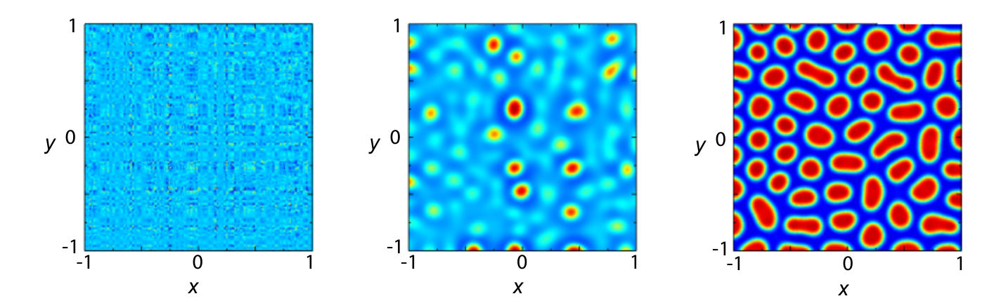
As a second example of complexity, we can consider the third definition provided regarding the concept of emergent behavior. Nonlinear reaction-diffusion systems are one of the oldest examples of systems which can show emergent behavior. The diffusion reaction system given by Eqs. (3)-(4) are known as a Turing model with Fitzhugh-Nagumo reactions; these equations represent the diffusive mixing and reaction of two chemical species (where the species concentrations are represented by the variables and ) that have the capacity to create self-organized non-homogeneous patterns in space in the steady state.
| (3) | ||||
| (4) |
In Fig. 2, the spatial distribution of is plotted for three times. At time zero (left panel), the concentration of (indicated by the color) is random in space. At the intermediate time (middle panel) one begins to observe spatial structure forming due the combination of diffusion and nonlinear reaction. Finally, at the near-steady-state condition (right panel), a spatial pattern has clearly formed showing high-concentration islands of . Although the conditions for are not plotted, they have similar initial conditions and evolution.
t]
6.3 Simplicity in Models
Simplicity when applied to modeling is not the converse of “complexity”. Model simplicity pertains to the idea that the most effective models impose only what is necessary to capture the phenomena modeled, and no more. It turns out that this idea has been around in the philosophy of science for a very long time. The idea that models should be as simple as possible has been around since at least the early 1200s (Franklin 2001). The principle is often called Occam’s razor (where razor is a fanciful terminology indicating that the idea shaves away the unnecessary) after an English Franciscan friar named William of Occam. While Occam did not originate the idea, he did make it a popular one in the philosophy of science. One version of his statement (actually appearing in his works) is given by
Plurality must never be posited without necessity
In short, the idea is this: Given two competing models for a system, each with similar predictive power, the simpler model should be preferred. Sometimes this idea is also called the principle of parsimony, for obvious reasons.
The statement of Occam’s razor has been repeated many times over the decades. Some famous examples are as follows.
- •
Isaac Newton stated in his famous text the Principia “We are to admit no more causes of natural things than such as are both true and sufficient to explain their appearances.”
- •
Einstein can be quoted as stating (in a lecture at the University of Oxford, 1933) “It can scarcely be denied that the supreme goal of all theory is to make the irreducible basic elements as simple and as few as possible without having to surrender the adequate representation of a single datum of experience.”
- •
A composer named Roger Sessions famously misquoted Einstein by stating “I also remember a remark of Albert Einstein, which certainly applies to music. [Einstein] said, in effect, that everything should be as simple as it can be but not simpler!”.
- •
A memorable version of the statement was given by Nobel-prize-winning medical researcher Theodore Woodward. His interpretation of the concept was stated by the aphorism “When you hear hoofbeats, think horses, not zebras.” While the principle was intended to be applied to diagnosis of medical conditions, it is a colorful way of summarizing the core idea of Occam’s razor.
While all of this sounds somewhat qualitative, it turns out that it can be adapted for use in a quantitative environment. In the mid 1950s a statistician named Edwin Jaynes surprised the physics community by showing that Occam’s razor, stated as the principle of maximum entropy could allow one to derive statistical mechanical results with accuracy. In conventional language, Jaynes was able to show that applying the statistical notion of maximum entropy in certain statistical mechanical computations was equivalent to inserting the minimum amount of assumptions. Jaynes was able to show that the conventional assumptions required in classical statistical mechanics could be replaced by maximizing the entropy under known constraints. Doing so would generate a solution that was maximally noncommital to unjustified assumptions. This represented somewhat of a revolution in the way that we think about modeling systems, and turned out to be very much a practical realization of Occam’s razor. Thus, what started out as a philosophical principle (Occam’s razor) turned out to have utility in a quantifiable way.
6.4 Overfitting Models
An occurrence in modeling that is related to the concept of parsimony is the problem of overfitting a model. The term overfitting comes from the related disciplines of statistics and data science. Conceptually, the idea is simple. Overfitting means to model a particular set of phenomenological data very accurately, but in a way that does not generalize well for representing other data sets of the same phenomenon. Frequently, this arises because of a lack of obeying Occam’s razor. It is easiest to explain this problem through an example.
Drag on bodies moving in fluids has been studied for hundreds of years, and frequently one finds that there is a relationship between the drag force and the square of the velocity. Suppose we run two independent sets of experiments where we measure the drag on a body in a wind tunnel for various velocities; we call these two sets of experiments A and B. We use experiment A to calibrate a model that allows us to predict the drag for a velocity. Then, we use our calibrated model from experiment A to predict the behavior of the data measured in experiment B.
In Fig. 3, we have plotted the original data (complete with a 95% confidence interval), and we have fit two different polynomials to the data. First, our experience with drag laws would suggest that a quadratic should provide a reasonable fit to the data. Our fitted quadratic (constrained to be everywhere positive) seems to match the data reasonably well, and is acceptable in that it falls within the 95% confidence interval for each data point. In Fig. 3(c), we show the results of a fifth-order polynomial (constrained to be everywhere positive) fit to the data. Including the origin, there are six data points total. It is always possible to find a polynomial of order that will go through points. Thus, the fit in this case is perfect. But is it an optimal fit? This would depend, in some ways, upon our goals. First, because we know that drag laws are generally quadratic in the velocity, a fifth-order polynomial goes against our “prior data” indicating that we might expect a quadratic form. And, while the fifth-order polynomial certainly fits the data perfectly, one has to wonder if the additional variation in the curvature represents anything physical, or is simply a very accurate representation of the experimental error that we know to be part of the experiment.
t]
One way that we can begin to answer these questions is to look to see how well this model generalizes. In other words, we have two models derived from experiment A. If these models generalize well, that means that if we take another set of experimental data (replete with its own measurement errors), the model will still provide a reasonable fit to the data (i.e., it “explains” the data). In Fig. 4 we show the results of using the models from experiment A to fit the data from experiment B. In Fig. 4(a) we show the data from experiment B, and in parts (b) and (c) we show the fits of the quadratic and fifth-order polynomial models to the data. Here, it is no longer evident that the fifth-order polynomial does a better job of fitting the data. In fact, because of the additional components of the polynomial, it actually explains the data less accurately than the quadratic model (i.e., there are two data points where the fifth-order model fails to be within the 95% confidence interval of the data points).
t]
This is a good example of the problem of overfitting. What has happened here is that we have added unnecessary degrees of freedom (i.e., additional constants and their attendant polynomial functions , , ). While these additional degrees of freedom allowed us to generate a more accurate model for a single instance of our drag data, the model failed to generalize well. This is because the model was overly specific to the data that we had. We needlessly added additional degrees of freedom to our model, in contrast with Occam’s razor. This occurred because we ignored prior data (i.e., we knew that drag models are generally quadratic). However, using the formalism of maximum entropy, we could also have looked at many such experiments, and found that the errors induced by the fifth order model were not distributed by a normal distribution (which would be expected for the quadratic fit), but rather by some skewed distribution (because it systematically under-predicts the drag in the middle off the velocity range). One can show that skewed distributions actually have less entropy than do normal distributions. In short, the more entropy a distribution has, the less parameters it takes to describe the distribution. Thus, Occam’s razor would suggest that we choose the distribution with the greatest entropy (and least assumptions), which, in this case, is the quadratic model. It is interesting that Occam’s razor has something quantitative to say about fitting models. In fact, such entropy techniques have become important tools in the burgeoning field of machine learning.
7 An Example of Model Building: Attneave’s Cat
The topic of how geometric shapes are processed by the human visual cortex has been a topic of both qualitative and quantitative research for many decades (Köhler and Held 1949), and it continues to be an active area of research for a variety of reasons ranging from the psychological (e.g., understanding the structure-function of the brain) to the practical (predicting how best to present information visually to an active user, such as in a “heads up” display).
In 1954, a psychological researcher named Fred Attneave proposed a model where he postulated that in 2-dimensional contour figures, the regions of high curvature would contain the greatest amount of information. While this theory is still being discussed in the literature (Torfs et al. 2010; De Winter and Wagemans 2008), it appears to be one component of a possibly more complex understanding of human perception and vision.
It is interesting to examine the steps in problem solving listed in Section 3 as applied to Attneave’s cat. In the following list, thoughts about each of the steps is discussed.
- 1.
Abstraction. The abstraction step involved in Attneave’s work is significant. Attneave is not attempting to model a cat, but, rather, the image of a cat. The abstraction step is the process by which Attneave asked (and attempted to answer) the question “what is it that makes an image identifiable.” In particular, Attneave was interested in stripping away everything unnecessary so that only one or two elements could be focused on. Ultimately, he chose to represent his images as a contour, with straight line segments joined by high-curvature segments. The primary output from the abstraction step in this case was the formation of the hypothesis as a relatively simple statement: regions of high curvature are the most informative in contour images. In the abstraction step, it is important to identify one’s assumptions and potentially additional or alternative variables that might be important in model revision (should that be necessary). In Attneave’s paper, this is addressed in the discussion and conclusions, where he suggests that other information (such as texture, color, contrast, and similarity) may potentially also be important, but his results were focused specifically on curvature. Identifying the simplifications imposed is an essential step in abstraction. Models are rarely completed with a single effort; more frequently, a number of iterations are needed. In order to facilitate these iterations, it is good to have a clear picture of what was included and what was left out of the model during the abstraction step. One might then revisit these variables during revision, and decided that one or more of them is needed in order to produce a models with the fidelity desired.
- 2.
Model building via an algorithmic process. The algorithm used to build the models is slightly more complex than that used simply to draw Attneave’s cat. First, Attneave wanted to test the hypothesis that curvature was indeed important. This was done by experiments with a large number of subjects who looked at simple closed curves (think potato-shapes here), where subjects were asked to place points on the curve such that they could re-draw the curve using only the points selected. From this, he was able to determine that his abstraction (segments with high curvature contain the most information) appeared to have validity. This provided good evidence from which he could generate a “model building” algorithm. Without belaboring it too much, the algorithm would look something like the following:
- (a)
For a given contour image, determine the regions of highest curvature. Attneave did not investigate the process of generating contour images themselves in detail. However, he did roughly sketch out how one might use edge detection to eliminate redundant information to determine where contours for figures might be drawn.
- (b)
Identify the highest-curvature regions of the contour figure. You may have learned in calculus that the curvature is the rate of change of the vector tangent to a curve as one translates along the curve. For plane curves, this can be expressed by
(5) While Attneave did not compute the local curvature via this method, it is not difficult to compute. In Fig. 5(a), a version of Atteneave’s cat is plotted. In Fig. 5(b) the absolute value of the curvature is plotted as the color scale along the outline of the figure known as Attneave’s cat. While this image represents the post-processed version of the contour image, it is nonetheless clear where the high-curvature regions of the figure reside.
- (c)
Keeping only the highest curvature regions in tact, replace the remainder of the components of the outline with straight-line segments connecting the endpoints of each high-curvature segment. Again, the specifics of the method were not detailed by Attneave, but one could imagine using thresholding on the local curvature as a method to decide what to keep and what to eliminate. Again, referencing Fig. 5(b), it is clear that the purple regions represent nearly zero-curvature components of the outline.
While indeed a very simple algorithm, it is nonetheless an algorithm that can be applied with little uncertainty to nearly any contour image. Some images (e.g., a circle, which has constant curvature) would be changed very little, whereas others (such as the image of the cat) would be significantly altered.
- (a)
- 3.
Concrete realization. The realization process is, literally, just “realizing” the model that has been constructed. This means after identifying the appropriate abstractions and algorithm, and then using the algorithm to take the input data (in this case, a contour outline image) to generate an output (in this case, the simplified contour outline).
- 4.
Revision. While no specific revision step is conducted in this particular modeling exercise, note that a number of important assumptions were identified by Attneave in his original (1954) paper. Attneave’s paper has been revisited many times by other researchers, and some of these have found that the neglected variables listed by Attneave were found to increase the descriptive ability of the models that they form. So, although model revision was not a component of Attneave’s model (at least, no discussion of alternative models was discussed in the paper; whether or not revisions were made in his initial work is not known), because he did describe a number of assumptions and neglected variables, other researchers have been able to extend his model to improve (to some extent) Attneave’s original model.
t]

Attneave’s cat provides a useful, and novel example of the problem solving process, with a focus on model development. It is good to think about mathematics as being only one component of problems solving and modeling. For many practical scientific and engineering problems, however, mathematics is the natural language for expressing models. A solid background in mathematics will both provide useful modeling tools, as well as experience with the problem solving process in general. Even if you never again use mathematics in problem solving (although this is hard to imagine for most scientists and engineers), the process of learning mathematics is, itself, a compelling method to practice the problem of problem solving. Problem solving skills, once learned, have considerable transferability. Learning and practicing mathematics will inevitably make you a better problem solver, regardless of the kind of problems that you are presented with.
8 Problems
- 1.
At the head of this chapter is the quote “the best model of a cat is another cat, preferably the same cat”. While the quote is somewhat humorous (and has the benefit of mentioning cats), it also has substantial meaning. In the context of thinking about systems, and abstractions of systems, write a few sentences explaining what this quote is meant to point out.
- 2.
Another quote at the start of this chapter is “all models are wrong; some are useful”. In the context of thinking about systems, and abstractions of systems, write a few sentences explaining what this quote is meant to point out. In particular, explain how it can be true that “all models are wrong”? Is there an example of any “model” that is not wrong? (Hint: refer to the quote repeated in problem 1.)
- 3.
Circles have fascinated humankind for literally thousands of years. Both the Babylonians and the Egyptians used approximations to pi, the ratio of the circumference of a circle to its diameter. But it was Archimedes of Syracuse (c.287 – c.212 BC) who really got the ball rolling (so to speak) on the topic. His idea was to inscribe regular polygons inside the circle. With increasing numbers of sides, the area of these polygons would, he posited, get closer to the area of the circumscribing circle. It is not difficult, using modern trigonometry, to show
(6)
where is the number of sides of the inscribed polygon. We can think of as being a model for the area of a circle with radius . Compute the area of a circle of for equal to 3, 4, 5, 10, 30 and 50, and compute the relative error for those values. Then answer the following questions.
-
- (a)
Does this model appear to be a sound and useful model?
- (b)
Can you show that this model converges exactly to the area of a circle as gets arbitrarily large? (Hint: for small , ).
- (c)
Suppose you had a particular application in mind where you wanted to use to estimate the area of a circle. What kinds of considerations would you need to make in order to be able to choose the value of you would use?
- (a)
- 4.
Chaotic Behavior. For certain kinds of phenomena, ranging from insect populations as a function of time to the wear rate of well-drilling bits (Li and Yorke 1975, cf.), the following model can relate the state at discrete intervals
(7) Where is a growth rate parameter, and indicates the number of the time period (each period with the same interval, say, ), and . Equations of the form (like the equation above) relate the current state of a system to the previous state. They are called difference equations; Eq. (7) in particular is sometimes called the logistics equation.
Starting in the 1960s, some researchers began to realize that such simple equations sometimes yielded surprisingly complicated (and complex in the sense described earlier in the chapter) behavior. In particular, there are values for where Eq. (7) becomes very sensitive to its initial value. This expression is so simple that it can easily be coded up in a computer language, or even computed on a spreadsheet program. Using a method of your choice, compute and plot the solutions up to given , In other words, you will need to compute a sequence of 49 values of Eq. (7) when given the first value. For the parameters and that should be used, refer to the table below.
Case x(1) r 1 0.5 1 2 0.5 2 3 0.5 3 4 0.5 3.99 5 0.5001 3.99 Table 1: Values for models using the Logistics difference equation. Once the solution is determined, compare cases 1 and 2. What is different between them. Case 3 has yet again different behavior– how would you describe the behavior in time (i.e., steps) of Case 3? Finally, note that Cases 4 and 5 are similar, except that the initial value is different by (or about 0.2% of the initial value). Do the two cases give similar or different behaviors in time?
- 5.
Models of probability. The concepts for understanding probabilistic outcomes (e.g., the result of flipping a coin or tossing a six-sided die) was one of the first physical-conceptual systems for which intensive study of via models was applied. The history of the topic indicates that improving ones odds at gambling was one of the motivations for serious study of the topic. The statistician A. Hald 2003 has stated
It was not until the beginning of the 16th century that Italian mathematicians began to discuss the odds of various outcomes of games of chance based on the fundamental idea that the possible outcomes of a single game are equally likely.
While problems in probability theory can become quite challenging, here we propose a simple system for the purposes of thinking about modeling the probabilities involved. In particular, suppose one has an urn (the urn is, for some reason, the classical reservoir supposed in such problems!) that contains three balls: one yellow, one red, and one blue. The question is: What is the probability that the yellow ball is the first one picked if one selects three balls (one at a time) from the urn.
Now, this problem is really not about computing the probabilities involved (most people’s experience would allow them to guess the probability to be without much additional thought), but to develop a model that explains the probability. While there are many different “philosophies” regarding probability, we will not dwell on that here. Instead, the following is proposed. There are three balls, and they are selected one-at-a-time from the urn. We assume that the order that the balls appear is important. There are only a finite number of possible combinations that can be selected (e.g., blue, yellow, green is one; green, yellow, blue is another that is distinct from the first example). If we assume that all outcomes of three balls are each equally likely, then enumerating all possible outcomes will allow us to answer questions about the probabilities of each outcome. For this problem, please do or answer the following.
- (a)
Enumerate each possible outcome (hint: there are 6 total possible outcomes).
- (b)
Of the total number of outcomes, how many of them represent the cases where the yellow ball is drawn first?
- (c)
What is the ratio of the number of cases where the yellow ball is drawn first to the total number of cases?
- (d)
In this model, what is the primary modeling assumption that allows us to actually compute the probabilities?
- (e)
Are there any additional assumptions regarding the process described that should be true so that the analysis is valid?
- (a)
- 6.
Consider the situation described in problem 5. Now suppose that you want to know the probability of the selecting the balls in the following order: red, blue, yellow. Can you describe the modeling process (i.e., write a short narrative) that explains how you arrived at your result?
- 7.
Consider the situation described in problem 5. Now suppose that you want to know the probability of the following result: either the red or the yellow ball is selected first. What is the probability of this outcome? Can you describe the modeling process (i.e., write a short narrative) that explains how you arrived at your result?
- 8.
Consider the situation described in problem 5. Now suppose that you want to know the probability of the following result: the first two balls selected are red and yellow, but in either order (yellow then red or red then yellow). What is the probability associated with this outcome? Can you describe the modeling process (i.e., write a short narrative) that explains how you arrived at your result?
- 9.
Consider the situation described in problem 5. Now suppose that you actually have a total of four balls: yellow, red, blue, and green. Can you use the method described for 5 to determine the probability of the yellow ball being selected first? While this method is convenient because it allows one to easily compute the probability of any possible outcome, can you see any disadvantages of this method (where each possible event is explicitly identified)?
- 10.
Describe in words as concisely and clearly as you can the problem of overfitting a data set.
- 11.
Suppose you run two experiments that show the increase in temperature at ten evenly spaced times using infrared thermometry. Your data sets are given in the Table 9.
- (a)
Start with data set number 1, and fit a line ( and a quadratic (of the form to the data set, and compute the associated coefficient of determination (also called the correlation coefficient) for both fitted curves. You can do this in most spreadsheet programs, or in a computer language. Which curve fits the data better?
- (b)
Now use the functions fitted to the previous data ( and ) to fit the data in experiment 2. Again, compute the value of for both fitted curves. Which curve fits the data better? If you were planning to generalize a model from experiment 1 to use as a fit to subsequent experiments, on the basis of what you know, which one would you choose – or ?
Time Exp. 1 Exp. 2 0 -0.110 -0.110 1 1.100 0.832 2 1.835 5.035 3 2.347 6.547 4 2.009 6.809 5 5.771 10.771 6 6.208 11.008 7 11.198 13.765 8 12.010 15.211 9 16.986 17.215 10 20.420 19.200 Table 2: Two experiments measuring temperatures. - 10.
- 12.
Information. The concept of information was brought up in the text. One way of thinking about the information content of model is to consider how difficult it is to describe. To make this concrete, think about a base-2 system of digits. Consider 5-digit integer numbers represented in base-2 format. Each such number has the form ”XXXXX” where each “X” is either a “1” or a “0”. If it is a “1”, then one sums up a unit of , where represents the numerical value of the position of the digit starting from the far right. Thus, the binary digits “10010” represent the decimal number . The information in such a set of digits is just the number of digits (which is close to the logarithm of the maximum number expressible in the system– e.g. , or approximately 5 binary digits or bits). With this in mind, please answer the following questions.
- (a)
How much information is there in the binary number 10010? How about 11111?
- (b)
Which contains more information– the binary number 11111 or the decimal number 31?
- (c)
Suppose I send a message containing a single binary digit that can be either a 1 or a 0. How much information in bits is gained by the person who receives my message?
- (d)
Consider the following two examples of a 5000 digit binary number. Case (i) each digit is generated randomly with a coin toss and written down as a 1 (heads) or 0 (tails) until 5000 digits are created. Case (ii) a number consisting of 5000 repetitions of the numeral “1”. (Hint: Can the second one be compressed some way that uses less than 5000 digits to communicate with no loss of digits? Can the first one?)
- (e)
In the answer to your previous question, does the concept of regularity of the two numbers involved make a difference in your treatment of them?
- (a)
- 13.
As briefly mentioned in this chapter, some philosophers view language itself as a model of reality. In a few sentences, describe what this might mean– that language is itself a model. Reference the discussion on the properties of models and modeling, and attempt to describe the process of abstraction, model building, realization, and revision as it might apply to a natural language by providing examples.
- 14.
Read the paper titled What is complexity science, really? by S.E. Phelan (). Phelan identifies three philosophical frameworks in which science might be defined and interpreted. What are these? Does the paper suggest that any particular framework is best?
- 15.
Read the paper titled This is not a universe: Metaphor, language, and representation by Liliane Papin (). Papin discusses some of the challenges that language poses in science. In your own words, what do you think is the main point of the paper? In other words, what is the message that Papin is attempting to communicate regarding language and science?
Chapter \thechapter Mathematical Definitions, Concepts, and Review
Almost everyone who uses this text will have some background in mathematics; it is assumed that this background includes advanced algebra, introductory calculus, linear algebra, and an introductory course in ordinary differential equations. The purpose of this chapter is to review a host of definitions, concepts about mathematics, and some of the basic results learned in previous coursework. The material presented here is not meant to be exhaustive, but is focused primarily on elements that will be useful in the remainder of the text.
Because the presentation of this chapter is specific to ideas that arise in the remainder of the text, the presentation is somewhat an agglomeration of important topics rather than an exposition focused on one or two main ideas. In a very few instances, there is the introduction of material that may not have been covered in undergraduate mathematics; for this material, however, the necessary background is only what is described in this text. Many of the topics in this chapter may be safely skipped by those who do not need a reminder about mathematical definitions, concepts, or a review of basic of linear algebra and calculus.
9 Sets and Set Builder Notation
While will not make extensive use of the concept of sets, we will use set builder notation as a convenient and compact way about discussing intervals on the real line (or higher dimensional Euclidean [sometimes called Cartesian] 2-D and 3-D spaces). The version that is adopted for this text will be simpler than is possible for more general settings. For example, there are symbolic representations for the conjunctions “and” and “or” in set builder notation; we will opt for simply using the words themselves to keep the new symbols to a minimum. The following are the elements of set builder notation that we will use. While some of these may be defined further below (e.g., the word set), here the goal is simply to describe the notation.
- 1.
Set. A set is denoted using curly braces, “”. Thus is a set containing three items, , , and .
- 2.
“Such that” symbol. In set builder notation, the colon “:” is used to indicate the concept of “such that” or “with the property that” or sometimes “as follows”. When one sees the colon after a variable (say, the variable ), it might be useful to think of this as indicating “create the set of values such that…”
- 3.
“Is an element of” symbol. We use “” as a substitute for “is an element of”. We will define element more completely below.
- 4.
“Is not an element of” symbol. We use “” as a substitute for “is not an element of”.
- 5.
Predicate. A predicate. In English grammar, is a part of a sentence that states something about the subject. In set theory, the word predicate has same notion. Thus, a predicate can be interpreted as a rule or formula that must be applied. Suppose the predicate is given by the equation (or inequality) , and we are asked to construct the set of all values of such that is met. To be concrete, let’s assume the correspondence . We could write such a set, call it , as follows
(8) This is read as follows: “create the set where is equal to the set of all numbers such that ”. There is an implication here that we know what kind of number should be. Let’s assume that is meant to be an integer. If we wanted to include this explicitly in the set statement, we could rewrite it to read the following.
(9) Here, is the special symbol reserved to indicate the set of integers.
Although we will not use them much, one can define the statement “for all” by an the statement “there exists” by . For example, the even integers greater than zero could be described in set builder notation as
| (10) |
This would be read as “create set of all values as follows: there exists values that are integers and are greater than zero. The set of values is found by taking two times the set of these values.” This concludes the number of ideas and symbols that we will adopt via set builder notation.
Now that we have the notation established, we can proceed to define some of the basic features of sets (we will be ultimately be primarily interested in the applications of set notation to intervals on the real line).
Definition 4 (Element).
An element of a set (also called a member of a set) is the generic name associated any one of the objects contained by the set. Often the symbol is used to denote the element of a set (although any symbol could be used).
Definition 5 (Set).
A set is a collection of objects; more specifically for our purposes, a collection of mathematical objects. Sets can contain a finite number of objects, or an infinite number of objects.
Definition 6 (subset).
A set where the elements of of the set are also elements of some given set. To be a proper subset, the subset must not contain all of the elements of the given set.
Definition 7 (universal set).
Many problems are created when attempting to define a completely general universal set; in the broadest sense, they can lead to paradoxes in formal set theories. For our purposes (which is primarily to discuss intervals on the real line), we adopt a universal set that is a well-defined entity that avoids such problems. Specifically, we take to be the real line in one dimension (or the 2-D plane or 3-D space in higher dimensions). One may also define to be some subset of the real line, as long as all discussions relate to intervals that are proper subsets of .
Even though our use of set theory will be minimal, it is still useful to define the basic operations of the union and intersection of sets. These are as follows.
Definition 8 (union of sets).
The union of two sets and is the set of elements belonging to either of the two sets (without repetition). This is frequently denoted by . If the elements of the sets are represented by , this can be written as . Extensions to three or more sets can be done by operating on two sets at a time iteratively.
Definition 9 (intersection of sets).
The intersection of two sets and is the set of elements belonging to both of the two sets. This is frequently denoted by . This can also be written as
Note that the concepts of union of sets and intersection of sets correspond to the English conjunctions and and or, respectively. Being explicit, the statements with implies that is in set or in set or in set (which could include any intersections among those sets). In contrast, the statement with implies that is in each of , , and .
Definition 10 (compliment of a set).
Suppose . The compliment of in universal set consists of everything in that is not in set . This is often written as (where the backslash is read as subtraction or removal). This can be alternatively written as . If defined is some subset of the real line (or higher dimensional spaces), then sometimes the compliment is called the compliment relative to .
These concepts are presented graphically in Fig. 7. One additional definition is made here, in part because it helps to clarify a notation that is often observed in the mathematical literature.
Definition 11 (Cartesian product of sets).
The Cartesian product of two sets and , is the set of all ordered pairs where and .
| (11) |
This latter notation will arise when we discuss the Euclidian plane and Euclidian space.
t] .
9.1 Numbers
The concept of numbers is a intuitive and natural thing that we have all been using since we were little and learning to count out objects on our fingers. However, numbers themselves are an interesting topic; there is even an branch of mathematics called number theory that studies the integers. While the study of integers may not sound particularly exciting, it is actually an area of intense study! For instance, number theory has been used to find very large prime numbers (numbers that are not the multiplication of two smaller numbers). Such numbers are of great value in use in public key encryption schemes an other kinds of computer security. In fact, there are several prize currently offered (of about K and as of 2021) to find a prime number with 10 or 100 million digits. The largest prime number currently known (as of January 2022) is , a number that has digits in base 10.
It turns out that the discussion of the various of sets of numbers one might encounter in applied mathematics is a good way to discuss sets and intervals in a way that has familiarity.
The most frequently used sets of numbers are as follows.
- •
– The “natural” numbers. These are the set of positive integers . Some definitions include zero; to denote that, the convention is to use the symbol .
- •
– The integers. These are the set of all positive or negative integers, including .
- •
– The rational numbers. The “” here stands for quotient, or, in other words, the ratio of two numbers. The rational numbers are formed by the set of all possible ratios of all integers and in so that all pairs for a ratio which is a member of . Note that there is a restriction; . Also, because we can have , the integers are a subset of the rational numbers.
- •
– The irrational numbers. In short, the set of all numbers that cannot be expressed as a rational number, i.e., they are not elements of .
- •
– The real numbers. The real numbers are the set of all things that we might think of as conventional numbers; in other words, it contains as subsets all of the sets of numbers defined previously. For our purposes, the real numbers can be though of most simply as the union (or the combining of) the rational and the irrational numbers (in mathematics this might be written ). The real numbers are what we use in principle when doing computations relating to physical systems. The real line can also be though of as the 1-dimensional Euclidian space, where the Euclidian spaces are defined in the next section.
- •
– The complex numbers. The complex numbers are a generalization of the concept of number that contain a real and and imaginary part. Most of us have been introduced to the idea of complex numbers early in our mathematical career; however, they frequently instill much unease and consternation. As with many mathematical constructions, however, the “reality” of complex numbers is not tremendously important. What is important is that they meet certain algebraic necessities assuring mathematical consistency (they form a commutative algebra), and, from a practical standpoint, they are useful.
A graphic indicating how these number systems (as sets) relate to one another is given in Fig. 8. Note that, for each of these number sets, the values are not part of the set of numbers! There are number sets (known as the extended reals) that contain as a value, but these sets will not be used in this text. One extension to these sets are the sets of higher-dimension Euclidian spaces; this will be discussed below.
These sets of numbers have interesting properties and histories of their own. For example, the irrational numbers were first discovered by the Greeks. In particular it is thought that a Pythagorean (i.e., a member of a Greek math cult following the tenants of Pythagoras), named Hippasus of Metapontum first proved this. Strangely, although it is the Pythagorean theorem that allowed Hippasus to show that irrational numbers exist, this went in stark contradiction to the Pythagorean belief that all mathematics could be expressed through ratios of integers. It is said that Hippasus discoverd this startling fact while at sea, and his fellow Pythagoreans were so upset by the revelation that they threw him overboard! While the validity of this story is certainly suspect, what can be said is that revolutions in the understanding of numbers has frequently been met with substantial resistance.
While many think of the complex numbers (which will be reviewed below) as presenting challenges to concrete ways of thinking, even the real numbers are a bit stranger and philosophically more challenging than one might expect. Some of the most contentious issues in defining modern mathematics has come from attempts to understand the set of real numbers, and many of these challenges arise via the subset of irrational numbers. In particular the critical notions of limits and completeness of sets, topics that we will touch on (lightly) later, that took until the 19th and 20th centuries (see Snow 2003 for more details) before the concepts were well understood. Before moving onto other topics, the following example illustrates how the concept of real numbers is more complicated than it may appear on the surface.
Example 1 ()
We have all be exposed the idea of repeating decimal numbers, but the characteristics of such numbers can be elusive. For example, consider the sequence of numbers (we will define sequences more formally in §13) that approach the value 1 as follows , or more generally . Clearly this sequence gets closer and closer to 1 as we add more repeats of the numeral 9 (i.e., increase ). Also, if we fix any small number, , then, no matter how small epsilon is, we can always take large enough so that we get closer than within to the value 1
| (12) |
In some sense, then, is equal to 1? This seems like it would be a curious thing, but we can show that it is true. The following is an informal illustration. There are proper, concrete proofs for the somewhat ad hoc illustration below. Nonetheless, the point is made, and the result is correct, as odd as the result may seem!
| (13) |
The explanation for this involves the idea of convergence of a sequence and completeness of a set to fully understand. For now, we will put this notion aside and simply recognize that real numbers (particular those that are irrational or are repeating decimals) are trickier to understand than rational numbers are! There is even some more philosophical discussion about in what sense real numbers are (objectively) real. Because of the various concepts of infinity associated with the real numbers, they sometimes illustrate behavior that is counter intuitive (the fact that is not defined is one such example; it is easy to construct examples where is equal to any number that you choose).
t]
9.2 Euclidian Space
Euclidan space might best be described, somewhat colloquially, as the 3-dimensional space that we are all familiar with. Before continuing, in order to understand Euclid’s definitions, we must first understand what an axiom is.
Definition 12 (Axiom).
An axiom is a statement about a physical or mathematical system that is assumed to be true, but cannot be proven to be true within the system itself. Sometimes axioms are called laws or principles or postulate; these alternatives names are used historically or because of disciplinary differences in terminology (e.g., between physics and mathematics).
Now we are in a position to define Euclidian space. Euclidian space is a space that we are used to thinking about in, say, ordinary geometry. Euclidian spaces subscribe to the five axioms of Euclid’s Elements. These are as follows.
- 1.
A straight line may be drawn between any two points.
- 2.
Any terminated straight line may be extended indefinitely.
- 3.
A circle may be drawn with any given point as center and any given radius.
- 4.
All right angles are equal.
- 5.
For any given point not on a given line, there is exactly one line through the point that does not meet the given line.
where the language here is not identical to that of Euclid, but the concepts are (in particular, this version of axiom 5 is known as Playfair’s axiom (Playfair 1795, p. 7)). So, why invoke Euclid at this juncture? It turns out that most of the mathematics you have done have been done in Euclidan space. In one dimension, Euclidian space is the real line; in two dimensions, the plane; and, in three dimensions what we often use as our model of space. Using set notation, in 1-, 2-, and 3-dimensions, we have
| 1-dimension | (14) | |||||
| 2-dimensions | (15) | |||||
| 3-dimensions | (16) |
Here, the Cartesian product defined above has been used in defining and .
Sometimes Euclidian geometry is also called flat space; this is to say that it has no curvature to it. Physicists (in particular A. Einstein) have shown that space is not, in fact, flat, but rather curved because of the effects of gravity. Regardless, for most systems that are terrestrial (i.e., small enough) and not subject to need for extremely accurate measurements, we may think of space as being Euclidian. What these spaces have in common is that our conventional notions of geometry (parallel lines do not intersect; all right angles are equal in angular measure) remain true in this model.
It should be noted that coordinate systems are independent of the underlying space that they describe. The conventional coordinate system that we use to describe Euclidian space is the Cartesian one, named after the French philosopher and mathematician René Descartes, who first described it. In fact, sometimes Euclidian space is called Cartesian space. However, some care is needed. A Cartesian coordinate system is the rectangular coordinate system that we are all familiar with (Fig 9(a)). The coordinate system may be a very convenient one, but it should not be conflated with Euclidian space itself. Coordinate system are a convenience in which each point may be given a unique label; but the geometry of the coordinate system does not necessarily reflect the geometry of the underlying space. For example, one may also adopt the familiar cylindrical coordinate system (Fig. 9(b)) to describe Euclidian space. This can be convenient, when, for example, one is modeling an object in Euclidian space that is itself cylindrical. While the two coordinate systems are different, the underlying space (and the geometric principles that are assumed to be true on it) remain unchanged.
While not an important concept for the material in this text, it is also possible that the underlying space itself is not flat (i.e., it is not Euclidian). For example, a spherical space is one that you may have heard of by analogy with the globe; in such a space, the five axioms of Euclidian geometry must be amended to create a consistent system. The discovery of non-Euclidian spaces (e.g., such as the spherical space just mentioned, or the hyperbolic spaces) was made in the early 1800’s by mathematicians in Europe and Russia. The discovery of such unique geometries eventually diffused into popular culture, and represented a true revolution in the way that mathematicians, scientists, and the public at large viewed science and scientific discoveries. As an example of the influence in popular culture, the ideas of non-Euclidian geometries were so widely known about that the author H. P. Lovecraft adapted the unique geometries to describe otherworldly settings in his fictional writing. As with the development of set theory (discussed very briefly at the end of the next section), the discovery of non-Euclidian geometry helped spark the revolution in mathematics that started in the early 19th century and lasting through the middle of the 20th century.
9.3 Intervals on the Real Line
The notion of an interval can be described in the language of sets, and the concept of intervals is one that we will used frequently. Below the concepts of open, closed, finite, and unbounded intervals are discussed. Analogous concepts apply for higher dimensions, but no discussion of those extensions is attempted at this juncture. Similarly, set notation is discussed, but set theory (other than the basic notion that sets exist and have elements; and we cover the basic operations of unions and intersections). It is not an overstatement to say that set theory proper forms the basic underpinning of modern mathematics. It is has also been one of the most difficult and contentious parts of mathematics, and contains controversies (or differences in approach and opinion) that are continue to generate discussion and research. While we will not go into set theory proper, or the details of why it has been such a challenging component of mathematics, we will briefly describe what gave rise to some of the difficulties at the end of this section.
Definition 13 (Interval).
An interval is a set containing all of the real numbers between two specified real numbers and ; assume that . Intervals may be open, closed, or a mixture of open and closed. A closed interval includes the end points, e.g.,
whereas an open interval does not
One curiosity about open intervals such as is that they contain a maximum or a minimum real number. By definition, the open interval does not include the end points and . Thus, for example, the open interval (1,2) contains all of the numbers greater than one, and all of the numbers less than 2, but not 1 or 2. Another way to describe an open interval, then, is as follows. For a moment, let’s consider only the minimum part of the interval specified by . Now, suppose that we select a number in the interval as close to as we like; let’s call this number . By definition, . We could then, say, select an even smaller number half way between and , and call this . This number is also in the interval because . This argument can be repeated indefinitely, and thus there is no smallest number in the open interval. A similar argument can be made for the maximum number in the open interval.
Intervals can also be half-open (or half-closed, which means the same thing) in the obvious way, e.g., is half open because the lower bound is not included. .
Finally, note that intervals can be unbounded. An unbounded interval is defined as follows.
Definition 14 (Unbounded interval).
An unbounded interval is a set containing all of the real numbers greater than or less than some specified real number, . Such intervals can be open or closed; thus is considered unbounded and closed, whereas is unbounded and open.
Accounting for various possibilities defined above for intervals (and defining the empty and degenerate intervals), then intervals of the real numbers line can be classified into eleven different types (cf. Craig 1969) listed below.
| Empty: | ||||||
| Degenerate: | ||||||
| Proper and bounded: | ||||||
| Open: | ||||||
| Closed: | ||||||
| Left-closed, right-open: | ||||||
| Left-open, right-closed: | ||||||
| Left-bounded and right-unbounded: | ||||||
| Left-open: | ||||||
| Left-closed: | ||||||
| Left-unbounded and right-bounded: | ||||||
| Right-open: | ||||||
| Right-closed: | ||||||
| Unbounded at both ends (both open and closed): | ||||||
This last interval (the real line) is listed as both open and closed. This is a technical detail that creates no end of discussion on mathematics forums on the internet. The explanation is not easy without invoking additional mathematical structure (such as topology). In short, however, it might be described something like this: The real line contains all possible real numbers; thus is it closed with respect to the real numbers. However, there is no maximum nor minimum real number on the real line, thus (as for the discussion of the open interval) the real line is also open. While this sounds like a paradox, it is also a statement that binary options (“true” or “false”) in mathematics are not always necessary; sometimes there is a third option which is “neither true nor false”. There is a saying in mathematics that “A door must be either open or closed, and cannot be both, while a set can be open, or closed, or both, or neither!” (Munkres 2014, p. 91). While this may sound a bit noncommittal, the reality is that these concepts are both well defined and useful.
A short note about set theory. We have used set notation above, but not invoked set theory per se. You may have learned a little about set theory even in grade school – the ideas at that level are usually to discuss how one might group objects together (creating a set), and then compare the properties of various sets. On the surface, this seems deceptively simple. However, the goal of developing a robust set theory led to one of the most interesting periods of mathematical research in the history of mathematics. By robust here, something specific is meant. This means that the theory must propose sufficient axioms such that it is both complete and consistent. The word complete in this context means essentially that “every true statement in the system can be proven from the axioms”. The word consistent means essentially “every proper statement (or question if you prefer) within the system can be shown to be either true or false.” The hope was that because set theory was so fundamental, then, in principle at least, a powerful enough version of set theory could be the basis for deriving all of mathematics (at least, in principle). Quite unexpectedly, such a set theory was ultimately proven to be impossible.
Early work on set theory was done by many mathematicians; but in particular the work by two German mathematicians – Richard Dedekind and George Cantor – from about 1870 to 1900 paved the way for what is sometimes referred to as Naive set theory. A good and short introduction to this history can be found in (Ferreirós 2022). The modifier “naive” here is not a slight; it means only that the theory was not cast in the language of formal logic. While this set theory was incredibly useful, Cantor was alarmed to find that it was not consistent – in other words, he found that paradoxes could be constructed in the theory. Without recounting the entire history of set theory, the inability to generate a paradox-free set theory led to a crisis in mathematics in the early 1900’s. This crisis, while long in the making, was made most apparent by Bertrand Russel who described the paradox in 1901. The Russel paradox is a mathematical statement much like the so-called liar’s paradox, which make the conflicting and self-referential statement “This sentence is not true”.
This kind of paradox would have deep and lasting ramifications for mathematics. While set theory was ultimately repaired to some degree by the mathematicians Ernst Zermelo and Abraham Fraenkel in the 1920s (known in mathematics as the ZFC set theory). The statement “to some degree” must be qualified here. The ZFC avoids the kinds of paradoxes that plagued earlier versions of set theory. However, in the 1930s a mathematician named Kurt Godël proved a rather unexpected result. Gödel was able to show, roughly, the following: Any axiomatic system which is complex enough to describe ordinary integer arithmetic is either incomplete or inconsistent. In other words, if our axioms are consistent (i.e., do not lead to paradoxical or undecidable statements), then in every model of the axioms there is a statement which is true but not provable. While this result was somewhat of a blow to the idea of generating an overarching theory for mathematics, the actual impact is still debated. First of all, the proof used by Gödel was of a particular flavor known as first order logic. Thus, it is unclear if more capable logic languages suffer the same fate. Secondly, while the premier set theory, ZFC, must by Gödel’s theorems either be inconsistent or have true but unprovable statements, it is not clear that this has any practical import. For example, if I state “all non-pterodactyls are not non-dinosaurs”, I have certainly uttered something true. Regardless, if I am not interested in anything about dinosaurs (flying or not), then this true sentence is of no value to me. So, while it might be impossible to prove all true statements in ZFC, so far the such unreachable truths have not created any practical problems (possibly because, like the example, they convey truths that are not relevant). And, to date, nobody has found an inconsistent statement within the context of ZFC. Thus, ZFC has been a useful tool in mathematics. The search for more powerful set theories continues as a topic of interest in mathematical research.
9.4 Complex Numbers
Unlike, say, the natural numbers (which can be illustrated by collecting actual objects), the complex numbers are a purely mathematical construct. That does not mean that they are not useful or interesting, however. There are many examples of concepts that exist only mathematically, but are nonetheless useful for many practical applications.
The complex numbers are an extension of the real numbers. Although almost everyone reading this text has probably encountered them previously, it is useful to recap their basic properties.
Definition 15.
A complex number assumes that there exists a mathematical object, called the unit imaginary number, , such that so that . Every complex number consists of two parts, a real part, and an imaginary part that is proportional to . The conventional form for a complex number is , where and are real numbers. The set of all complex numbers is usually denoted by .
The rules for addition, subtraction, and multiplication are slightly modified from those of real numbers as follows. First, addition and subtraction are done by adding and/or subtracting the real and imaginary parts of a complex number independently. Therefore
Multiplication of two complex numbers is defined as follows
or, equivalently, grouping terms
The complex numbers are often represented as vectors on a plane, where the real part is plotted on the horizontal axis, and the complex part on the vertical axis. In this representation, a complex number would be represented by a pair of points, i.e., . There are some advantages and disadvantages of this, but it generally improves interpretation for problems with physical significance. When this formalism is adopted, a complex number is frequently represented typographically as a vector, as in . The representation of the complex numbers in this manner requires mildly re-defining the vector dot product. We define this in the following.
Definition 16 (The Complex Conjugate).
For a complex number , the complex conjugate is defined by .
Definition 17 (The Complex Dot Product).
For two vectors and , the complex dot product between and is given by
which has the advantage of being a single real number. In particular, this means that a vector dotted with itself is defined by
and the magnitude of a complex vector is defined by a rule that looks much like the rule for computing the length of a vector on a plane
t]

The recognition that complex numbers can be treated as vectors on a plane implies that they can be conveniently represented in polar coordinates. In fact, there are some significant reasons for doing so. To start, define the length of the vector by the number . Then, we have the following relationships between the and coordinate systems (Fig. 10)
| (17) | ||||||||
| (18) | ||||||||
or,
| (19) |
In this representation, is sometimes called the magnitude or modulus or absolute value of the complex number, and is called the argument of the complex number.
You may have seen Euler’s formula before; it is the formula that leads to the famous relationship (where, recall, is the base for the natural logarithm). More generally, however, Euler’s formula takes the form
| (20) |
Although this formula looks truly remarkable, once we accept that the imaginary numbers are an acceptable extension of the reals, the proof of this result becomes quite simple (we will examine that further when we tackle infinite series). For now, we adopt the formula without proof. However, note that it allows a particularly simple representation of a complex number as given by Eq. ((19)) in the form
| (21) |
As an interesting side note, this last formula allows one to make sense of the logarithm of a complex number. Taking the natural logarithm of both sides of Eq. 21, we have
| (22) | ||||
| (23) |
Noting that , then it is clear that there are generally an infinite number of representations for the logarithm of a complex number
| (24) |
Although complex numbers have a helpful representation as vector quantities on the complex plan, they are technically just an extension of the real number system. Therefore, it is not common to adopt a bold-face type to represent them (as we have done above). In general, complex numbers are set in regular, italicized script, (e.g., ). Generally, the context prevents there from being any confusion. In future uses of complex numbers, we will not use bold-faced script to represent them. Thus, the equation above would be more properly written
| (25) |
10 Functions
We all have been introduced to the concept of functions. When most people in college mathematics think of a function, the first thing that comes to mind is a relationship that looks something like
| (26) |
In this description, we are given a domain (the numbers such that - recall, square brackets indicate inclusive interval notation), and a range for the function (the values for the defined domain). A graph of this function is plotted in Fig. 11. Although this is how we typically think of a function, we can define it more generally.
t]
Definition 18.
A function (or sometimes mapping) is a relationship between two sets, and , such that each element of is uniquely associated with an element of .
The word uniquely appearing in our definition here is really important: a function is always single-valued.
This definition requires a bit of additional explanation for our purposes. First of all, for us, the sets involved for a function are almost always intervals of the real number line. We even give these functions additional names and descriptions, as follows. We usually refer to functions as having independent and dependent variables. The independent variables are the inputs to the function (or more properly, the set that is input to the function; this is the set in the definition). Conversely, the dependent variables are the set of values that are produced by the set of independent variables upon application of the function (this is the set in the definition). Each member of the set of independent variables is mapped to exactly one member of the set of independent variables (this is the uniquely part of the definition). Fig. 12 gives a pictorial representation of the process.
t]
The concept of functions that strictly increase or decrease is one that is used routinely in mathematics; so much so that they have a special name: monotonic. These functions are defined as follows.
Definition 19.
A function is said to be monotonically increasing on and interval, , if the following are true:
- 1.
for all in .
- 2.
is not the constant function (, a constant).
Similarly, a function is said to be monotonically decreasing if the following are true:
- 1.
for all in .
- 2.
is not the constant function.
Obviously, functions in general are neither monotonically increasing nor decreasing, but a combination of these two concepts over subdomains of their total domain. The constant function is neither monotonically increasing nor monotonically decreasing on any subdomain of its domain.
There is one final class of functions that requires definition because the term arises so frequently in applied mathematics. These are the algebraically homogeneous, or simply homogeneous, functions. Note that later on, the concept of homogeneous differential equations will be discussed; while the concepts are related, one should not confuse the two. Here, we define algebraically homogeneous functions as follows:
Definition 20 ((Algebraically) homogeneous function).
An algebraically homogeneous function is one with multiplicative scaling behaviour: if all its arguments are multiplied by some factor, , then the effect on the function is that its value is multiplied by some power of the factor . In other words, homogeneous functions display the following behavior
Here, is a real number, and it called the degree of the function.
Example 2 (Homogenous functions.)
Below are a few examples of homogeneous functions.
- 1.
All polynomials of the form are homogeneous. To see this, just note the following: . In this case, the degree of the function is equal to the degree of the polynomial.
- 2.
No functions with additive constants are homogeneous. This is also easy to demonstrate. Suppose is a homogeneous function. Now consider the function . The function cannot be homogeneous, because a multiplicative scalar will not scale the constant . Functions like (i.e., ones that contain an additive constant) are called affine. This just means that the two functions are connected by a linear scaling of the coordinate (the independent variable) followed by a translation (the additive scalar).
- 3.
The function is homogeneous. To see this, note
So, this function is homogeneous, with degree equal to .
10.1 Boundedness
In science and engineering, we usually think of the sets involved as being intervals of the real number line. To put this in context, think of our example given by Eq. (26) above. Here, we can define of the input set in set builder notation as (as a refresher, this is read as follows: “The set A is constructed by collecting the all of the numbers such that is between -2 and 2, inclusive of the endpoints”). The set we can think of as all of the numbers defined by the function . Recall, we have . The output set, , is defined by . Note also that these intervals are either or intervals. The concepts of and intervals (or, generally, sets) is actually much deeper and complex than one would assume (as described in §9.3. Now, we combine the ideas of intervals of independent variables, and functions on those intervals. The following is an example.
Example 3 (Domains of a Function as an Interval)
The function
| (27) |
has the domain . The function is monotonically decreasing on this domain. While the function may not seem particularly unusual, it actually does have some strange behavior at . A plot of the function is given in the figure below.
This function is perfectly well-defined all all points between and (that is, ), but it is undefined at . One difficult concept arises in this kind of description, and this is encountered when you ask the following question: What is the minimum value of the set forming the domain? Technically, the domain of this function has no minimum value! The number is not in the domain (hence, the “(” in the domain description). However, for any small number , say , the value of the function is very near 1. It is only undefined at exactly . In cases like this, where we can’t technically use maximum or minimum, we say instead that the number 0 is the greatest lower bound or infimum of the domain. Here, one needs to interpret “greatest” as follows: of all of the lower bounds for for the interval where is defined, is the largest of them. Any larger value would be within the domain, and is thus not a bound.
The example above suggests that identifying the smallest number in an open set is not generally possible. However, one can often identify the largest number that forms a lower bound for the set (in the example above, this is the number 0). This leads to the following theorem (which we will not prove!), which we will use primarily as a definition.
Theorem 10.1 (Least Upper Bound, Greatest Lower Bound)
If an interval has any lower bound, then it also has a greatest lower bound (g.l.b., or infimum). That is to say, there is a unique number, , which is a lower bound for the interval such no larger numbers are lower bounds. Any numbers larger than are either (i) in the interval, or (ii) greater than or equal to an upper bound of the interval.
A similar statement can be made about the upper bound. If an interval has any upper bound, then it also has a lease upper bound (l.u.b, or supremum). The least upper bound is a unique number, , which is an upper bound for the interval such no smaller numbers are upper bounds.
To help make this more concrete, consider the interval we examined above: . For this interval, the greatest lower bound is the number 0, even though the number 0 is not in the interval itself. The least upper bound is the number 1. No numbers, , smaller than 1 are, obviously, upper bounds for the interval, because and 1 is in the interval by definition.
Many of the functions that we encounter in applications are mappings that never tend toward infinite values. In part, this is because physical systems never really have phenomena with infinite magnitude. However, in many instances it can be useful model a phenomenon as if it tended towards infinite value. Additionally, some purely mathematical concepts require the definition of functions that tend toward infinity (e.g., the tangent function, , necessarily tends toward infinity as tends toward zero). It is useful to establish the concept of functions being bounded (and, hence, also being unbounded) as a matter of the vocabulary used in mathematics.
Definition 21.
A function, , is bounded on some interval if there is some number, such that for all .
Any function that is not bounded is unbounded. An example of a bounded and unbounded function appears in Fig. 14. In this figure, part (a) contains a bounded function. The gray dashed line in the figure represents the absolute value of the function. The horizontal line at indicates the minimum value of that bounds the function. All values of the absolute value of the function are less than or equal to , thus the function is bounded. Note, in general there is no need to establish the minimum value of , as done here, to establish the boundedness of the function. Had the choice been , it would still be possible to show that all valued of the function are less than , and the function is therefore bounded. In Fig. 14(b), an the function function is plotted. This function is unbounded on this interval as . For every choice of , we can always find a value of sufficiently close to 1 such that the value of is larger than . Thus, even though the interval of definition does not contain the value of 1 (in which case one would find an infinity defined by ; this is sometimes called a singularity), the function is still unbounded! Note that while we often think of an unbounded function like having a value of infinity at the singularity, it is more proper to think of the function as being undefined at the point . The reason for this is the following: up to the point , we can imagine a limiting behavior that is well defined. In other words, it is correct to say
| (28) |
because it indicates the limit of numbers that take the form , where is any real number less than 1. The ratio is always defined, because is never equal to 1 in the interval defined. This is in contrast to setting ; in this case, the function evaluates to . The form is not “infinity” as it is sometimes (incorrectly) represented. Technically, the expression has no definition at all; it is an undefined operation. While this last discussion is perhaps a bit overly-technical, there are a number of examples in applied mathematics where this seemingly technical point is enormously important in generating the proper understanding of a problem.
t]
10.2 Continuity
Functions are not necessarily always continuous. For example, consider the following function. Assuming , define the function
| (29) |
t]
This function is plotted in Fig. 15. Although it is true that this function requires some extra handling (for the point ), the end result is not too dissimilar to what we are used to seeing. However, it does indicate that it might be useful to further characterize functions on the basis of how continuous and smooth they are. A few comments about the various labels that are applied to functions to describe how smooth they are are provided in the following.
A function is continuous if it changes gradually as the independent variable changes. For a one-dimensional function, one can think of this as being able to draw the function with pen and paper without taking one’s pen off the paper. More formally, using the dreaded - arguments, one make a more concrete statement. Unlike most - arguments, we are going to do this in slow steps. First, suppose we are interested in the continuity of a function at a point . Now, we look at all of the points within a small distance, , around . We can denote those points by all of the values for such that , or, equivalently . Now, for all of such points that we find on the axis (the domain), we can compute the absolute value . Suppose we do this, and we find that there is a number such that
| (30) |
Now, for a continuous function, we expect that as we squeeze the interval by making smaller, we should also be able to correspondingly find a new value for that meets the criterion given in (30). In other words, as gets smaller, so does . This is essentially the way that continuity of a function is defined. Formally, the argument is turned inside-out (which is common in the presentation of definitions and proofs in mathematics…), to read as follows
Definition 22.
A function, , is continuous at a point if and only if (i) is in an open interval of the domain of , and (ii) we can always pick an (as small as we like), and still always find some interval around (that is, ) such that , regardless of how small we have chosen to be.
Definition 23 (Continuous Functions).
A function is continuous on and interval, , if it is continuous for each open sub-interval of .
In essence, the “for each open sub-interval” part of the definition is to avoid any possible problems with defining continuity at the least upper or greatest lower bound of the interval. In short, we don’t need to worry about continuity at the end points of our domain. This is designed specifically to avoid potential ambiguities as were discussed for the function in Section 10.1.
These definitions can be a bit tricky to apply, and they are not the only way to define continuity. Alternatively, one can insist that the following limits, taken from the left and right sides of must be valid for each point in a domain for a function to be considered continuous.
| (31) | ||||
| (32) |
And sometimes this alternative is easier to use in applications. Note. The long double arrow () in mathematics should be interpreted as meaning “this implies”.
Regardless of which method is used, the results are the same. This is easiest to see with a simple example, as illustrated in Fig. 16.
Example 4 (Continuity of Functions)
In Fig. 16, it is apparent from inspection that the function (the orange line on the Fig. 16) is continuous. Suppose we consider the point . Clearly, we can pick a small number, say , such that there is a small enough interval around () where . In fact, we can compute what this interval is as follows
| Accounting for the absolute value, there are two options | ||||||
| Solving these inequalities for , we find | ||||||
| The first of these is the smallest, so it is safe to take equal to that value. | ||||||
You can check this directly by noting that
No matter how small we make , we can always find a value of so that the inequality is valid.
Now consider the function (the blue line on Fig. 16). Here, our scheme works reasonably well until we set to be less than about . Because there is a jump of right at , we can easily find an that breaks our definition. For example, set . Now we are looking for the values of in an interval , such that . Of course, we can see just by looking at the graph that there is no such interval. In any small interval around , the value of is at least , but definitely never smaller than that value.
The definition of continuous, then, aligns with our intuitive notion, even if the definition itself takes a bit of thinking to fully understand.
t]
Functions that have a jump in them, such as the one in Fig. 16 are called discontinuous. When there are a finite number of discontinuities, sometimes the functions are called piecewise continuous. In other words, a piecewise continuous function is a function that has a finite number of jumps in it and doesn’t blow up to anywhere. This is an important enough concept that it deserves a specific definition.
Definition 24 (Piecewise Continuous Function).
A piecewise continuous function is a function that is at continuous everywhere, except at a finite number of points.
Within continuous functions, the functions are sometimes by their derivatives. As an example, examine Fig. 17. This function is defined by
| (33) |
t]
In general, the word smooth is used to indicate a function that has a derivative at each point in its domain. Thus, the function given by Eq. (26) is smooth; the function given by Eq. (29) is technically non-smooth, but this arises because of the discontinuity imposed by a single point. Extending the idea of piecewise functions, we can call the function given by Eq. (36) piecewise smooth. Most of the functions that we study in this text will be of this kind.
Definition 25 (Piecewise Smooth Function).
A piecewise smooth function is a function where the first derivative of the function is well-defined (i.e., it exists, and it is not infinite) everywhere, except at a finite number of points.
We can further characterize smoothness by how many derivatives a function has. If a function has an infinite number of derivatives that exist, then it is called . An example here is the function . This function is smooth (it is plotted in Fig. 18), and is often called a Gaussian function. We can define particular functions that are called analytic functions; however this will have to wait until after the review of derivatives and integration is presented.
t]
Some functions have only a limited number of derivatives that exist. As an example here, consider the function
| (34) |
This function looks innocuous enough- it is plotted as the orange curve in Fig.19. However, its derivative (plotted in blue) has a cusp in it at the location . Therefore, although its first derivative exists and is continuous, its second derivative is not defined at . To reflect this, functions with one continuous derivative are called . Although we have not yet reviewed derivatives, we note the following generalization of this idea.
Definition 26 (-order continuous function).
Suppose a function is such that the first derivatives (i.e., , , ) are both bounded and exist (i.e., there are no points such that the derivative of order generates a cusp or other discontinuity). Then the function is continuous in the derivative up to order , or, more simiply, .
t]
There is a special class of functions called analytic that have a number of interesting properties. Many of the familiar functions that we know about are analytic. Examples include
- 1.
All polynomials of finite degree.
- 2.
The exponential and logarithmic functions.
- 3.
The trigonometric functions.
In the early days of mathematical evolution (say, through the early 1900s), analytic functions were synonymous with functions. Since that time, the notion of what constitutes a function has grown considerably; some of the unusual examples of functions that are not analytic in some part of their domain (or everywhere, in the case of the Thomae function given in Fig. 21) are presented in the material later in the text.
Definition 27 (Analytic Function– Definition 1).
Suppose a function is defined on a domain, . The function is analytic function everywhere in if for every closed interval that is a subset of () there exists a constant such that for every point and every non-negative integer, , the following bound holds
| (35) |
While this definition does make a mathematical mouthful, it is relatively easy to understand intuitively. What the definition is trying to tell us is that, for any closed finite interval that is part of the domain of the function, that the function, nor any of its derivatives, go to infinity in that domain. There are some technical issues regarding the domain of the function (and the closed subsets that are selected from it) that will not be covered here. In general, however, we can think of a function as being analytic at a point in its domain if its value and the value of all of its derivatives do not tend toward infinity.
As a final note about the classification of functions, there is one additional classification that is useful to know about. There are, in one sense, two different kinds of functions that we use in common practice. There are polynomial functions, and the roots of polynomial functions to start with. A polynomial function is a polynomial (of any finite order) whose coefficients are also polynomials. For example, a polynomial function of order 4 is defined by
For such a function, the roots generate new functions, , involving (rational) fractional powers (including negative powers). Such functions are called algebraic because they can be defined using only the rules of algebra applied in a finite algorithm. The following are all examples of algebraic functions.
The nice thing about these functions is that they can be entirely described mathematically simply by describing the polynomial that generates them. Algebraic functions are expressions involving only a finite number of terms, and using only the algebraic operations addition, subtraction, multiplication, division, and raising to a rational fractional power. In a sense, we fully “understand” these functions as long as we understand the operations that define them. This is literally constructive- for many examples of algebraic functions, we can give someone an algorithm (with a finite number of terms) that explains what the function is and how to compute its values. Importantly, all algebraic functions are given by the roots of some polynomial; however, for rational polynomials of degree 5 or higher, it is not true that all such polynomials have roots that are algebraic functions (the proof of this is known as the Abel–Ruffini theorem).
It turns out, however, that there are many interesting and useful functions that are not the roots of any polynomial equation. Familiar examples include the , , , and functions. Such functions are called (and, yes, this is really the name) transcendental functions. The idea behind the name is that these functions transcend description by the discipline that we normally call algebra. Transcendental functions will show up later in our studies of differential equations, and some will prove to be essential for describing solutions to such equations. All transcendental functions are analytic (a term we will define in by the Taylor series in detail later), so they all have convergent Taylor series representations.
There are functions that are even more …interesting to attempt to defined because their structure begins to challenge the concept of function altogether. Consider the following function (sometimes called the modified Dirichlet function or the Thomae function)
| (36) |
It is understood here that is expressed in fully reduced fraction form. This is a really unusual function, and clearly it has no simple, closed algebraic formula. A plot of this function appears as Fig. 16. In addition to its strange definition and look, it also has some other unusual characteristics. It turns out that the real numbers are “denser” than the rational numbers. In a sense, there are more (many, many more) irrational numbers than rational ones. Thus, this function is continuous (and has a derivative) at each point where is an irrational number. It is discontinuous at every point where is rational. It is not terribly important to understand from this example all of the details of why this kind of behavior exists (although our discussion of intervals above is suggestive), but the essential idea is to build an intuition that the real (irrational) numbers constitute a much larger (denser) set than the rational numbers do.
10.3 Equivalence Classes of Functions
Later on, when we discuss the concept of Fourier series, it will be helpful to understand the notion of equivalence classes of functions. In short, two functions and are considered to belong to the same equivalence class if they differ from each other by, at most, a finitely countable number of points. An example of two functions that are of the same equivalence class is given in Fig. 20. The mathematical representation of these two functions is given by
Note that we have the following limits for (the function on the right-hand side) near
where indicates the limit coming from the right-hand side, and represents the limit coming from the left-hand side. Be sure to recall here that the limit exists in the sense of approaching the value , but not actually reaching that value. If you need a refresher on one-sided limits, your undergraduate calculus text will definitely cover this material.
t]
It turns out that, from the perspective of integration (including Riemann integration– see §12.3), the presence of a single discontinuous point does not affect the result of the integration. Speaking colloquially, a single point has no measure, so it does not add or subtract from the integral. The following definitions makes this more formal.
Definition 28 (Removable discontinuity).
A function is said to have a set of removable discontinuities if (a) the number of discontinuous points is finite, and (b) the left and right-hand limits at each point of discontinuity are equal. The value of the function at the discontinuous points can be taken to be the value of the limit at that point.
Definition 29 (Equivalence class of functions).
Two functions and are said to belong to the same equivalence class if (a) the two functions and have only removable discontinuities, and (b) =0 for all points that are not located at a discontinuity in either or in . Alternatively, (b) could be stated by “ after all discontinuities are removed”.
t]
11 Linear Spaces, Linear Operators, and Linear Algebra
We will have only a few occasions to use linear algebra in this material, but it is worth briefly reviewing, and it also allows us to discuss the concept of an linear operator. Many of the problems that we encounter in the material to come involve linear operators, so spending some time understanding what they are is worthwhile.
Operators are just what they sounds like: They are mathematical constructs that operate on something (say, a function) to generate something else (for example, a different function) (Fig. 12). This is a very general concept, and it is difficult to give it a precise meaning. As an example, all functions are operators. To make this concrete, take a look at the following example.
Example 5 (Functions as operators.)
We are all familiar with the idea of a function. In the notation that we have are probably most familiar with, a function is defined as a one-to-one (i.e., unique) mapping between two sets. In a more familiar setting, we think of a function as having a range (which is usually an interval on the real line, plotted on the horizontal axis by convention) and a domain (which is usually some portion of the real line, plotted on the vertical axis by convention). For example, a properly defined function would be any of the following:
| (37) | ||||||
| (38) | ||||||
| (39) |
These functions are plotted in Fig. 22.
What is important to realize about these functions is that they are operations on their independent variables. In some sense, a function exists separately from their independent variables. Thus, once I have defined, , as, for example, in Eq. (37), then what I have really done is to define an operation to be performed on one set (the independent variables) to generate another set (the functional value). Often when we think of functions as being operators, we consider (1) the function to define the operation, and (2) the operation is done on whatever is put into the function. The thing put into the function, when used in this sense, is often called the argument. The argument can be a simple independent variable defined over an interval (our conventional use of functions) or some other set.
For example, suppose we define the following set: . We would read this in words as ”The set is the set that contains values of such that is equal any of the values 1, 3, 4, 5, and 42”. The set has a finite number of values in it, but we can still use any of the functions above as operations on this set. Let’s interpret the following way:
| or, computing the values using the expression | ||||
We can even think about putting functions in other functions (creating a as arguments when we use the operator idea. As an example, consider the function . Now, can we make sense of the operations and ? Sure, we need only apply the operations to the argument of the function, regardless of what the argument is.
When we interpret a function this way, we sometimes write the function without the independent variable (with the idea that the independent variable can be anything), as in simply . This is just a notational device used to be more compact, there is usually no deeper meaning associated with it.
11.1 Linear Operators
Now that we understand the basic idea of an operator, we can consider what a linear operator is. This is actually pretty simple at this point.
Definition 30 (Linear Operator).
A linear operator, , is an operator that subscribes to the properties of additivity and homogeneity. Specifically, this means
| (40) | ||||
| (41) |
Linear operators are a subset of all possible operators. In fact, most interesting phenomena in engineering and physics are nonlinear in general. Linearity exists only as an approximation to the more general nonlinear behavior. In this text, we will be generally concerned with (although not exclusively!) linear operations and linear operators.
As discussed above, functions can themselves be though of as operators. Thus, a linear function would subscribe to the properties of additivity and homogeneity above. As and example, the following function is linear
| (42) |
To show that it is linear, note that we can prove both additivity and homogeneity in one step. If we make the substitution , then we find
| (43) |
illustrating that the function is indeed linear.
There is a particular feature of linearity that can create some confusion. We are used to calling functions such as linear. However, it is not difficult to show that this function does not meet the properties of additivity and homogeneity (try it!). There is a subtle reason for this failure. In a very real sense, is actually the translation of a more fundamental function . Take a look at Fig. 23. Each of the functions illustrated is a translation of the function . Such translations are called affine transformations. It turns out that when we call a function linear, we actually mean that the fundamental function itself (where ) is linear. The constant term only represents an affine transformation of this more fundamental function. In fact, in each of the lines defined in Fig. 23, we could eliminate the constant term by simply making a transformation of the coordinate system. For example, if we moved the coordinate system vertically by a distance of 2, then the blue line in the figure would then have . Thus, in a sense, all affine transformations of a function are the same as far as linearity is concerned. In order to assess linearity, the first step would be to first make an affine transformation of the coordinate system so that . In a more practical sense, we can essentially ignore constants when checking operators (including functions) for linearity.
t]
Example 6 (A familiar example: The derivative as an operation.)
The process of differentiation is one example of a familiar operation. Consider, for example, the following.
In this example, the operator is defined by derivative notation, . When we say , we are just defining the fact that the “abstract” operator in this case is the derivative operation, denoted by .
Example 7 (The derivative as a linear operator.)
Is the derivative operator a linear one? We can check. Recall the definition.
| (44) |
Since our operator in this case is just , we need only to check that the linearity identity is met. In other words, we need to evaluate
This is exactly the form that a linear operation must take as defined by Eq. (44), so the derivative is a linear operator.
A compound linear operator is just the sum or one or more linear operators. The easiest way to understand these is through some simple examples. Although we will not use operator notation extensively in this text, it is a useful notation to understand.
Example 8 (Compound linear operators)
Compound linear operators act as follows.
| (45) |
It is important to recognize that, although the notation looks as though it indicates multiplication, it does not! Here is a more complex looking example that helps to understand the idea better.
Note that the operators do not act like multiplication!
Functions can be treated as operators also; but only homogeneous functions are linear operators.
Example 9 (Functions as operators.)
Consider the functions defined in the previous example.
| (46) | ||||||
| (47) | ||||||
| (48) |
Are they linear operators? To check this, we need only try the operations on the quantity to see if the conditions given by Eqs. (40)-(41) are met. For the generic operator , we will substitute our particular functional operators. Thus, for the example of , we have the result
Which indicates that is linear. For the function , we find
so is not a linear operator (and also not a linear function!). The final function is left to the reader to check.
There are two more concepts that are useful to introduce when discussing the (somewhat abstract) concept of linear operators. These are the identity operator and the inverse operator.
Definition 31 (Identity operator).
The identity operator, , is any operator such that for all admissible objects in the domain of (e.g., numbers, functions, vectors, etc.) .
Example 10 (Identity operators.)
Here are three common examples of identity operators that you have seen before.
- 1.
The number “1” is the identity operator in arithmetic. For any number , we have .
- 2.
We can define an identity function in a domain as follows: for all in . It is not too difficult to recognize that this operator is equivalent to multiplying a function by the number 1.
- 3.
consider the following matrix multiplication (Note: linear algebra is covered in the next section).
Now, for every possible vector of dimension two, we have
Therefore, is an identity operator for the domain of vectors of dimension two.
We won’t be using the theorem-proof format very often in this material, but occasionally it is helpful, especially when the proofs are short and clever. The definition of the inverse operator can be done this way.
Theorem 11.1 (Inverse operator)
A linear operator can have an inverse, , only if implies that .
Proof.
If then the inverse of is the mapping which takes back to . (AN ASIDE: Here, it might be helpful to think of a conventional function, such that , and is the domain of the horizontal axis. For example, associates each independent value in the domain with a unique value for the result (which we call ) in the range.)
Suppose now that and . Then by linearity . One of the following results must be true, either (a) (i.e., and are the same value), or (b) , so that two values of in the domain of that would be mapped to the same value in the range. For the inverse function, the roles of the domain and range are interchanged. Thus, for the inverse function, forms the domain, and is the range. However, by definition, a function can have only one value in the range associated with a value in the domain. Thus, the option where and are not equal is not possible (or the inverse would not be a function). Thus we must have that , and this means is only true for . ∎
Without getting overly-technical, for our purposes an inverse linear operator will exist when we can show
| (49) |
and that is never multiple-valued.
As usual, examples can really help make these ideas more clear. {svgraybox}
Example 11 (Inverse operators.)
- 1.
Suppose we have for . Does this function have an inverse?
Try these functions
(50) (51) Now, note that . But, from Eq. (50), we have ; thus, we have . Now, note that the identity operator is such that . So, by definition, we must have that . Therefore, is the identity operator, and, by definition, is the inverse of .
Functions that are inverses of one another have an interesting graphical feature. Consider the two functions above; if we plot them both as functions of (i.e., we plot the functions and , we obtain the plot below. Functions that are inverses of one another have reflective symmetry about the line .
Figure 24: Inverse functions.
There is one caveat that needs to be attended to when discussing the idea of linear operators and linear equations. The idea of linearity is usually associated with only the operator part of the equation. In particular, what this means is that constants involved in a function are excluded. This is by convention, not necessity. Consider the following linear equation.
| (52) |
Obviously the operator must be linear, because is a line! However, if we attempt our normal process for checking linearity, we encounter a problem
| (53) | |||||
| (54) | |||||
So, what went wrong? Well, the answer here is a bit tricky. We should, technically, think of constants as not being part of the operator. In other words, suppose we define . Then, the equation above can be written
| (55) |
And the actual question can be posed as “is the operator linear”? And the answer to that question is obviously yes. The important thing to remember here is that the linearity of the equation has only to do with the operators involved, not with any particular constants that may be tacked on to the operators. Thus, a linear equation is any equation whose operator (which, by definition does not include additive constants) is linear.
11.2 Linear Algebra
Now that we know what a linear operator is, we can discuss linear algebra. Most people’s experience with linear algebra leaves them without an intuitive notion of what is really going on. Because linear algebra is such a mathematically rich topic– it is the first place where more formal mathematical analysis can sensibly be done in terms of vector spaces – it tends to favor mathematical detail over process. At any rate, for the material covered here, a simple review of linear algebra is sufficient. To start, we will consider a set of linear functions; for the purposes of generating a concrete example, consider the following
| (56) | ||||
| (57) | ||||
| (58) |
Obviously this is a set of equations, and obviously they are linear. Do these equations have a solution? Well, we know that there must be if the three equations are independent. That is to say, no equation is a linear combination of the other two; or, there are no coefficients such that . Note that this one condition is sufficient (why?). Assuming that the equations are linearly independent, and that there are as many equations as there are variables, then there is a solution to the set of equations (this is known from the fundamental theorem of linear algebra- which we will not prove!)
One of the reasons for matrix algebra in the first place is that writing all of these equations down is somewhat repetitive. Thus, we can compact the notation by defining matrix multiplication. To start, note that the set of equations above can be written out more compactly (eliminating the function labels, which are unnecessary)
| (59) | ||||
| (60) | ||||
| (61) |
Now, suppose we define four vectors, as follows
Recall that the dot product between two vectors is given by . Noting this, we can write our equation more compactly as
Or, noting , using conventional notation for vectors
| (62) |
This essentially defines matrix multiplication by the notation
| (63) |
where to complete the multiplication, each row (taken as a vector) is dotted with the vector . This is the easiest way to remember how to do matrix multiplication!
To solve this problem, there are a number of ways that we can proceed. The easiest one is just to do what we would have done if we still had everything written out as three equations in three unknowns: eliminate variables from the equations simultaneously. In short, we can do any of the following operations:
- 1.
Multiply any row by a constant.
- 2.
Add any two rows, and replace either of those two by the result.
- 3.
Interchange any two rows.
There is a caveat here– whatever we do to the rows of the matrix, we need to also do to the vector on the right-hand side (they are equations after all!) The simplest way to see this is to just do an example. It is possible to do this in a super-orderly, algorithmic fashion, but with small matrices, it is often better to look for easy opportunities for simplifications. To start, multiply row 2 by , and add that to row 3, the divide row 3 by . This gives
| (64) |
Now, multiply row three by and add to row 1; then add row 3 to row 2. Now we have
| (65) |
Clearly, we are close. Multipy row 2 by and add to row 1.
| (66) |
As the last step, multiply row 1 by , and add it to row 2
| (67) |
The matrix on the left-hand side of this expression is called the identity matrix, denoted . It is the matrix version of “1”. Carrying out the matrix multiplication on the left-hand side leads to the solution
| (68) |
As a final note regarding linear algebra, there are a few more words to say about determining whether or not a set of equations is solvable or not. Above, we mentioned that the equations needed to be linearly independent. That is actually not an easy thing to check (even though it is easy to define). It turns out that there is a characteristic number for a set of equations that indicates whether or not there is a solution to them. This number is called the determinant, and it turns out to be somewhat difficult to define. The following serves as a decent definition for the general case of an matrix.
Definition 32.
The determinant of a matrix can be found by
- 1.
Putting the matrix in upper or lower triangular form (i.e., conducting row reduction).
- 2.
Once in triangular form, multiplying the values on the diagonal gives the determinant.
Here, triangular form just means eliminating all of the entries in the matrix either above or below the diagonal. There are a few caveats when using this approach to compute the determinant. While you can always add a multiple of one row to another row, for other row-reduction operations more care is needed. The following list provides guidance for the reduction process.
| Type of operation | Effect | |
| 1 | Add a multiple of one row to another row | No effect |
| 2 | Multiply a row by a constant, | Determinant is multiplied by |
| 3 | Interchange two rows | Determinant changes sign |
Example 12 (Determinants.)
Consider the matrix we just examined in the material above
| (69) |
To find its determinant, we first perform row operations (but not interchanging any two rows, and not multiplying any row by a constant) to eliminate the entries above or below the diagonal to make a triangular matrix. A quick glance at the matrix indicates that either way will be reasonably easy. One set of steps is as follows: (a) Multiply row 2 by and adding it to row 3 (replacing row 3 with the sum), (b) multiply row 1 by and adding it to row 2 (replacing row 2 with the sum) should do it. The result is
| (70) |
That wasn’t too bad. According to our definition, the determinant is just the product of the entries on the diagonal.
| (71) |
Here, two forms of notation for the determinant (“det” and the vertical bars) have been shown primarily for reference.
There are several reasons that the determinant is handy. For our purposes, it is useful because it can tell you whether or not a set of equations has any redundancies (i.e., whether or not it is linearly independent).
Definition 33.
A square matrix is linearly independent if and only if it has a nonzero determinant, .
By the way, the if and only if (sometimes iff) statement means that the results apply both ways. Above, for instance, it means “if a square matrix has a nonzero determinant then it is linearly independent” and “If a square matrix is linearly independent, then it has a nonzero determinant.”
There is a method of solution of linear systems called Cramer’s rule that involves only computing determinants. It is useful for small (2 by 2 or 3 by 3) matrices where the determinants are not difficult to compute. This method is discussed further in the problems.
12 Calculus
This review of calculus will be, like the sections before, short and focused more specifically on topics that are useful review for the material to come rather than an exhaustive summary of the subject. The logical starting place for a review is the definition of the derivative.
12.1 The Derivative
Definition 34 (The Derivative of a Function).
A derivative of a continuous (at least , as defined above) function, , at a point in the domain of the function is defined by the limit
| (72) | ||||
| or, equivalently, we can define | ||||
| (73) | ||||
There are at least two common notations for the derivative: and . For functions of a single variable, there is little chance for confusion. Sometimes, for purposes of clarity or presentation, one of the two is preferable to the other, especially when multiple functions of different dependent variables are considered.
Note that the definition of the derivative automatically provides the definition of higher-order derivatives. For example, consider the function . Then we have
| Or, establishing the notation for the second derivative | ||||
| Or, applying the original definition of the derivative given by Eq. 73, we find | ||||
This provides some explanation for why the second derivative is denoted by .
Generally, we do not derive the derivatives of functions from first principles, except perhaps in our introductory course on calculus. However, it is useful to recall how this is done.
Example 13 (Derivatives.)
Computing derivatives directly from the definition of the derivative is not tremendously difficult, but sometimes it does require a little creativeness in determining the limit. As an example, let’s look at how to find the derivative of the function .
Using the definition of the derivative, it is also possible to derive what the derivative of a product of two functions is. This is called the product rule for differentiation or the Leibniz rule for differentiation.
Theorem 12.1 (Product Rule for Differentiation)
| (74) |
Proof.
The proof for this is just a straightforward application of the definition of the derivative
| ∎ |
There is another rule for differentiation that is essential; this is the composition rule for derivatives, more frequently called the chain rule for derivatives. This rule is handy when one has functions embedded in other functions; in other words, a composite function.
Definition 35 (Composite Function).
A composite function is a function whose independent variable is also a function.
As an example, consider the relationship between position and velocity. Suppose that you have a position function (in one dimension) such that . Then the velocity, which depends on position and time, , is a composite function.
The chain rule provides a method of computing the derivative of composite functions. The proof of the chain rule is pretty complex, so it will not be presented here, but it is available in nearly every introductory text on calculus. The result, however, is important and will be used frequently in the material that follows.
Theorem 12.2 (Chain Rule for Differentiation)
Suppose we have a function, whose argument is another function, . Assume that has a derivative in the set of points , and that has a derivative in the set of points . The composite function is differentiable, and its derivative is given by
Keeping the functions and straight sometimes causes confusion. Some examples are helpful. {svgraybox}
Example 14 (Product Rule, Velocity-Position Example.)
Above, we mentioned the relationship between position and velocity as an example that could be considered a composite function problem. This is one example where one can compute derivatives both with and without the use of the chain rule. In essence, it provides a way to validate that the chain rule leads to correct results.
Suppose you go out to run along the street, but in a very strange way (why you decide to do this is open to discussion). As you run along, you run in a way such that your position is the cube of the time you have been running (obviously, you can’t keep this up forever, but for a short time it is possible.) In particular, suppose your position, , is given by . Now, we know that velocity is defined as the time rate of change of position, and acceleration is the time rate of change of velocity, so
From here, we are going to do something that seems a bit unusual, but it is necessary so that we can validate the chain rule. First, note that we can express as a function of , as follows (noting implied )
Now, we have expressed as a composite function, . We can compute the time derivative of this function by
We can compute by
and has already been computed above in Eq. (A). Combining these, we find
| and substituting gives the result | ||||
| which is identical to what is given in Eq. (A) above. | ||||
Example 15 (Product Rule.)
Some kinds of catalyst can be deactivated by chemicals produced during the catalytic reaction, or by external factors such as UV light. This process is sometimes called catalytic poisoning. Similar kinds of deactivation can happen to the enzymes in cell systems in biological reactors.
Suppose that an experiment is run, and it is determined that the amount of product begin produced, under conditions of deactivation (whether cells or catalyst), is given by
In other words, an first-order-like rate process has an effective rate constant that is a function of time, (that is, ). Determine the rate of reaction, .
Solution.
Using the product rule requires that we first identify the composite functions. Often, in practice, this is not done explicitly; rather, people just keep mental note of which function is which. However, it is instructive to explicitly identify the functions when there is any potential for confusion. For this problem, take
We need to recall the definition for the derivative of the exponential
The exponential is the only function (except the function 0) whose derivative is the same as the starting function! With this, we have all we need.
| So, the result is … | ||||
| Substituting the function (from above) into this result and rearranging gives the final result | ||||
12.2 Partial Derivatives
There is not much more to say regarding derivatives, except to explain the notion of a derivative when a function has multiple independent variables. So, with out delay, we will define the partial derivative of a function with two independent variables. The case of additional independent variables is identical, so no more than two is required for the definition.
Definition 36 (Partial Derivatives).
For a function with two independent variables, a partial derivative is the derivative of the function with respect to only one of the two variables (the other variable being held constant.) Assume that a continuous (at least ) function of of and over a domain ( could be an irregularly-shaped domain, so we will skip an effort to provide a more detailed set description of it). The partial derivative of with respect to each variable is given by
Similar results hold for functions of three or more variables, and the extension should be reasonably transparent based on the examples above.
Definition 37 (The Chain Rule for Functions of Two or Three Variables).
Recall that a composite function is a function whose independent variable is also a function. When a function is dependent upon two or more variables that are themselves functions, the Chain Rule allows us to determine the derivative in the following form
Note that in this definition, the derivatives of and are not partial derivatives, but conventional derivatives. This is because and are functions of a single variable, . Therefore, the conventional derivative is the correct form of the derivative for those quantities.
12.3 Integration
Integration is a simple concept, but it turns out to be quite deep in actual applications. In introductory calculus, the concept of the Riemann integral is introduced. This integral applies to most functions that are encountered in science and engineering; in particular, it is useful for evaluating functions that are piecewise smooth as defined previously. This is not the only kind of integral that can be defined. For example, consider the following function (the Dirac function)
This function is not piecewise smooth because it has an infinite number of holes in it (i.e., it has a hole at every possible fraction between 0 and 1!) The conventional Riemann integral cannot be used for such a function. However, there are more general forms of the integral (such as the Lebesgue integral) that can be used to measure such functions. We will not explore the Lebesgue integral in this text, but we will introduce (broadly) the ideas behind it at the end of this section on integration.
For our purposes, the development of the integral will not be reviewed in detail. Instead, a few important properties of the integral are presented.
12.3.1 Riemann Sums, the Integral, and the Differential
While a thorough treatment of integration theory is not needed here, some reminders about the definition of the conventional integral of continuous functions is useful. The primary purpose here is to review the basic idea of the definition of the integral rather than to generate the most general notion possible. Therefore, it suffices for now to consider continuous functions (although functions with any finite number of discontinuities are also covered by this definition). Suppose we want to compute the integral of a function, of a single independent variable, , over some interval . Recall, this corresponds to the area under the curve between and . If we were given a such a curve and asked to compute the area graphically, we might be tempted to estimate the area by constructing a sequence of rectangles approximating the curve (see Fig.) . Suppose we do so, and we make each such rectangle have the same width on the axis. Let such that (a constant) for all to ; hence, . The following sum is an approximation to the integral of
| (75) |
where is any value of such that . In this computation, then, is an estimate of the height of the rectangle between and . Hence, the sum defining is an estimate of the area under the curve. As is taken increasingly smaller, the sum naturally becomes increasingly accurate because a constant height becomes a better representation of the function in each rectangle. The Riemann sum is then defined by
| (76) |
t]
An example of the process of refining a Riemann sum is given in Fig. 25
A few notes are worth pointing out here. First, note that the integral sign actually comes from an elongated “S” as a reminder that the integral arises from a sum. Second, the term in the integral has a specific interpretable meaning. It is commonly called a differential, but the concept of a differential is not as straightforward as it might appear on the surface. In fact, for many years even after the invention of calculus, the concept of the differential was not all that clear. While there are many ways to make the concept of a differential formally concrete (it can be defined as a linear map from the real numbers to the real numbers Protter et al. 2012), for our purposes it is sufficient to consider it as follows.
A differential is a non-zero approximation to the change in a function with a change in the dependent variable being as small as needed to make the approximation attain the accuracy desired. To be more formal, for a function , the differential is given by
| (77) |
where stands for a “small” change in the function , and stands for a small change in the independent variable. In this case, the meaning of “small” is a qualified one; it means small enough such that the error involved is less than some specified error. Importantly, the concept is that the error can be driven to zero as approaches zero. While we have not yet reviewed the concept of the Taylor series (this appears in the material following), one can use a Taylor series to define the concept. Recall
| (78) |
Supposing that , then , and the terms of and higher can be dropped relative to those involving . Rearranging we have
| (79) |
Now, we note that the symbol is used to indicate under the conditions that can be made arbitrarily small (this is, in essence, its definition); similarly, . This gives us
| (80) |
Note that if we take the function we end up with the relation . This explains the use of in the representation of the integral. By convention, the equality means that definition of the differential is given by
| (81) |
This is more than simply a formal manipulation of symbols. Once we have defined differentials to be quantities whose error can be made as small as we like, then the resulting structure is essentially a linear one. Some powerful methods in the analysis of, for example, non-Euclidian geometry. They also arise in the study of differential equations.
12.3.2 The Fundamental Theorem of Calculus
The fundamental theorem of calculus says some really important things. Primarily, it tells us the following.
Theorem 12.3
Suppose a smooth function, , is defined on the interval . Because the function is smooth, it has a derivative, . Then
| or, equivalently, | ||||
The extension of this theorem to piecewise continuous functions is straightforward. It involves simply computing the integral over each of the (finite number) continuous intervals.
This is a very powerful theorem, and it essentially maps the problem of finding integrals on to the problem of finding derivatives. That is to say, if we are given a function, , and we happen to know a function whose derivative is equal to , then we can compute the integral of with that knowledge. The function is sometimes called the antiderivative of for that reason. Although this sounds somewhat circular, it is not. Most of the “known” integrals that exist do so because we have identified the antiderivative for the function.
For many, a first course in calculus involves learning many “techniques” to find the antiderivative of functions. Most of this we will leave in the past, with the idea that we will all remember (or be able to look up) most of the fundamental integrals and derivatives that we encounter. However, there is one “technique” that is very useful in a number of applications, and it is one that we will have the opportunity to employ several times. This is the rule for integration by parts.
Theorem 12.4
Let and be smooth functions on an interval . Then
Frequently, this rule is written in the easy-to-remember form
Integration by parts is particularly useful under the following circumstances: (i) there is an integrand of the form of a nth-order polynomial times some function that we know how to ingegrate times, or (ii) there is an integrand that contains an th-order derivative times some function that we know how to differentiate times, and we would like to eliminate the derivative. This will be made clearer in the following example.
Example 16 (Integration by parts.)
Integrate the following functions over the interval
Solution. For (a), let , . Then, and (noting ). Then
For (b), let , . Then, and (fundamental theorem of calculus). Then
In this latter example, we can go no further than this without knowing more about ; however, we have eliminated the derivative, which is frequently a useful operation.
12.3.3 Lebesque Integration
In the material above, we presented an example of the Dirac function that was not integrable using the conventional (Riemann) integral. Here, consider the following variation of that function
This is a function that maps all possible values of the independent variable on the interval to some real number (in this case, this real number is also on the interval ). In the mathematical literature, this function (mapping) is sometimes written as “”, which just means (in written English) “each element of is assigned exactly one value in the real numbers”.
In the early 1900s, a French mathematician named Henri Lebesgue generalized the integral by thinking about it in a slightly more abstract way. Instead of considering a “nice” function in which we partition up the domain, and then consider various kinds of limiting operations that allows us to assign a value to the integration (which corresponds to “area” under a curve for strictly positive functions), he considered partitioning the range instead. In Fig. 26, and example of this process is provided for a function where the range and domain are both on the intervals . Now, instead of vertical bricks being summed up over an interval, we have “horizontal” bricks being summed up over the appropriate values of the range that correspond to .
If we can assign a sensible measure to the interval , then we can compute the area of each such brick; the sum of these is, after the appropriate limiting process, the integral. The problem now is to interpret what is meant by assigning a measure to the interval . For Riemann integrable functions, this measure corresponds to the conventional one that we think about for Riemann sums.
Measure Theory is the discipline within mathematics that deals with the question of “how do we assign metrics to mathematical quantities?” We are all familiar with the conventional Euclidian metric in – it is just the length of what we think of as vectors. So, for a point with origin , the Euclidian metric is
| (82) |
t]
For more exotic sets (such as the example of the rational numbers on the real line), a number of clever methods have been developed over time to assign a rational notion of “measure” to such sets. In particular, the measure that is used by the Lebesgue integral assigns a zero measure to isolated points (i.e., a single point on the number line is assigned zero distance, somewhat in accordance with our intuition). It turns out that the rational numbers are much less dense than the irrational numbers– that is, in a sense there are many more irrational numbers than there are rational ones. Thus, by the Lebesgue measure, the rational numbers look like isolated points that have a zero measure. While I have summarily stated that such a notion exists, actually illustrating how to do this constructively is well beyond what we can accomplish here. However, such considerations are not devoid of intuition. The the rational numbers can be put into a 1-to-1 correspondence with the real numbers; if you have never seen this construction, Fig. 27 contains the essence of the argument. So, while the rational numbers are denumerable by the integers, the irrational numbers are not. And, these are the only two choices– either a number is rational, or it is irrational. So, the irrational numbers are much more dense than the rational ones. Hence, we can legitimately think of the rational numbers as permeating the set of all possible real numbers with isolated holes (points). Because the points have no measure, then the measure of any real interval, say is just . Again, it may appear as if we have accomplished nothing here, but this is not true! The conventional Riemann sum for integrals does not exist for a set like the irrational numbers on – there is legitimately no way to even consider making intervals in such a case (What if one of the the interval end points lands on a rational number? What happens as you let tend toward zero– it must pass though rational numbers! There are many such problems…) However, with the Lebesgue method of integration, this is no longer a problem.
t]

For the purposes of this text, this is all we need to discuss about the Lebesgue integral (although there is much more that can be said about it!) It is worth noting, however, that you may encounter this kind of integration in the mathematical literature. If you do, you have most of the idea behind what such integrals actually represent, and you may still be able to read through the material. As a final note, in the mathematics literature, one often encounters the concept of the integral of the square of a function. This is usually called the metric, and it is understood that it is measured relative to the Lebesgue measure (hence the “L” in the symbol for the metric).
13 Sequences and Series
Infinite sequences and series are incredibly useful, and they are the true workhorses of applied mathematics. Many important functions (especially many of the transcendental ones that we use routinely, such as and ) are frequently defined and/or computed by use of an infinite series. The coverage of sequences and series here is necessarily limited. However, in the chapters following, we will have ample opportunity to revisit these concepts.
13.1 Sequences
Sequences are related to series. One way to think of a sequence, is that it is just a indexed list of numbers or functional expressions; thus, sequences map the integers (the domain) to a another set (which may be constants, functions of the integer, or functions of the integer plus additional variables). Thus, summing each term in an infinite sequence together would be one way to form an infinite series. Although in introductory calculus courses, infinite sequences are often treated as functions of only the integers, they can also be functions of other independent variables unto themselves. We will make use of the sums of such sequences in both the investigation of Power and Taylor series, and in the study of Fourier series appearing in later chapters.
To make the notion of sequences concrete, we have the following definition.
Definition 38 (Finite Sequence).
A finite sequence is a list of objects (elements) indexed by a consecutive subset of the natural numbers ( or . In this text, a sequence of (or if the first index is 0) terms is denoted (or if the first index is 0). The element in the position (where ) is called the term of the sequence. Regardless of how the elements are defined, sequences are viewed as being functions over the natural numbers.
Note– the primary feature of sequences is that they are a list indexed by the real numbers. One can think of this as a column of values on a spreadsheet program, where each entry has a unique number. Also like a spreadsheet program, the objects in the list may be functions of the index (its numbered location), or of both the index and additional independent variables (representing, for example, spatial coordinate or time).
Definition 39 (Infinite Sequence).
A sequence is a list of objects (elements) indexed by the natural numbers, ( or ). This list may be specified by a functional rule, or by listing the elements explicitly. A common notation for an infinite sequence is (or if the first index is zero).
All of the notes regarding finite sequences apply to infinite sequences as well. In particular, infinite sequences of functions that converge in a particular way to a specified function are relatively well-used concepts in applied analysis. We will discuss this concept additionally in the material following.
Example 17 (Examples of sequences)
Sequences are just lists of objects. Thus, they represent a fairly general mathematical concept. Here are a few examples.
- 1.
The following is a somewhat boring finite sequence: . It has a finite number of terms (six), and each element is the same, except for the fifth term.
- 2.
The following is an infinite sequence containing all of the even numbers greater than zero: .
- 3.
Here are two other ways to denote the very same sequence of the previous example: and .
- 4.
Here is an infinite sequence that denotes a familiar irrational number:
- 5.
Here is a sequence whose terms converge to 1 as : . We can compute the following limit for this sequence:
. - 6.
The following example is one which is a function of both the sets of integers (which form the sequence), and another independent variable (which, for concreteness, we can consider space)
Thus, this sequence, when computed term-by term, is given by . A plot of the first four sequences of the function ( and ) appear in Fig. 28. A little though will indicate that this sequence eventually converges to the function .
t]
In the examples above, we introduced the idea of convergence for infinite sequences. To be concrete, we need to establish what it means for a sequence to converge. The issue that we need to consider is how to show that an infinite sequence actually approaches some limit that we define. This is a somewhat tricky prospect. Suppose we have a sequence denoted by . If you think about it, there is no actual number . All we can really ask about an infinite sequence is the question “what happens as becomes an arbitrarily large integer?” This is exactly the notion behind a limit. While we have discussed limits approaching a finite value in the material previous to this section, we have not yet discussed infinite limits.
A mathematical discussion of limits inevitably an --like argument. In this case, in stead of having a interval in which some error measure must be small, we instead have an integer for which all values of the sequence indexed by this integer or higher are sufficiently close to a limit. To make this clear, here is the definition of the limit of a sequence. Here, for clarity, we focus on sequences that are a function of only (unlike the final case described in the previous Example); however, extension of these concepts can be done on a pointwise basis for sequences of functions.
Definition 40 (Limits of a sequence: Sequence convergence).
Suppose is a sequence. Then, the limit, , exists if the sequence gets arbitrarily close to as increases. In other words, for every that can be chosen, no matter how small the value of , then it is also true that there is an integer, , such that
| (83) |
In that case, we say that has a limit, , and write
| (84) |
If a sequence is not converging, does that imply that it must be diverging? The answer here is no as evidenced by the counterexample . This sequence neither converges nor diverges; it simply oscillates between and periodically. A definition for a diverging sequence can be made, and it is stated as follows.
Definition 41 (Diverging sequences).
Suppose is a sequence. Then, if tends to infinity as becomes arbitrarily large, the sequence is said to diverge. In other words, if for every number , no matter how large , then there is still always an integer such that
| (85) |
In that case, we say that diverges (i.e., the limit tends to ).
| (86) |
One of the problems with deciding if a sequence is convergent using this definition is that one needs to have a limit, before the definition can be tested. A way around this problem was described in a work by the French mathematician Augustin-Louis Cauchy in the early 1800s (although it was technically described by the mathematician Bernard Bolzano (from what is now part of the Czech Republic) first!) The interesting insight that Cauchy (and Bolzano) had was to define convergence by the behavior of terms relative to one another rather than in an absolute sense. Before presenting the definition, note that the logical terminology “if and only if” (iff) is used in this definition. This means only that the definition works in both directions. This will be explained additionally after the statement.
Definition 42 (Cauchy Sequences).
An infinite sequence is called a Cauchy sequence iff for every possible choice of , there exists a positive integer such that .
Just a note about the terminology “iff”. In the defintion above, the “iff” indicates that if you specify a value for , then you can always find values for such that the proof is true. Also, if you specify a value of , then for all you can always find a value of such that the proof is true. So, the proof works both directions: an is implied to exist if the sequence is Cauchy. In the other direction, if an is specified, then a value of is supposed to exist if the sequence is Cauchy.
The usefulness of Cauchy sequences can be found in the following theorem, versions of which were proven by both Cauchy and Bolzano.
Theorem 13.1 (Cauchy criterion for convergence of a sequence)
A necessary and sufficient condition for convergence of a sequence is that it is a Cauchy sequence.
Again, some additional explanation is needed here regarding the term “necessary and sufficient”. This terminology is related to “if and only if” in a sense. The terminology “necessary and sufficient” is used to indicate whether or not the conclusions of the theorem always imply the initial statement (i.e., whether or not the proof is valid in reverse). In short, “necessary and sufficient” means that the proof is always true in the forward direction (all Cauchy sequences converge), but only sometimes true in the reverse direction (not all convergent sequences are Cauchy sequences). In this case, “sufficient” is used to indicate that the observation of convergence is evidence to suggest that a sequence could be Cauchy (a non-converging sequence, therefore, cannot be Cauchy), but it is not sufficient evidence to prove that it is true. Something else must be added (e.g., the definition given above) to determine if a convergent sequence is Cauchy.
In summary, the concept of a Cauchy sequence is a powerful one because it allows one to investigate convergence properties of a sequence without first knowing the limit. This closes an important logical gap (i.e., if one knows the limit of a sequence, then it is already obvious if the sequence converges or not!), and was an important landmark in abstract mathematical analysis.
13.2 Series
With the concept of sequences defined, it is relatively straightforward to define an infinite series. In short, an infinite series is the sum of some infinite sequence. However, it is frequently useful to think about them in the following sense.
Definition 43 (Series).
Suppose is a sequence. Now, define the partial sums of the sequence by
| i.e., | ||||
Then, the are known as the partial sums of the series. As we allow , the partial sums define the following infinite series
| (87) |
There are two important things to note here.
- 1.
As noted above, it is not necessary that the lower bound of a series start at . However, most series used routinely in applied mathematics start at either or . If starting at some integer other than , the definitions above would be modified in the obvious way.
- 2.
Not all series necessarily converge. In fact, it turns out that even some non-convergent series are useful in applied mathematics. In fact, if you have ever applied Stirling’s approximation for the factorial
(88) then you have used a non-convergent series. The concepts of convergence are one of the most important in applied mathematics, so some review of important results will be presented in the material following.
- 3.
Infinite series are often used to represent whole functions. As described under the material on sequences, we can think of the terms in the series to be the sum of a sequence of functions of both and some other independent variables.
13.3 Series Convergence
To start, it is important to define what it means for a series to converge. As we have seen above, the list of partial sums form a sequence, so the study of convergence of sequences and series are substantially intertwined.
Definition 44 (Convergence of an Infinite Series).
Suppose we define the partial sums of an infinite series, , as we have above. Then, the series is said to converge if the partial sums tend toward a fixed limit as
| (89) |
Definition 45 (Absoslute Convergence of an Infinite Series).
Suppose we define the partial sums of an infinite series, , as we have above. Then, the series is said to converge absolutely if the partial sums tend toward a fixed limit as
| (90) |
There are a number of convergence tests that can be applied to determine if a sequence (or series) converges. The tests below apply for any kind of series (except as noted), and include (1) the integral test, (2) the comparison test, (3) the limit comparison test, (4) the ratio test, (5) the root test, and (6) the Leibniz convergence test. These are presented, without proof, as follows.
The following definitions and convergence theorems are provided below, without proof. The theorems are all well-known, and you may have encountered in your studies of calculus. Proofs can be found in any introductory text on calculus that covers infinite series.
Theorem 13.2 (The integral test)
Let be a nonnegative (i.e., each term is positive or zero) sequence, and let be a continuous, monotonically decreasing function on defined such that
| (91) |
Then the series
| (92) |
converges if and only if the integral
| (93) |
is finite.
Theorem 13.3 (Comparison Test)
Suppose it is known that the series converges. If, for a second series the condition , then the second series in also converges.
Theorem 13.4 (Limit Comparison Test)
Suppose the series converges. For a second series, , we wish to determine the convergence properties. If the condition
| (94) |
where is some finite number, then the series associated with also converges.
Theorem 13.5 (Ratio Test)
Suppose is not equal to zero for all values of . We can say that a series converges (absolutely) if
| (95) |
This latter expression is called the (general) ratio test (which you may have learned in a course on calculus). Note that if , it is not obvious whether the series converges or diverges.
The converse is also true; that is, a series is said to diverge if
| (96) |
If the limit of this quantity is exactly equal to 1, then nothing can be said about convergence of the series.
Theorem 13.6 (Root Test)
Suppose that one computes the limit
| (97) |
and that is a finite number such that . Then the series converges (absolutely). If then the series diverges. If , the convergence of the series is undecidable by the root test.
Theorem 13.7 (Leibniz convergence test)
Suppose the sequence is
- 1.
A monotonically decreasing sequence ( for all values of ), and
- 2.
Then the alternating series
| (98) | |||
| (99) |
converge.
13.4 Power Series
A power series is just a label applied to a particular kind of series. A power series is defined by any series of the form
| (100) |
One very significant distinction that separates power series from series more generally is that power series are defined by the sum of a sequence of functions. Note that comparing a power series with the general series described above, we have the important correspondence
| (101) |
Note that for a power series (as with series in general) the lower index can start at any number, although this number will generally be 0 or 1. Power series are one of the most frequently used devices in applied mathematics. Note that the power series can also be shifted to be defined around any point, , in the domain as follows
| (102) |
where now we have the correspondence
| (103) |
This shifted form of the power series can be a convenient notation to use. Note, however, one could in principle expand the series, and regroup terms to recover Eq. (100). Therefore, Eqs. (100) and (102) represent two different ways of expressing the same series (i.e., they can be equivalent).
In analogy with the discussion above, one can define the partial sums of a power series as a sum truncated at some finite term numbered . Being explicit, note that the first few partial sums of the power series defined above are given by
It is useful to compare these partial sums with those given in Definition 43.
In the next example, we provide the power series representation of a few familiar functions.
Example 18 (Power Series.)
Trigonometric functions are examples of transcendental functions (as introduced above). By definition, this means that there is no finite set of algebraic steps that one can use to generate such functions (e.g., there is no polynomial that will reproduce them exactly). If you think about trigonometric functions, you will realize that you have probably never been asked to compute the value of, say, the sine function yourself. This is because the sine function must be defined by an algorithm that has, in principle, an infinite number of steps!
Although functions like and cannot be represented by a finite number of algebraic steps, they can be represented by an infinite number of algebraic steps. The following are the power series for these functions.
| (104) | ||||
| (105) |
While it is true that, in principle, the value of these functions is defined by an infinite number of terms, it is often the case with series that the terms defined by increasingly large become smaller and smaller in magnitude. In a practical sense, this means that it is often possible to get a good representation for a series at a point of interest by using a finite number of terms. As an example, in the figure below we plot the approximation to the sine function using and terms. It is clear that even for , the power series actually gives a good approximation to the function in the interval of approximately .
14 Taylor’s Theorem and Taylor Series
A Taylor series is a particular power series named after the British mathematician, Brook Taylor, who made it famous. The genius of Taylor was to work out how one might compute the terms in a power series for any function for which one knows the derivatives. Interestingly, Newton himself also developed what we now call the Taylor series (Ferraro et al. 2008), although his original manuscripts on the topic remained unpublished in his lifetime. Even more curiously, a Scottish mathematician named Colin Maclaurin promoted Newton’s unpublished methods on infinite series (with Newton’s approval) in a mathematics textbook; in this form the series were expanded around zero and are called Maclaurin series. Newton, Maclaurin, and Taylor were all members of the Royal Society of London contemporaneously. Both Maclaurin and Taylor knew Newton personally (O’Connor and Robertson May 2017), and it seems plausible that Maclaurin and Taylor very likely knew one another too. While these three scientist-mathematicians knew of each other, much of the work by them on series contains unique contributions from each of them, and, in many cases, there was even “re-invention” of the same ideas independently. This perhaps underscores the idea that science (especially in the days where communication was not immediate as it is today) is often a pattern of discovering and rediscovering. There is an adages that says something to the effect of “the person credited with a discovery is usually just the one that was able to describe it well enough that it need not be rediscovered again.” Taylor series turned out to be one of the most important developments in analytical mathematics; therefore, it should not be too surprising that the ideas were built up over a period of time, and not exclusively Taylor’s.
14.1 Taylor Series
Taylor series are a particular form of power series. What makes them distinct from generic power series is that the coefficients are defined by combinations of the derivatives of the function that is to be represented in series form. To start out, lets constructively define the Taylor series as follows.
Definition 46 (Taylor Series).
For a function that has an infinite number of derivatives at a point, , that function has a Taylor series expansion that represents the value of the function at a location as follows (where or, equivalently, )
| or, equivalently, the following notation is frequently used | ||||
Finally, note this last form can be written in the familiar summation notation for the Taylor series
where is the n derivative of the function , and the factorial of an integer, , is defined by , and . Note that with this definition, we have that a Taylor series is a (shifted) power series of the form
where, recall, the coefficients are defined for the shifted power series given by Eq. (102), and these coefficients are distinct from those for the non-shifted power series.
This definition says nothing about whether or not this series converges or not; the topic of convergence is addressed material that follows. In the introductory material on Series above, the notion of partial sums of sequences was defined as one type of series. This notion is now extended to partial sums of the Taylor series; each of these partial sums represents an entire function rather than simply a number.
Definition 47 (Partial Sums).
The partial sum of a Taylor series is the sum truncated at some positive integer such that
Note, that every infinite series can also be described by the sequence of its partial sums. This is an important point, because it provides and illustration of how a function might be described by a sequence of functions, , that converges to a desired function, . This will be shown in the next example. However, first we need to discuss what kinds of functions have convergent Taylor series. These functions are the analytic functions that were described earlier. Here, a second (and more fundamental) definition of the term analytic is provided.
The Taylor series provides us with an intuitive tool to define analytic functions (which were defined previously in §10.2). This second definition is as follows. Note that implies that . Thus for , we have (a Maclaurin series).
Definition 48 (Analytic Functions– Definition 2).
An analytic function is a function which (i) is defined (i.e., it has a computable value) on an open interval () of the real line ( is the set of values, , such that ), (ii) its Taylor series converges to a definite value on the interval , and (iii) the definite value it converges to is equal to for all values of in the interval .
Admittedly, that is quite a mouthful of requirements; however, many functions that of are of interest in science and engineering are analytic. For example, all polynomials on a finite domain are analytic. The functions , , and are analytic on appropriate domains. So, although the notion of being analytic seems stringent on the surface, most of the functions we commonly encounter are analytic on some portion of their domains.
One of the nice properties of all analytic functions is that all of the derivatives of an analytic function are bounded. In other words, no derivative of an analytic function can grow to infinity anywhere in the domain where the function is analytic. This is strongly suggested by the fact that all analytic functions have convergent Taylor series (i.e., any derivative that approached infinity would prevent the Taylor series from converging to a finite value). Nonetheless, the following theorem is stated without proof.
Theorem 14.1 (Derivatives of analytic functions)
Let be a point, and a positive value. Let a function, be analytic in an interval around the point ; that is, for some positive , the function is analytic in Then there exists a positive real number , such that for every
In other words, the derivatives of , , are bounded in the interval, and the derivative cannot grow arbitrarily large within the interval.
The next example is one that shows that all polynomials are analytic functions.
Example 19 (Polynomials are Analytic.)
Suppose we have a polynomial on an open interval other than . The polynomial is analytic everywhere in its domain.
This is not a proof, but it could easily be turned into on. Instead, consider a concrete polynomial, for example
defined on the open interval . Suppose we want to determine the Taylor series for this polynomial around the point . We can expand this polynomial in a Taylor series around the point to determine the value of the function at the point . To do so, we first need to compute all of the derivatives of . This seems as though it might be nearly impossible, until we note
Now, according to the formula, the Taylor series is given by
Noting that, for this example, , then we have
| Substituting the derivatives above yields | ||||
| Simplifying terms, we find | ||||
which was the original polynomial. Thus, this polynomial is its own Taylor series! This is actually true for all polynomials, and it is not hard to prove using the principle of induction. The ancillary conclusion that can be reached is that all polynomials defined on a (open, non-infinite) domain are analytic functions.
Example 20 (Partial Sums Example.)
In the previous example, the polynomial , when expanded around , had the following partial sums
It is interesting to see how the sequence converges to the function exactly in this instance. To see this, we plot each of the partial sums on giving
14.2 Taylor Series Construction
So, we have established that the Taylor series can represent all analytic functions, and we examined a particular example of a polynomial that illustrated that the series actually did what we hoped it would. One might, at this juncture, wonder: why does the Taylor series work? It turns out, that this is reasonably easy to prove. Again, we will not do this as a formal proof, but rather as a construction that illustrates the method. A formal proof can be constructed from this outline.
To start, recall the fundamental theorem of calculus for the function in the form
| (106) |
where here we have used as the variable of integration. This is already reasonably suggestive. Rearranging, note that we have
| (107) |
Now, we use integration by parts once (setting , ) to give
| (108) |
Now note, also by the fundamental theorem of calculus
| (109) |
Rewriting this as
| (110) |
Finally, substituting this into Eq. (108) gives
| (111) |
Repeating this process times yields Taylor’s formula to term .
14.3 Uniform Versus Pointwise Convergence for Power and Taylor Series
Both power and Taylor series are unique to the study of series because they involve an infinite sum of functions indexed by the integers . Assuming, for example, that we have a single independent variable in space, these series can then be functions of both in some interval and . More explicitly, we have a sequence of functions whose partial sums are
| (112) |
or, assuming a Taylor series where
| (113) |
Thus, as far as convergence is concerned, we must consider the convergence of these series for each point as . There are many senses (or modes) of convergence that have been adopted in mathematics. Here, the discussion will be focused on two that are particularly relvant to series representations of functions; they apply to the Taylor series described in this section as well as the Fourier series that will be introduced in future chapters.
Before stating the definitions for these two kinds of convergence, it is possible to generate some intuition about them. The convergence known as uniform is defined by the idea that one can make the series approximation to the function exhibit a maximum error, , for every point in the domain. In contrast, pointwise convergence is not as strict. It suggests that, while every point in the domain must converge, one cannot necessarily ascribe a singe error, , which is the maximum error. Instead, the error associated with each point must be determined independently. Before continuing, recall that a sequence of functions (e.g., the partial sums of a Taylor series) is said to converge if
| (114) |
Now, we are prepared to present the definitions of pointwise and uniform convergence.
Definition 49 (Pointwise Convergence of a Sequence of Functions).
A sequence of functions, is said to converge pointwise on some interval if for all and for every specified error , we can always find a value of such that
| (115) |
The critical thing to note here is that the value of needed depends upon both the location, , and the value of selected at that point. For this case, there is no guarantee that there is a single combination of both and that will be valid for all points. This can be a bit confusing to ponder, but an example can help. In Fig. 31(a), a Taylor series approximation to the function on the interval is illustrated. It is clear from this figure that increasing the number of terms in the partial sums leads to improved approximations for the series. However, note the following. At the point , the function tends to infinity. There are no polynomials that tend toward infinity at a some finite value of ; thus, the error in the vicinity of the point is complicated. While it is true that for any (no matter how close we come to the point ), it is always possible to find a value of large enough that the error is smaller than any value of that we pick, we can only determine this value of once both and are specified. However, there is no finite value of that works for all points! For example, suppose we find the minimum value of that provides for . This value of would be undoubtedly large; however, it would not also give if we chose . Thus, the necessary value of is always achievable, but it also always depends upon the values of and chosen.
t]
In contrast to pointwise convergence, uniform convergence can be defined as follows.
Definition 50 (Uniform Convergence of a Sequence of Functions).
A sequence of functions, is said to converge uniformly on some interval if for all and for every specified error , we can always find a value of such that
| (116) |
Note the distinction here in the domain of the convergence. Here, a single value of can be selected, and it is guaranteed that there is some value of large enough so that the difference between the series approximation and the function is smaller than for every point in the domain simultaneously. In Fig. 31(b), a function that converges uniformly (the sine function) is plotted. While there is always some error in the Taylor polynomial approximation to the function, it is also possible to make this error as small as we like everywhere in the domain simply by taking to be large enough. In other words, the error has a concrete upper bound, and that bound depends only upon the size , but not on the location that is chosen.
The topic of uniform versus pointwise convergence will arise again in the study of the Fourier series representation of functions. While the distinction between the two modes of convergence appears to be subtle, the actual ramifications are large! In a practical sense, uniform convergence means that one can often find a good approximation to a function that works everywhere in a domain of interest with some finite number of terms. For a function that converges only in the pointwise sense, the approximation of the function in an applied sense can be much more complicated.
14.4 ⋆The Taylor Series in Approximation Theory
Taylor series, and power series in general, do not always converge; even if they converge, they may converge only on limited domains. For the series
| (117) |
there are three possibilities for convergence, as follows.
- 1.
The series converges only for (in which case, it converges to zero there).
- 2.
The series converges for all .
- 3.
There exists a number such that converges for and diverges for . For , the series might converge or diverge.
Most of the useful Taylor series, as one might imagine, are convergent. This means that they either (1) converge everywhere on the real line, or (2) converge in some interval . Convergent Taylor series are interesting in that they look like polynomials of infinite-order. In fact, there is no such thing as an infinite-order polynomial (the proper term there would be a power series or Taylor series), but every finite approximation of a Taylor series is some finite order polynomial. To see that, suppose that we set , and that we conduct the expansion about (we can do the case for , and all the following results are the same, it is just more complicated to explain). Then, the Taylor series takes the form
| (118) |
We can make finite approximations to every Taylor series, simply by truncating it at some value . Then, we have the partial sums discussed earlier, which we represent by
| (119) |
These partial sums represent a sequence of functions, and for convergent Taylor series this sequence of functions gets to be a better and better approximation for as increases.
Suppose we consider the first five terms in a Taylor series of the form of Eq. (119). A little thought will indicate that this series must take the form
| (120) |
But, this is, as noted above, just a polynomial! Apparently, the existence of a Taylor series convergent over some interval indicates that the function being approximated can be represented by a polynomial. It also indicates that we can make the error associated with this polynomial representation as accurate as we like simply by taking a sufficient number of terms in the expansion (this comes from the very definition of convergent). The type of convergence that one observes will be dependent upon the function investigated, but nonetheless one can find a (finite) polynomial that can approximate the function with as small an error as one likes.
Expressions like Eq. (120) are called Taylor polynomials. One reason that this is interesting is because it shows, in effect, that any function with a convergent Taylor series has an expansion in basis functions that are polynomials. Specifically, the set of basis functions is given by
| (121) |
Suppose, for a moment, we call these functions by a symbolic name. Let . Then, the set of functions is sufficiently “rich”, that linear combinations of these basis functions can provide an approximation to any function with a convergent Taylor series. From the example above with an expansion of five terms, we would have the linear combination given by
| (122) |
This is quite an amazing result. In essence it says that every function with a Taylor series that converges on some interval can be approximated to any accuracy that we like by some polynomial! An example will be helpful here.
Example 21 (Polynomial approximations via Taylor series.)
For this example, we consider the familiar function . The Taylor series for this function (computed for a=0) is easily calculated, and fairly well known.
| (123) |
Once nice property of the Taylor series for is that it converges for every on the real line. It is interesting to see how well different polynomials provide estimates for . Suppose we consider the interval . In the plot below, the first 6 Taylor polynomials are plotted for the exponential series. To be clear, the polynomials are explicitly listed below. Note that in each case, the function is a polynomial of the form , where the are the polynomial basis functions, , , , etc.
From this plot, it is clear that the sequence of Taylor polynomials are functions, and this sequence of functions appears to converge to the function (as we had expected). Additionally, we see that as the order of the Taylor polynomial increases, the approximation improves. For the Taylor polynomial , the fit is quite good over the entire range plotted, with the maximum error being only about 8%.
It is really quite remarkable to realize that any analytic function can be approximated by a polynomial to any accuracy that we might desire. The example of Taylor polynomials provides two interesting concepts worth reflecting on.
- 1.
Functions can be created by linear combinations of an entire set of other functions called basis functions. Here, the basis functions were the polynomials , , . The linear combination was formed by taking the appropriate weighting of these functions, and summing them up. This is done automatically during the process of computing the Taylor series. However, it is useful at this juncture to realize that we can take any analytic function and, using a Taylor series, decompose this function into the weighted sum of polynomial basis functions. We will return to this idea of decomposing functions in terms of basis functions when we discuss Fourier series.
- 2.
Second, we have touched on what is known in mathematics as approximation theory. Approximation theory is concerned with the process of representing a function by a linear combination of basis functions, as we have done with the Taylor polynomials. There is a much stronger statement regarding the approximation of functions with polynomials known as the Weierstrass approximation theorem. While it also proposes polynomials as approximations to continuous functions, it is able to make even stronger statements regarding the behavior of the convergence of those approximations to the function than can be said in general for Taylor series.
This discussion has touched on approximation theory. In some senses, approximation theory more generally forms the basis for all of modern real (and complex!) analysis (i.e., almost every topic one can imagine in applied mathematics). Later on in the text, the study of Fourier series is introduced. Fourier series is one of the most important tools in all of applied mathematics; and, ultimately, it is also the study of approximation theory for functions on bounded intervals. It is important to look for patterns when undertaking the study of mathematics. A well-understood approach of one type (e.g., approximation theory using Taylor series) can be an amazingly helpful analogue when studying new problems with similar structure (e.g., approximation theory on finite intervals using Fourier series).
15 ⋆Functionals and Integral Transforms
In this section, a concept that has already been “seen” by most students is re-evaluated for the purposes of later use. In particular, this section is concerned with the notion of functionals, which, in short, are just functions of functions. Recall that a function uniquely maps every element of a set (the domain) to a single element in set (the range). We usually think of the set as being some portion of the real line (or of , or the complex plane, etc.) defined by a number. Similarly, we usually think of the output of the function as being a number; thus a function maps numbers (or vectors of numbers in multiple dimensions or for complex numbers) to numbers.
For a functional, the same definition is true, except both the input set, , and the output set, , are not numbers, but entire functions. The following is a definition
Definition 51 (Functional).
A function whose domain is a set of functions, and whose range is another set of functions (including the constant functions) is known as a functional (cf., (Courant and Hilbert 1953, Chp. IV))
Some examples will make the notion of a functional much clearer.
Example 22 (A simple functional.)
Suppose we consider the set of all possible functions, , where is some constant parameter, and . In this notation, we have indicated the parameters associated with a function by listing them (preceded by a semi-colon) with the independent variables. This is a common notation that is used when the parameters of a function might also be considered to vary.
We can define the following functional, that relates each function to a single real number as follows.
In this case, we can even determine the particular real number that each function, , is mapped to by the functional .
The action of the functional, is now clear: it maps every function of the form uniquely to the number F[f(x;a)] = 2/3 a. The mapping is unique because each value of defines a different member of the set of parabolas we have defined, and each such parabola is linked to a real number that depends only on .
According to our definition, functionals can also map complete functions to new functions. An example here can be seen by defining the conventional moving-box average.
Example 23 (A functional resulting in a new function: Moving average)
Suppose we define the following box function
Now, for any function , we can define the following averaging operation given by a functional,
This functional has been constructed to (1) for any point , take the (uniformly weighted) average of the function between and , and (2) assigns this new value to the point . (Note: this means that the function needs to be defined on the interval ). Thus, the function assigns a uniformly weighted average of the function near to to the point . To make this a bit more clear, the following figures can help. First, note that the averaging function is plotted in Fig. 33.
In Fig. 34, we have plotted a roughly linear function that has been subjected to random noise. Often, when one wants to remove nose from a function, this can be done by passing an averaging function over the noisy function to smooth out the random fluctuations. In this case, we will be using the box function defined above.
Upon applying the moving box average via the functional defined above, we have as a result a smoothed version of our function. This smoothed function can be observed in Fig.
This second example is one where the functional specifically takes the form
| (124) |
where here an alternate notation has been used ()to indicate independent variable of the resulting functional. This should not be confused with the independent variable for the function (which, in this case, is represented by the variable under the integral sign). Such integral transforms are used widely in applied mathematics. In this use, the function is usually called the kernel of the integral. One of the most well-known uses of the functional defined by an integral with a kernel operation is that the the Fourier and Laplace transforms. These two integral transform methods are presented in detail in later chapters.
Problems
- 1.
Use set builder notation to make the following statement: “create the set of numbers in the integers that are less than the value three”.
- 2.
Use set builder notation to make the following statement: “create the set of numbers in the integers that are less than the value three and greater than the value of negative twenty-seven”.
- 3.
The perfect squares are the squares of the natural numbers; let’s assume that is a perfect square. Using set builder notation, build an express for the set of all perfect squares (including zero).
- 4.
Suppose we would like to define the interval . Use set builder notation to develop a set expression for this interval in the form …
- 5.
Suppose and . Now define Use set builder notation to describe in the form …
- 6.
Suppose and . Now define Use set builder notation to describe in the form …
- 7.
Suppose and . Now define Use set builder notation to describe in the form …
- 8.
The determinant for a matrix is relatively straightforward to find. Consider the matrix
where indicates (by convention) the value of the row and the column.
Now, do the following. (i) Use row operations to make the matrix in upper triangular form, and (ii) compute the determinant from the product along the diagonal of the triangular matrix. The result should be .
- 9.
As long as we have computed the determinant for a matrix, we may as well learn about the solution to a set of two equations in two unknowns. There is a method, known as Cramer’s rule that allows you to find the solution to any set of linear equations as long as you can find the appropriate determinants. It turns out that for an system of equations, you need to find determinants. In general, this is not so easy to do; for small matrices, however, it can be very convenient.
For two equations in two unknowns, the coefficient matrix, is . For a system of the form
or
Cramer’s rule says that the solution can be found from the following determinants where the right-hand side has been substituted into the columns of
where both and indicate the determinant. Suppose we have the set of equations
or, in matrix form
Use Cramer’s rule to solve for and .
- 10.
Linearity is an important concept to be familiar with. For the following operators, , determine if they are linear or nonlinear
- (a)
- (b)
- (c)
- (d)
- (a)
- 11.
Integration is done one of two ways: either using an indefinite integral, or by using a definite integral. The fundamental theorem of calculus connects these for us. One way to help remember the fundamental theorem of calculus is to compute the area under a curve using the two methods. So, please try this. For the function on the interval compute the area two ways.
- (a)
Compute the indefinite integral. This will contain an unknown constant; call it . The value of is fixed when we specify which interval we want to compute the area for. So, suppose that we want to compute the area for the following two intervals: (i) , and (ii) . Compute the area under the curve for intervals (i) and (ii) by drawing a sketch of the function, and then using simple geometry to compute the area of the associated regions.
- (b)
Now, compute the numerical value of the indefinite integral for this problem as follows. You know the proper areas that each interval represents. You have also computed the indefinite integral with unknown constant, in part (a). For the intervals (i) and (ii), compute the value of the unspecified constant, . It should be the same for the two intervals.
- (c)
Note that we can get the area of the interval by subtraction using the two areas above. Draw this on a sketch, and also compute what the area is numerically (from your results in part (b)).
- (d)
Finally, compute the definite integral
(125) You should (kind of obviously perhaps at this point) get exactly the same value. The fundamental theorem of calculus states that the area for some fixed interval is just the different between two indefinite integrals, as you have shown.
- (a)
- 12.
Use integration by parts to compute the following integrals (i.e., find an answer in terms of functions no longer involving integrals) for . Note: You may have to apply integration by parts more than once to get a final result!.
- (a)
- (b)
- (c)
- (d)
- (a)
- 13.
For the functions and in Fig. 16, consider the domain . What are the ranges of the two functions (approximate- estimate as best you can)? Are either of the functions piecewise continuous? Are either of the functions piecewise smooth?
- 14.
The exponential function has the unusual property that its Taylor series converges everywhere on the real line. Given that information, is the following function analytic on the domain ?
(126) Why or why not?
- 15.
Euler’s rule. Euler’s rule, given by
is actually pretty easy to prove. What you need to know to do that is the following (and that and by definition)
Use these series, in addition to the properties of the imaginary number to prove Euler’s rule.
- 16.
Every polynomial is its own Taylor series. To see this, determine the Taylor series for the polynomial
Around the point . Start by first computing , , , , and . Then use the formula for the Taylor series to arrange these terms in the proper form, and compute the coefficients for each power of .
- 17.
Consider the following function, defined piecewise over the interval .
- (a)
Is this function continuous on the interval ?
- (b)
Is this function continuous on the interval ?
- (c)
Can this function be described as piecewise continuous? Why or why not?
- (d)
Does this function have a conventional derivative defined for all ?
- (a)
- 18.
Consider the following function, defined piecewise over the interval .
- (a)
Is this function continuous on the interval ?
- (b)
Is this function continuous on the interval ?
- (c)
Can this function be described as piecewise continuous? Why or why not?
- (d)
This function is integrable. To integrate it, simply break the domain of integration into two parts, one covering , and the other covering .
Plot the integral of this function as a function of , where represents the upper bound of the integral. You will have to break the problem into two cases: one for the case that , and the other for .
- (a)
- 19.
Using your own words (and graphics if you like) describe your understanding of the differential . How does it relate to the derivative , where is the independent variable?
- 20.
Which of the following functions are homogeneous? Show your work.
- (a)
- (b)
- (c)
- (d)
- (e)
- (a)
- 21.
Does the following series converge? Which test for convergence can be used to establish the convergence or divergence of this series?
(127) - 22.
Is the following function analytic at ? Is it continuous at ? Assume that the domain is
.(128) - 23.
Taylor series are central to what are called asymptotic expansions. For such expansions when the expansion is for values of that are much smaller than the radius of convergence, . These series often generate a very accurate representation of the function (in a limited domain) with just a few terms.
One frequently used example of an asymptotic series is for the function
(129) The radius of convergence for this problem is .
For this problem, do the following.
- (a)
Determine the general Taylor series for this function. Note: This function has a radius of convergence , and it does not converge at the boundary . In other words, this series converges for .
- (b)
Compute the first five terms of this series explicitly (i.e., work out the Taylor polynomial for it). Using Mathematica (or whatever software is convenient for you) plot the series approximation and the original function over the interval .
- (c)
This series converges for . In the figure below, the Taylor polynomials for , and are shown. Regardless of the size of , each polynomial gives a value of 1 or 0, depending on whether the final term is even or odd. Thus, the series does not converge at , no matter how many terms are computed.
It can be shown that the series does converge for all less than 1. Is the convergence of this series uniform convergence or pointwise convergence? in the domain ? Provide a sentence explaining your choice.
t]
Figure 36: Several Taylor polynomials for plotted on the interval .
- (a)
- 24.
The Divide and Conquer method for finding the square root. The ancient Babylonians had a method to compute the square root of any positive real number, . It was an iterative algorithm that started with an initial guess of the root, and then provided the method to find the exact root. Mathematically, what they did was to develop the following implicit relationship for the square root.
Here, is the starting number, and is the square root being sought.
Given an initial guess, , then a better estimate could be found by
(130) or, in general
(131) Use this method to develop a sequence of estimates for (i.e., ), starting with the initial guess of . You can use a calculator (or spreadsheet) to do the work, but please show the result at each step. Also compute the relative error at each estimate step , , where the value of is the value computed at the step of the algorithm above, and the value of is the value computed by a calculator or spreadsheet. Stop the algorithm when the relative error is less than .
Chapter \thechapter First and Second Order Ordinary Differential Equations
16 Terminology
In the study of ordinary differential equations (ODEs), there are a few definitions and some vocabulary that are helpful to establish up front. Some of these are repeated from the review chapter. The repetition of ideas when learning is not actually redundant! Most of us do not learn by seeing something a single time. The more fundamental and important an idea or a definition is, the more it may be worth repeating, ideally using slightly different perspective to appeal to different ways of thinking about the topic.
- •
Domain. A domain is the set of possible values that can be selected for a particular application. Domains can be represented as either a set of discrete values, or by continuous intervals. Values not in the domain are not generally valid for the application in question. As an example, suppose one conducted an experiment which collected four temperature measurements (whose values were represented by, for example, at for different times, . Then, the values represent the domain of the experimental results collected.
- •
Range. The range is the set of possible values that is associated with the particular domain in an application. As an example, the range of values from the temperature experiment described above would be the temperatures that were measured: . Each of these temperatures is uniquely associated with a single point from the domain.
- •
Independent variable. An independent variable is one in which represent causes or inputs to the mathematical description of a process. These variables do not, in principle, depend on any other quantity– in other words, one is free to select them from any valid domain. In the temperature experiment example above, the independent variables are the times that were selected to make temperature measurements: . The particular times selected to make measurements are constrained only by factors external to the process itself. These might be governed by convenience, or possibly constrained by physical considerations (e.g., one might not want to make 10,000 measurements over a 4 day period if system reaches a steady condition after 5 minutes). Sometimes the independent variable is “tagged” with the list of dependent variables to keep the relationship clear. So, in the example above, one might indicate that the temperature is considered to be a function of time by writing . Note the relationship between the independent variable and the domain of a function.
- •
Dependent variable. The dependent variable is the one that is computed once the independent variable is specified. In problems of practical interest, the dependent variable is the variable of interest, representing the physical quantity that one wants to predict. Note the relationship between the dependent variable and the range of a function.
- •
Derivative. A derivative is the differential rate of change of a dependent variable variable as one of its independent variables changes. If there is a single dependent variable with a single independent variable, then the derivative corresponds to what we conventionally think of as the slope of a simple function when plotted on two axes (with the vertical axis representing the independent variable, and the horizontal axis representing the dependent variable). In calculus, we all learned that the derivative was given by
(132) (133) Note that although the notation is in common usage, it is also very common to see the notation for the derivative expressed using the prime notation (see 1 below), where the derivative is expressed as .
The order of a derivative is just a count of how many times the derivative of a function has been taken. Thus, when a function has its derivative taken twice, this is denoted or , and this is also called a second-order derivative.
- •
Ordinary differential equation. An ordinary differential equation (ODE) is one in which there is only one independent variable. All derivatives appearing in the equation are taken with respect to the single independent variable. The term ordinary is used in contrast with the term partial differential equation which may be with respect to more than one independent variable. Note that one can have more than one independent variable in the case of coupled systems of equations. For example, consider the conventional multiplicative reaction rate for fully mixed chemical reactors. Suppose there are two chemical species, and who must come in contact for the reaction to happen. The reactions can be represented by
(134) (135) Although there are two coupled differential equations here, there is still only one independent variable. Thus, this set of equations are still ODEs.
- •
Order of an ODE. The order of a differential equation is the order of the highest derivative in the equation. Examples.
(136) (137) (138) (139) Note that in many texts, the prime notation is altered using Roman or Arabic numerals in parentheses to signify derivatives of order four or more. Thus . You can see why this might be the case- writing a -order derivative by starts to get to be a bit ridiculous.
- •
Homogeneous ODE. A homogeneous ODE is one in which there are no terms that do not involve the independent variable. For example, examine the following
(140) (141) (142) (143) More generally, a linear homogeneous equation of order takes the form
(145) where the are coefficients of the ODE (which may, themselves, be functions of the independent variable ), and is the independent variable.
- •
Linear ODE. A linear ODE is one which satisfies two properties for the homogeneous part of the ODE:
- 1.
If the function is a solution to the ODE, then multiplying the solution by any constant, , generates a function that is also a solution; in other words is a solution. Somewhat confusingly, this aspect by itself is sometimes known as algebraic homogeneity; this was defined and reviewed in section 10.
- 2.
If one has two linearly independent solutions to the ODE, call them and , then the linear combination of the two is given by ; this linear combination is also a solution to the ODE. This property is sometimes called additivity.
- 1.
- •
Nonlinear ODE. Any ODE that is not linear is nonlinear.
- •
Analytic function. An analytic function is one that has a local representation as a convergent power series. In other words, for any point given by the independent variable , the function is given by a power series that converges over some radius of convergence.
- •
Transcendental function. A transcendental function is an analytic function that can not be specified by a (finite) polynomial. In other words, it cannot be expressed exactly by a finite sequence of algebraic operations. Such functions are often approximated by the appropriate truncation of an infinite series representation.
- •
Ancillary condition. An ancillary condition is one where the dependent variable (or one of its derivatives) given at a specified value of its independent variables.
- •
Initial condition. An initial condition is an ancillary condition that is given at a specific time; this is assumed to be the initial or starting time for the process. As an example, to find the concentration during a reaction, one would need to know the initial concentration at some time. An ODE could then be used to determine its subsequent locations as a function of the time elapsed since the initial condition.
- •
Boundary condition A boundary condition is the spatial equivalent to an initial condition. As an example here, the steady heat flow in an insulated rod will lead to a temperature distribution that is a function of the ancillary conditions specified for the two ends; these are the boundary conditions.
Note 1 (Notation for derivatives.)
There are a number of notations for derivatives in use, and this comes from the long history of the evolution of calculus at nearly the same time but by different people. The two most famous (and rightfully so) names in the development of calculus are Newton and Leibniz (also spelled Leibnitz); both developed the fundamental ideas about calculus in the 1660s. Newton preferred to indicate derivatives by a dot over the variable; thus, a derivative of a function with respect to would be indicated by , or, when the independent variable was obvious in the formulation, just . Leibniz adopted a notation that contained more intuitive content, but was a bit more unwieldy; he used the notation to indicate the derivative. One of the advantages to this notation was that it was always clear what the independent variable was! Despite the fact that this was only notation, there was actually a significant rivalry between mathematicians in England and those in Europe over this topic. To further complicate things, other notations cropped up, including the notation of the French mathematician Lagrange (who introduced the prime to indicate derivatives, as in ) and the Swiss mathematician Euler (who introduced the notation to indicate the derivative). Much of this problem came to some (minor) resolution in the early 1830s, when at the University of Cambridge (England) a group calling themselves the Analytical Society was formed specifically to promote the Leibniz notation for the derivative. Although this may seem somewhat absurd out of context, there was a real point to this transition. Because the Leibniz notation was being used throughout Europe, students in England were not able to easily understand the newest work being done on European mathematicians. This was seen as putting England behind, and thus the Analytical Society was born. The switch to the Leibniz notation helped foster better communication between England and Europe.
In the present day, one finds both the Lagrange prime notation, and the Leibniz notation used frequently. In addition, in some disciplines such as continuum mechanics and physics one still finds the dot notation used as a reference to the influence that Newton had on the development of these areas.
17 Introduction
As soon as one defines the derivative, it turns out that one also poses a differential equation. A differential equation is exactly what it sounds like: it is a mathematical expression that involves the derivative of some unknown function rather than, say, a purely algebraic expression of some unknown function. The word ordinary is used as a prefix to describe differential equations that contain exactly one independent variable. Differential equations that involve two or more independent variables are called partial differential equations; those will be the subject of later chapters.
It was the German mathematician Gottfried Wilhelm Leibniz of calculus fame who is given credit for formally writing down the first differential equation with solution in 1675 (Sasser 1992); however, Isaac Newton also had examples of solutions as early as 1671, although these were not published until 1736 (Krishnachandran 2020). Leibniz’s realization was essentially the one explained by the first sentence of this introduction. Suppose we have a function . The derivative of this function is given by the equation
| (146) |
While thinking about this in the “forward” direction represents taking the derivative of the function , there is a second interpretation. That interpretation involves viewing Eq. (146) as an equation with an unknown function and solving it. Or, put as a question, the problem is “what function exists whose derivative is specified by the quantity everywhere in its domain?” Of course, we know the answer to this question, because we developed it from knowledge of in the first place.
While viewing the derivative problem in reverse may seem trivial, the change in perspective is actually dramatic. Once one admits the idea that equations expressed in terms of derivatives might be somehow solved to determine whole functions, then a world of possibilities for new kinds of equations (and questions) is suddenly opened up. Instead of simply knowing pairs of functions and their derivatives, one could now formulate problems strictly in terms of the rate-of-change of something physical, and then go “seeking” the solution without necessarily knowing it beforehand. This is a very powerful skill when applied to problems in science and engineering, and it has particular applications in problems where the rates of change of various quantities are given via some kind of conservation law.
Our review of ODEs will cover only the following: (1) Linear and (some) nonlinear first-order ODEs, and (2) linear second-order ODEs with constant coefficients. The more general case of linear second-order ODEs with nonconstant coefficients is an interesting topic (and we will encounter those when studying Sturm-Liouville problems), but the topic involves series solutions; these solutions can get a bit tedious without adding substantially to developing new concepts for better understanding ODEs, so the choice has been made to omit them in this review. With a basic understanding of the solution to linear second-order problems with constant coefficients, motivated students can learn to handle problems with nonconstant coefficients fairly readily with a little self-study of the topic.
18 First-Order ODEs
First order ODEs are those which contain derivatives of order one as the highest order of derivative in the problem. The most general form for a first-order ODE is (in the independent variable )
| (147) | ||||
| or, equivalently | ||||
| (148) | ||||
Here, the unknown is a function. Thus, if one were to translate Eq. (148) in plain English, it would be the statement “ is the function whose first derivative with respect to the independent variable is the function f(x,y) everywhere in the domain of .” Because can be any (reasonable) function of , the equation as a whole can be linear or nonlinear. For example, if we chose , we can determine (using the conventional tests for linearity) that the problem is nonlinear for this choice of .
18.1 Checking a Solution to a Differential Equations
First-order differential equations appear in many applications that are familiar to scientists and engineers. For example, the classical first-order reaction problem for a fully-mixed batch reactor is an example. If is the concentration, then we think of the time-history for the reactor as being specified by an initial configuration (initial condition) , and a rate expression. Together these form the description of the system taking the form
| (149) | ||||
| (150) |
In this expression, is the first-order reaction rate constant. The system of equations given by Eqs. (149)-(150) represents a first-order differential equation for the mass balance of the chemical species as a function of time . Equation (150) is often called an initial condition when the problem has time as an independent variable, or a boundary condition when space is the independent variable. For our purposes, we will sometimes simply call them ancillary conditions, because these expressions provide additional data about the problem that must be determined from considerations that come from outside of mathematics. We will discuss that in additional detail later.
Note that, by convention, the variable is called the dependent variable because its value is viewed as being a function of time. Similarly, is called the independent variable because its values can be selected freely. Sometimes the dependent variable is “tagged” with the independent variables to keep this dependence clear; hence, one might write to assure that the relationship between and is kept clear.
Although we have not yet discussed how to find solutions, one might recall that the solution to this problem is an exponential function in time
| (151) |
We can check to see that this is a solution by noting the following.
- 1.
- 2.
We also note that at , we have that , so that and thus meets the initial condition. This verifies that the solution given by Eq. (151) is both a solution, and meets the ancillary conditions required for the solution.
Below, the steps in this process are detailed. {svgraybox}
Example 24 (Determining if a given solution is a valid one)
Often you will want to check to see if a proposed solution is actually a valid one– in other words, that it meets both the ancillary conditions (inital or boundary) and the ODE itself. The solution may be one that is given to you, or one that you derive yourself. When working problems, it is always a good idea to check your solutions following the steps below to determine that your solution is correct!. The steps in checking the solution are the same regardless of the ODE and ancillary conditions. For the problem of the first-order reaction with a single specified initial condition, the steps are as follows.
- •
Determine the necessary derivatives for the solution. In our example, we have a first order equation, so we need derivatives of only order 1.
(152) (153) - •
Substitute the solution and its derivatives into the ODE. Substituting the solution and its first derivative (computed above) into the ODE, we find
(154) Clearly, the two sides of this equation are equal, and this verifies that the proposed solution is indeed correct.
- •
Determine if the ancillary conditions are met. In this case, we have only one ancillary condition (an initial condition). Substituting the value of the independent variable at the time specified in the initial condition (), we find
(155) (156) Clearly, the ancillary condition is met for the time specified. Since ODE is validated and the specified condition is met, then Eq. (151) is validated as being the particular solution we are looking for.
18.2 Directly Integrable First-order ODEs
Integrable linear first-order ODEs represent an interesting case because of their direct link to calculus. You may recall from your first course in calculus the much lauded (but rarely remembered) fundamental theorem of calculus. There are a number of presentations for the theorem; two of them are given below.
Theorem 18.1 (Fundamental theorem of calculus)
Suppose is a continuous function on any open interval of the real line. Then, there exists a function defined by
| (157) |
called the antiderivative or indefinite integral of on the interval . Here, is usually called a constant of integration. The function has the property that
| (158) |
for all values of in the interval .
The interesting thing to note here is that Eq. (158) is actually a first-order ODE! Therefore, one interpretation of the fundamental theorem of calculus is that it defines the relationship between the integral and the derivative by solving the first-order ODE given by Eq. (158).
The primary feature of the fundamental theorem of calculus is that it establishes the idea that differentiation is the inverse operation to integration (hence, the term antiderivative is often used for indefinite integrals). In a more applied context, there is a corollary that is perhaps more familiar; this corollary relates the indefinite integral to the definite integral (i.e., the area under a curve in a closed interval).
Corollary 1 (The definite integral)
If is a continuous function on the closed interval , and is its antiderivative, then the area under the function in the interval is given by a quantity called the definite integral, and it is defined by
| (159) |
With this tool in hand, we are now ready to consider the solution to the first case of ODEs. The simplest first-order ODEs are linear, directly integrable problems. For these problems, the function depends on only the independent variable. We use the terminology
| (160) |
Note that, although we are using the independent variable here, this variable could stand for anything (not necessarily time!). In applications, we will often use the variable when dealing with problems where the independent variable is meant to represent time, and the variables in problems where it represents space. However, in the study of ODEs it is understood that there is only one independent variable, and the particular symbol used to represent that variable has no inherent significance on its own.
Solving Eq. (160) is a straightforward application of the fundamental theorem of calculus. Dividing through by and integrating both sides of this equation, we find
| (161) |
The fundamental theorem of calculus then immediately gives the result
| (162) |
Where here, we have chosen to put the constant of integration, , on the right-hand side of the result (N.B., the sign of the arbitrary constant at this juncture is somewhat irrelevant; when it is evaluated on the basis of an ancillary condition, the correct sign will be imposed).
Example 25 (First-order separable equations)
The conventional problems of computing the position, velocity, and acceleration of an object are usually expressed by systems of first-order, separable ODEs. Recall from your physics classes that, if position is expressed as a function of time, , we have:
We can use these relationships to solve interesting dynamical problems. Consider the following. Suppose we want to determine the velocity as a function of time for a skier starting from a standstill, and accelerating down slope as shown in the figure. We also want to know how long in seconds it takes to get to the bottom of the slope, and the velocity of the skier when they get there.
Assumptions. It is always a good idea to list your assumptions when solving problems. That way, it is clear under what circumstances the result you obtain is valid. It also provides you with something to look back on for problem improvement/refinement should your result come out less reasonable than you would have hoped. For this problem, we will make some very rough approximations that may not be altogether reasonable. These are (1) the resistance between the skis and the snow will be neglected, and (2) air resistance will be neglected. Note: if we wanted to include such effects, we might hope to find an “overall” drag term that takes the form .
To start the problem, we do a simple force balance on the skier, noting that . The acceleration in the down slope direction is found to be
| But, we can compute the force to be | ||||
| Combining these, we have an expression for the acceleration | ||||
Note that, in this case, the acceleration is actually a constant. To find the velocity, we need only integrate. This integration could be done as a definite integral (where the bounds of integration would incorporate the initial condition), or as an indefinite integral (where the integration constant would be determined by using the initial condition as a constraint).
| Upon substituting for | ||||
| Using the fact that , then . | ||||
The position as a function of time is found by a similar integration.
| Upon substititing for | ||||
| Using the fact that , then . | ||||
| or, solving for | ||||
With this last expression, we can solve for the time given the final position m. Using m/s, the result is s. From the expression for , we can find the velocity at the end of the run to be m/s (equivalent to 99 miles per hour!).
Certainly, this would be the absolute upper limit that one could reach on 200 meters of ski slope pitched at . Note that a slope is equivalent to 67% slope; this actually quite steep!
18.2.1 First-Order Separable Equations
As a reminder, the most general form for a first-order ODE is
| (163) |
where can be any linear or nonlinear function of . In general, there is no solution to all problems of this form. However, for a reasonably common subset of this equation, solutions do exist; for example, if is a linear function of then solutions are certain to exist. For example
| (164) |
is a linear problem. It represents the statement that we are looking function whose derivative is the same as the function itself. A little thought will indicate that the exponential is the only such function (i.e., ).
This form is called a separable first-order ODE, and it occurs when the function can be expressed as the product of two functions, one explicitly involving only , and the other explicitly involving only . In other words, the problem takes the form
| (165) |
In general separable equations like this can be linear or nonlinear, and solutions for both cases are possible assuming that we can complete the necessary integration. First-order ODEs are one of the few areas of mathematical modeling where one can obtain solutions for relatively general conditions. Most physical systems actually contain some nonlinearity. It is only our models that approximate such systems as being linear. Nonlinear problems are the rule rather than the exception.
Nearly all discussions of problems of this form write it in the following way, where .
| (166) |
There are few nonlinear problems where a general solution exists. Problems of the form of Eq. (166) do have solutions in general, and therefore represent a really unusual situation in mathematics! A few notes are in order here. First, equations of the form of Eq. (166) can, in principle, be linear (take ) or nonlinear; regardless, the solution method discussed in the following is valid. Second, in the material that follows, it is important to be aware of potential confusion between independent and dependent variables. One can compute an integral that is written in terms of dependent variables. This can happen when a transformation of variables allows an integration of the dependent variable to be expressed entirely in terms of the dependent variable.
This discussion can be put in context with an example solution for a particular nonlinear first-order ODE. The general (abstracted) case will be developed following the example.
Example 26 (First-order nonlinear separable equations)
Consider the following nonlinear ODE (offered without a physical motivation).
| (167) |
This expression is clearly nonlinear in . Just as a reminder about testing for nonlinearity: the two required properties are (1) additivity and (2) homogeneity as discussed in §11.1; failing either one of these tests indicates nonlinearity. If we substitute into our problem we find
| Checking for nonlinearity | ||||
| (169) | ||||
| (170) | ||||
| (171) | ||||
thus, this problem fails homogeneity and is nonlinear. Regardless, the problem is a separable one because it is in the form of (165). To solve it, we start by integrating both sides with respect to . This gives
| (172) |
In Section 12.3.1, the differential was defined. There, we showed that it was appropriate to make the following correspondence
| (173) | |||
| or, equivalently | |||
| (174) | |||
while it is tempting to think of this as if the differential quantities can be “cancelled out”, this is not the most useful way of thinking about this expression. In reality, we must mean something different from that interpretation because the derivative represents the limit of a ratio as tends to zero. However, we cannot think of or individually as being defined by such a limit; otherwise, these two quantities would be identically zero, and Eq. 174 would not be particularly useful. Instead, we think of this relationship between differentials as being described as follows.
When the increment of the independent variable, is made sufficiently small, then the function changes by the amount , with an error . The error in this approximation that can be made as small as we like by decreasing .
With this recognition, we are in a position to solve Eq. (172). First we make the substitution to give
| (175) |
Integrating this, we find
| (176) |
Noting that is just a new constant, we can write this in the form
| (177) |
There are no ancillary conditions given for this problem, so this solution is complete. Usually, if it is possible, we try to express a solution in its explicit form. Doing so here yields
| (178) |
Now that we have seen a concrete example, it is pretty easy to see how these problems can be solved generally. Here is the solution method, but done with arbitrary functions. The problem is
| (179) | ||||
| (180) | ||||
| or, recalling | ||||
| (181) | ||||
| (182) | ||||
Now, we need just integrate both sides with respect to . This gives
| (183) |
As mentioned in the previous example problem, in Chapter 1 (Section 12.3.1) we reviewed the concept of the differential as part of the review of integration theory. There, the case was made that while the derivative was defined by a limiting process of the ratio of two quantities that approach zero, the differential was defined as a nonzero quantity. In essence, to think about differentials, we assume that we can treat “dy” and “dt” not by a limiting process, but by thinking about them as being a ratio of two quantities that approximate the derivative with an error, that can be made as small as we like. With this model in mind, we can properly treat first-order derivatives almost as if they represent algebraic quantities. Thus we can write in general
| (184) |
giving
| (185) |
where the final constant represents the constant of integration to be determined by the ancillary conditions (if any) that are provided.
Example 27 (A first-order, linear equation)
Suppose we have the problem
| (186) |
with ancillary condition
| (187) |
What is the explicit solution for ?
Solution.
We can use the expression given by Eq. ((185)) to solve this problem. Clearly, the solution is given by
| (188) |
or, upon computing the integrals
| (189) |
Noting the initial condition, this can be expressed
| (190) |
where we must have (it is easy to verify that this expression matches the ancillary condition at ). This is an implicit equation for , since the expression does not provide us with the value of , but, rather, the value of . In this case we are lucky– the expression is a quadratic, and we can use the quadratic formula (or, in this case, simply taking the square root of both sides of the expression) to get an explicit expression for .
| (191) |
The derivative of the solution is
| (192) |
And with this information, it is easy to verify that the original nonlinear ODE is also met by the solution.
Note that we can also solve this problem using definite integration. When we do so, we no longer have a constant of integration because this constant is automatically accounted for by the information in the bounds. To solve the problem using definite integrals, we integrate in time from where information is known (at ) to any unknown time (symbolized by simply ) as follows
| (193) |
Note that here we are using the variable of integration, , to represent the time variable within the integral. Recall, this is a conventional notation for integration that helps prevent confusion of variables of integration and variables within the bounds of integration. Integrating this, we find the solution
| (194) |
Noting the initial condition , we have the solution
| (195) |
which is identical to the solution via indefinite integration.
The previous problem was one that happened to be linear in the function (Question: can you show this?). For nonlinear separable equations, the solution to nonlinear problems proceeds essentially the same way. The only real issue one faces with separable problems is whether or not the two sides, once separated, can be integrated.
In the next example, a nonlinear problem in the dependent variable is solved using separation. For this problem, it is not possible to express the result in an explicit form (i.e., in the form . Instead, we leave the result in implicit form.
Example 28 (Michaelis-Menten kinetics)
Michaelis-Menten kinetics describe kinetic processes that are rate-limited by the total number (or amount) of compound that causes the reaction to occur. As an example, reactions due to a catalysts on the surface of a carrier particle (of the form are sometimes rate-limited because once all of the catalysts sites are occupied by the reactant (). The reaction rate is given by
where is the rate constant (mol/(Ls) and is the half-saturation constant (mol/L). Michaelis-Menten kinetics are sometimes also called saturation kinetics, because the kinetic rate achieves a maximum value as the concentration of the reactant species increases. This is illustrated
![[Uncaptioned image]](2305.05036v1/michaelis.png)
Determine a functional relationship for assuming this rate law, and the initial condition . How long does it take for to get to one-half of its initial value?
Solution. Start by doing separation of variables, leading to the form
(Note that here, we have been careful to use variables of integration when writing out the definite integral. Sometimes this is helpful to do; it reinforces what the correct bounds for the integration are. However, for compactness and expedience, once one is familiar with indefinite integration, the explicit switching to a separate dummy variable for integration is not necessary. The resulting expression is a bit “sloppy”, but as long as it is clear what is being done, it usually causes no problems.)
Performing the integrations, we find
Evaluating this result at the bounds, and using the properties of logarithms, the final result is
Performing the integrations, we find
As a check on this result, note two properties that we would expect from this solution (1) The solution meets the initial condition at (i.e., for , ), and (b) the result is positive for all values of ; we expect this latter property because time can not be a negative quantity! Also note that argument of the logarithm is dimensionless. It is a good practice to assure that in your final results all logarithmic arguments should be dimensionless! They arguments may not be dimensionless during intermediate steps, but if they cannot be made to be free of units at the end of the problem, this may indicate that there has been an error. Generally speaking, it is improper to take the logarithm of a quantity with units.
To solve the second part of the problem, we substitute , and solve for time; the result is
Example 29 (Solution to a linear first-order ODE by separation of variables)
Suppose we have the classical first-order reaction in a completely-mixed reactor problem discussed above, and specified by the set of equations
| (196) | ||||
| (197) | ||||
What is the solution?
Answer. Separating variables we have
| (198) |
Integrating both sides of this immediately yields
| (199) |
or
| (200) | ||||
| (201) |
Substituting the ancillary equation into this result, we find
| (202) | ||||
| (203) | ||||
| (204) |
so that the final result is the familiar exponentially-decreasing function of time
| (205) |
Example 30 (Solution to a nonlinear first order ODE by separation of variables)
Suppose instead of the classical first-order reaction in a completely-mixed reactor problem, we have a second-order problem specified by
| (206) | ||||
| (207) |
What is the solution?
Answer. Separating variables as above, we have
| (208) |
Integrating both sides of this immediately yields
| (210) |
or
| (211) |
Upon solving explicitly for we have
| (212) |
Finaly, substituting the ancillary equation into this result, we find
| (213) | ||||
| (214) | ||||
| (215) |
so that the final result is the following function of time
| (216) |
Noting that at , we have , we find that the ancillary condition is met. Also noting that the derivative is given by
| (217) |
it is easy to validate that the solution not only meet the initial condition, but it meets the original ODE also.
18.3 Non-Separable Linear First-Order ODEs
In the previous sections, first-order ODEs were solved by direct use of the fundamental theorem of calculus. This approach required that the equations be separable. However, there are plenty of examples of equations that are not immediately separable. The canonical form for these equations is
| (218) |
There is no obvious way to integrate both sides of this equation to get a solution. Doing so would result in an integral with integrand ; because we do not know , we are stuck with an implicit integral solution for . While technically not a disaster, it is not a solution that is easy to compute the values of the dependent variable.
To handle problems of this general form for linear first-order ODEs requires first transforming this problem. This idea is a key element in analytical modeling and in mathematical analysis generally; it is important enough to highlight the idea specifically. {svgraybox} Key Idea 1.1. When encountering a problem that one does not know how to solve, it is worthwhile considering if it is possible to transform the problem into a form that does have a known solution. This idea behind this statement is simultaneously extremely useful, and potentially frustrating! It suggests what must be attempted, but it provides no information about how this is to be accomplished. This brings up a second key idea that arises in mathematical analysis.
Key Idea 1.2. Mathematical analysis often involves the creative use of intuition or experimentation to find solutions. An example of these two ideas is exactly what is embodied by the following solution to the general first-order linear ODE. It is often most useful to see such developments as an example before stating the more general and abstract result.
Example 31
Suppose we have a continuously-stirred tank reactor (CSTR) undergoing a first-order reaction process with kinetic rate constant . If the flow rate in and out are both equal to , the concentration of species is at the inlet, and the initial concentration of species is then the net balance for the concentration of species reactor is given by the ODE
| (219) | ||||
| (220) |
Here, we note that the quantity is related to the residence time for the reactor,
| (221) |
![[Uncaptioned image]](2305.05036v1/CSTR.png)
To solve this problem, we start by rewriting the equation in the following form
| (222) |
Now, it is clear that this expression is not of the form of one that has been covered in the material above. However, we note that if we set , and then multiply this expression through by , we have
| (223) |
Although it may not be obvious that this has improved things, it has once we make an observation: The left-hand side of the expression is now a total derivative. In other words, we note
| (224) |
But this is exactly the left-hand side of the equation above! Thus, we can substitute as follows
| (225) |
Now, we have transformed the original equation into one we know how to solve- this expression is separable in the conventional way that was discussed previously. If this is unclear, we can make the following temporary transformation of variables
| (226) |
Then, we have
| (227) |
Separating variables and integrating, we find
| (228) |
This yields
| (229) |
Returning to the original variables, we have
| (230) |
Finally, solving for gives the expression
| (231) |
Setting allows us to use the initial condition to solve for
| (232) |
Thus, the final solution is
| (233) |
In Example 31, the function that was incorporated into the exponential was a simple constant, . Recall, however, the general form is
| (234) |
The solution here is actually no more difficult than when is a constant. For this more general case, take
| (235) |
This transformation can be done as an indefinite integral. The constant for the indefinite integral can be taken as zero (and always will be when we use an integrating factor), because any such constant eventually can be eliminated from the resulting equations. Note that
| (236) |
By the fundamental theorem of calculus.
Now, multiplying Eq. (234) through by we find
| (237) |
This expression can be rewritten as
| (238) |
Now, set , separate variables, and integrate both sides as definite integrals. This results in
| (239) |
Integrating this yields
| (240) |
Upon returning to the original variables, we find
| (241) |
And solving this for gives us the general formula for the solution to the separable first-order linear ODE
| (242) |
where recall
| (243) |
This expression gives the solution, then, to any linear non-separable first-order ODE.
The entire analysis above can also be done using indefinite integration. The entire process is exactly the same up to Eq. 238. From there, we can integrate both sides as indefinite integrals, but remembering to add the appropriate constant of integration. Thus, we would have the result (starting right after Eq. 238)
| (244) |
| (245) |
Where is a constant of integration from the integration of the left-hand side. Note, that the integral on the right-hand will also generate a constant of integration. However, the two constants can be combined, so we can ignore the constant coming from the remaining integral. Recalling that , then this can be simplified to give as follows
| (246) |
| (247) |
Where, again, remember that only one constant, , is generated for this problem in total, which is consistent for the fact that it is a first-order problem. By comparing the two boxed results above, it is clear that . However, some people prefer to use the simpler looking version given by Eq. (247), and then simply evaluate the unknown constant using the ancillary data. The results will be the same regardless of which approach is taken.
Example 32 (CSTR with catalyst deactivation.)
Solid catalysts are used in a huge variety of reactors, from high-tech reactors to make pharmaceuticals to reactors for ion-exchange in the treatment of drinking water. One potential problem with solid catalysts is that they can become deactivated over time. There are any number of deactivation processes (e.g., particle sintering, catalyst poisoning, and catalyst coking are three types of deactivation that are common); all of them reduce catalyst effectiveness, and have significant economic impact.
One model for catalyst inactivation involves an inverse-time function that decreases the net rate of reaction with increasing time. Suppose we have a reaction that proceeds in the presence of a catalyst with the simple form , where is the reactant, is the product, and is the catalyst. Returning to the case of a CSTR from the previous example, the molar mass balances for a catalytic reaction with deactivation for chemical species can be specified by
| (248) | ||||
| (249) | ||||
| (250) |
We have assumed that the catalyst concentration is constant in the CSTR (catalyst neither enters nor leaves the reactor). Note that because initially there is no species in solution, the concentration of species at any time can be computed from how much of species has been converted. While it is possible to also get the concentration of species at any time, for now we will focus only on the balance for species .
Here, we can see that Eq. (248) is identical to Eq. (219), except the reaction term includes an additional function of time that multiplies the first-order reaction. This function decreases the net rate of reaction as time increases. This problem would be somewhat intimidating if we had not previously developed the integration factor formula given by Eq. (242) (and even with it, it may still be challenging!) Rewriting the mass balance equation, we find
| (252) |
In this form, it is clear that we have
| (253) |
or, after completing the integral
| (254) |
This makes rather short work of writing down the solution; recalling Eq. (242)
| (255) |
Making the appropriate substitutions (and noting that ), we have the solution
| (256) |
Computing this last integral is somewhat of a challenge; however, the integral is tabulated in tables, and can be computed by symbolic mathematics programs like Mathematica. The result is
| (257) |
Plots of the solution for species and are provided in Fig. 40.
The Gamma function, is a transcendental function that corresponds to a generalization of the factorial operation to the real (or complex) numbers. The function is widely used, and is usually an intrinsic function in both symbolic mathematics programs like Mathematica, and in interpreted coding languages like MATLAB.
Just for completeness, note that the two Gamma functions are defined by the following integrals
| (258) | ||||||
| (259) |
More information on the Gamma function can be found in many texts. The Gamma function can be evaluated using common computational platforms such as MATLAB or Mathematica, both of which have built-in routines for computing these functions.
19 Second-Order ODEs with Constant Coefficients
We will cover exactly two kinds of second-order ODEs: (1) directly integrable second-order ODEs, and (2) general second-order ODEs with constant coefficients.
Linear second-order ODEs are functions of a single independent variable that take the form
| (260) |
In general, solutions of these equations (where the coefficients are functions rather than constants) require series solution methods which we will not be reviewing. However, there are a few other interesting problems that are solvable. These are the (1) directly integrable problems, and (2) the case of linear second-order ODEs with constant coefficients.
19.1 Directly Integrable Second-Order ODEs
If a second-order can be put in the form
| (261) |
then, in principle, it can be solved directly by two integrations through the application of the fundamental theorem of calculus (FTC).
Suppose the ODE above is defined on , it has two appropriate ancillary conditions imposed, and anywhere in the domain. Then, integrating both sides of Eq. (261) gives (using the fundamental theorem of calculus), and then dividing by
| (262) |
where, here we have used a dummy variable of integration to avoid confusion in later developments. A second integration gives a solution for
| (263) |
Note that these two integrations will generate two constants of integration.
Example 33 (Directly Integrable Second-Order ODE.)
Suppose we have an integrable of the form
with
What is the solution?
Solution. To start, integrate both sides as an indefinite integral and divide through by
Now, this integral is not (at least apparently) easy to do. One could try something like the method of partial fractions (usually introduced in introductory calculus) to integrate it. Alternatively, there are tables of integrals, and various symbolic mathematics languages that can be used to find the value of this integral. We are going to take the latter option here, noting that the integral can be computed as
A second integration yields
Applying the first ancillary condition, , we find . Applying the second ancillary condition gives
or
So, the final solution is, somewhat unbelievably, the function
It is possible to verify that for this result, suggesting strongly that it is a correct one.
19.2 Thinking about Solutions to Second-order ODEs
Before doing any additional analysis, it is worth doing a little thinking to build our intuitive understanding of problems of this sort. So, let’s think about this problem entirely backward for a few moments. To start, consider the function
| (264) |
| where | ||||
This function is clearly the sum of two independent functions; these independent functions are plotted in Fig. 42
t]
These functions have some interesting features. First, note that is zero at one end, and 1 at the other; has the same feature, but at opposite ends of the domain. Also, the derivative is zero at , and the derivative of is zero at . These features give lots of flexibility if one wants to develop new functions by creating linear combinations of these two. For example, suppose I want a function on that is (1) a quadradic, (2) has the value 3 on the left-hand side, and has the value of 2 on the right-hand side. A little though will indicate that we can create this function by the following linear combination
t]
If we want to be really clever, we can even indicate the functional value at one end, and the slope at the other end. To do this, first note
So, now to meet two conditions (one for the value at one end, one for the slope at the other end) we can solve these two equations simultaneously. For example, suppose we wanted . This implies
| (from the equation for ) | |||||||
| (from the equation for ) |
t]
So far, we have not said a word about the solutions to ODEs. However, the functions that we just examined have relevance here. To see this, we just have to consider the solutions to the following nonhomogeneous problem. This is a directly integrable problem (as described in the previous section), but with a particularly simple form.
where is some specified constant.
Without any ancillary information, we can still solve this problem. To do so, we integrate both sides to give
and, integrating a second time, we find
| (265) | ||||
| (266) |
It turns out that the function that we examined earlier, , is equivalent to this solution. To see this, note that if we expand and regroup Eq. (264), we have
Comparing the two solutions at the term, we find that we must have for the two solutions to match. Suppose we re-examine the case where we had . Solving Eq. (266) with these constraints gives
The constraint we have on compatibility between the two equations does not allow any values for and ; the value of these are related to by . This means that our problem with , which had , , corresponds to . Thus, we have . It is easy to show that this solution is the same solution as plotted in Fig. 43. Alternatively, we can say that the first solution that we plotted (where we forced the right-hand value to be 2 and the left-hand value to be 3)
| Corresponds to the second-order ODE | ||||
So, why did we bother with this long example? Well, for one thing, it showed us, empirically at least, that we do indeed generate two constants of integration for second-order ODEs. It also showed us that we can think of the solution to such problems as the linear combination of two linearly independent solutions. In the example above, we thought of these two solutions as and .
19.3 Linear Second-Order ODEs with constant Coefficients: Homogeneous Case
Now, let’s examine the general case of linear second-order equations with constant coefficients. Recall the general form for a linear second-order ODE given by Eq. (260). When the term , then the equation is called homogeneous. Sometimes, functions like are called source terms. Because functions like this are not dependent on , and because the entire term is independent from , the action of these functions can be though of as “sources” or “sinks” that drive the problem.
We will study the particular homogeneous case where the coefficients of the differential equation are constants rather than functions. This means that the equations of interest to us take the form
| (267) |
First, we note that every homogeneous second-order ODE with constant coefficients can be put in this form. Second, we note that the solution to an equation like this must involve two unknown constants. We can think of there being an unknown constant generated for each “integration” that needs to be done to invert the derivatives. Here, we are using the term integration somewhat loosely, but it is a correct interpretation. Because the highest order of derivative is two, this means two integrations need to be done. Finally, because of our previous experience, we might expect that the solution to this equation is the linear combination of two independent solutions. We have not yet proved this (we will offer a proof of sorts later), but this idea is consistent with our observations so far.
We expect that there are two linearly independent solutions to the general homogeneous problem with constant coefficients, and we know that we can make new solutions by making linear combinations of them. However- as to what the solutions actually might be, we have not much to go on. We also know that for the directly integrable homogeneous problem
| (268) |
the solution must be linear of the form . So, whatever more general solution we find for Eq. (267), it must have the linear case as one of the possibilities (we will see, ultimately, that it does).
So, to proceed further, we are going to use a process that is not discussed very often in mathematics: We are going to use our intuition. If we look at Eq. (267), we note right away that we are looking for some function such that it is at least possible to take its derivatives, multiply those by constants, and sum them to get zero. In fact, for the case , we even know that we must have a function whose second derivative is some constant multiple of the function that we started with. Clearly all polynomials are out as possibilities. Only a few potential functions that behave this way come immediately to mind. First, we know that functions like and behave this way; so those seem like reasonable possibilities. Another function that can behave this way is the the exponential function with complex exponent. In fact, because of Euler’s identity (), the exponential function even subsumes the and functions. So, as literally a guess (albeit, and educated one), trying (where could potentially be a real or a complex number) seems like a good place to start. Trying this, we find the following result
So far, we are off to a good start. Now, we just have to determine under what conditions this last expression might possibly ever be true. Because can never be zero at any point (even if is complex), then we can safely divide both sides by this value. This simplifies things dramatically
We are trying to determine if, given constant (real number) values for and , there is a solution to the above equation in terms of . But the expression is now just a quadratic equation in , so we can use the quadratic formula to solve it. Recall, the solutions are (noting that for the form , we have )
| (269) | |||
| (270) |
This result tells us that, except for the case of a repeated root (which we will cover later), we do indeed have two independent solutions for . These are and . We can combine these two solutions linearly to generate the most general solution possible. To do this, we need the principle of superposition proved below.
Theorem 19.1 (Principle of Superposition for Second-Order ODES)
Suppose and are solutions to the ODE
Then, the linear combination is also a solution.
Proof.
Let . Then by linearity. Because and are both solutions, they are both equal to zero. This proves that . ∎
Given all the information above, we can now write our general solution to be of the form
| (271) |
A little more thought about this solution indicates that we can actually say a bit more. The possibility for roots in a quadratic equation are as follows.
- 1.
Case 1. The roots and are distinct real numbers.
- 2.
Case 2. The roots and are real, but not distinct ().
- 3.
Case 3. The roots are complex conjugates of the form , .
These are the only three options. Because the roots of the equation basically define the kind of solution you have, this equation is frequently called the characteristic equation. The easiest way to proceed from here is to consider each option in sequence.
19.3.1 Case 1: The Roots are Real and Distinct
For this case, the solution is relatively uncomplicated; it is just a linear combination of two exponential functions with real exponents. Thus, the solution is
| (272) |
where and are two constants that are determined by the two ancillary conditions.
Example 34 (Contaminant Degradation in a River)
When organic carbon is dumped into a river, it causes a decrease in oxygen in the river as the carbon is degraded by microorganisms in the river water. Suppose a vegetable processing plant is allowed to put its effluent into a river at a concentration of 20 mg/L of organic carbon (See Figure). Assume that organic carbon is discharged constantly (24 hours a day), mixed immediately, and that the effective concentration in the river of this readily-degradable organic carbon is 2 mg/L at the point of discharge. Also assume that the convection-dispersion-reaction equation is applicable, and that all processes have reached steady state.
How far downstream will the carbon affect oxygen levels? We will interpret the “affecting” oxygen levels, to mean that the organic carbon concentration is equal to or above mg/L. Assume that the velocity is km/h, the dispersion coefficient is km2/h, and first-order degradation rate is equal to h-1. Determine a set of reasonable boundary conditions based on the physical organization of the problem in order to develop a solution.
![[Uncaptioned image]](2305.05036v1/stream1.png)
Solution. The problem statement suggests that the appropriate balance equation takes the form
| Or, upon rearranging a bit, | ||||
Taking , , and . Using the quadratic formula, we have the roots
The general solution is, then
In order to determine the solution, we need to impose some ancillary conditions to more fully define the problem (in this case we might call them boundary conditions since they apply to space). The condition at is not too difficult to work out. Clearly, we would like the concentration there to be , so we can set . For the second ancillary condition, things are not necessarily as clear. However, a little thinking would indicate the following: The concentration downstream from the source can only decrease not increase. This is because the problem is essentially one of conservative transport at a constant velocity (with dispersive spreading) plus a decay reaction. Or, more simply, we might impose the condition that our concentration can not become arbitrarily high downstream from the source, although it can go to zero. Both of these conditions are consistent with the idea that the constant for the first exponential term must be zero. Why? Because if it is not zero, then the concentratio will grow exponentially large as one goes downstream from the source- this does not make any physical sense based on our intuition about the problem. A more “mathematical”, but otherwise equivalent statement might be this: we expect the concentration of carbon to become arbitrarily small as becomes arbitrarily large. Either way, we now have the solution
Evaluating this solution at and using the boundary condition at , we rapidly find the final solution
A plot of this function appears below.
The last part of the question asks for the distance at which the carbon content becomes acceptable- i.e., less than 0.05 mg/L. We can determine this by setting
| Or, taking the natural log of both sides | ||||
| Solving for gives | ||||
| And, substituting in the parameter values from above, we have the solution | ||||
19.3.2 Case 2: The Roots are Real, but Not Distinct
This is the case where the terms in the radical of the characteristic equation , is zero. Or, equivalently, we have that , so that the only root is . This presents a little bit of a problem, because we know that we need two independent equations to form the general solution to a second-order ODE.
The resolution to this problem is to find a second solution. Recall, the way that we found the exponential solutions to begin with was somewhat empirical; we thought about what kinds of functions could possibly be combined in a way that the archetype for a second-order homogeneous ODE might possibly be valid. The exponential was a candidate that turned out to work. We do know that the first solution generates exponentials of the form . Lacking any definite direction, we might hope that our second solution could be one that is proportional to this first solution. For example, we could suggest
And hope that this works. Well, to be quite honest, this is roughly how the process unfolded. If we are guessing a functions that might work for , we might try the simplest thing we can think of.
Of course, this suggestion wouldn’t have been made if it wasn’t going to work. To see that it does, we need only take some derivatives
Now, substitute this into
| (273) |
To give
| And, after simplifying, this is | ||||
Finally, recalling that for this case we have , we have proved that is a solution.
Example 35 (Case 2 Example)
Consider the following steady diffusion problem
Show that this solution is a special case of the general solution for Case 2.
Solution. For this example, we have and . Therefore, the only roots of the characteristic equation are . This is a repeated root (even though it is zero), meaning that the general solution is
Note that this solution is actually a line, which is indeed a special case of the general exponential solution. Using the two boundary conditions, we have
Thus, our final solution is
19.3.3 Case 3: The Roots Are Complex Conjugates
For this case, the characteristic equation () is such that ; therefore, one is faced with complex roots coming from the quadratic equation. i.e.,
Because , the radical generates an imaginary number. For convenience, set and . Then, the two roots can be put in the form
which is a complex conjugate pair (). Our general solution is, therefore
| (274) |
Recalling Euler’s identity, we can write the two independent solutions as
Now, if we were satisfied with solutions that, in general, contained complex numbers (and, in some cases, such as quantum mechanics, we might very well be!), then we would be done. However, for the vast majority of problems in science and engineering, the problems are such that we expect a real number as an answer. This is actually no problem. We can, if we like, construct two new solutions from the existing one by creating linear combinations of them. Recall, that when we make linear combinations, we can multiply either of the two equations by any constant we like- including complex numbers. Suppose, then, that we construct two new independent solutions as follows
| and | ||||
With a little thought, we might have realized this from the start. Our two independent solutions can be considered to be either and or and . It actually makes no difference mathematically- one set of solutions can always be constructed from the other. However, for applications where we desire solutions that are real functions (rather than complex functions), we are better off using the trigonometric solutions. Thus, we can take our general solution to be in this case
| Or, factoring out the exponential | ||||
| (275) | ||||
Example 36 (Harmonic Oscillator.)
Harmonic oscillator is just a very complicated term for describing something that bounces periodically. This could be the pendulum of a clock, a weight on a spring, or the CEO or Pfizer (slogan: “Pfizer Quality!”) inexplicably bouncing on a trampoline in the Mojave Desert on a moonless Wednesday night in late August. Suppose we have the weight on a spring version (sorry). Initially, the spring is pulled by the amount . Suppose the weight has a mass of , and the spring constant for the spring is . Assume that the system is ideal so that it does not ever lose energy (which, admittedly, is impossible; but, it is often very close to reality for short periods of time!). What is the function defining the oscillations of the weight? Assume that the motion takes place on a frictionless horizontal plane (say, on an air hockey table) so that you do not need to worry about gravity.
Solution. A simple force balance on the mass just as it is let go is as follows
where is the acceleration (time rate of change of velocity), is the gravitational constant (), and is the initial displacement . Because the equilibrium position is , we have that . Recall that . With this in mind, our force balance can be written (with two ancillary conditions based on the physical system)
| initial position at y=-10 cm | |||||||
| zero initial velocity | |||||||
The characteristic equation for this problem is (, , ). Thus the two roots are
Using the notation established above, we have and . Therefore, the solution that we want is
| Taking the derivative (for use with the second ancillary condition) | ||||
| Using the two ancillary conditions, we have | ||||
So, our solution is
| (276) |
Does this solution make sense? We can check. First of all, we should check to see if the initial conditions (the two ancillary conditions) are met. Note: .
So, yes, our solution does meet the initial conditions. It is easy to verify that it also meets the ODE (take derivatives, and substitute back into the original ODE). A plot of the oscillations for is given below.
19.4 Solutions for Nonhomogeneous Second-Order ODEs with Constant Coefficients
We will study only one approach for nonhomogeneous second-order ODEs. In particular, we are getting around to solving the problem given by
| (277) |
As a matter of notation, we call any solution to this problem a particular solution, .
The method that we are going to use is called variation of parameters, and it was developed by two somewhat famous mathematicians: Leonard Euler (of Euler identity fame), and Joseph-Louis Lagrange. The basic idea behind the method is as follows. Suppose we have the two solutions to the homogeneous second-order equation
| (278) |
We call the general solution to this problem the homogeneous solution . Because we will make use of to indicate the solution to Eq. (277), we will use to indicate the homogeneous solution
Recall that we previously defined the operator notation for general second-order ODEs to be
| (279) |
so that gives us Eq. (278). This is really nothing but a shorthand notation. So, now we consider the problem – the nonhomogeneous problem. There are an infinite number of particular solutions, . To see this, suppose we have any particular solution to Eq. (277). We need only examine the sum
where is a constant. Then note
| But, by definition and , so | ||||
So, if we have any particular solution, we can always add any multiple of the homogeneous solution, and we have a new solution. The specific reason that we might need to add in the homogeneous solution is that the particular solution that we find might not meet the necessary ancillary conditions. However, we know we can find specific values of and in the homogeneous solution to meet the possible boundary conditions. Thus, we can use the added homogeneous solution as a way of adjusting our particular solution so that it meets the necessary boundary conditions.
The technique of variation of parameters can be explained in terms of the theory of Green’s functions, but we will not be taking that approach here (for one thing, this requires some understanding of distribution theory). Alternatively, let’s think about the properties of the solution that we seek, . Clearly cannot be a constant multiple of either or , because then it would be a solution to the homogeneous equation. In other words, we realize that
where and are constants. The argument at this juncture seems ridiculously trivial. If the ratios above cannot be equal to constants, then they must be equal to functions. Specifically, functions of , since that is the only independent variable we are considering. Thus, we argue
For some (currently unknown) functions and . This is equivalent to stating that a solution for must be of the form
Now, if you really think about it, at this juncture we haven’t really done much. In fact, if we have any three bounded and continuous functions,, and , it is not difficult to show that we can always find two functions and such that . The real brilliance of Eq. (19.4) is that we already know that . So, working with Eq. (19.4) to find the functions and is going to be made much simpler by this fact. This becomes clearer when we actually try to do this. We are looking for the solution
| or, substituting | ||||
Or, writing this all out more painfully
| (280) |
Let’s start by noting
so that
and
Substituting these results back into Eq. (280), we have
From here, we collect all of the terms that are multiplied by or . This result is
This simplified immediately because and are solutions to the homogeneous problem , leaving us with
At this juncture, we have one equation, but two unknown functions and . This kind of a problem has an infinite number of solutions; we only need one solution, and any particular solution will do. So, we are free to add any additional equation that we like (as long as it is independent) to make our system solvable. A particularly convenient requirement is to set ; you can see that doing so is reasonably clever because it eliminates two groups of terms in the equation above! In summary, then, we have the two equations
which is two equations in the unknowns and . In fact, we can arrange this in a matrix
and then use Cramer’s rule to solve for and . First note that
So, Cramer’s rule gives us
| or | ||||||
Although not essential, we can put this in integral form by integrating both sides of this expression with respect to . Note that, because we are looking for any particular solution, we can discard any constants of integraiton generated at this point.
This completes our solution. However, to summarize, recall that the two solutions above allow us to generate the following particular solution
To this particular solution, we must add the general form of the homogeneous solution to get our final solution for the nonhomogeneous equation
| or | |||
This last step is crucial! Without the addition of the homogeneous solution, we do not have two free constants to specify via two ancillary conditions. As a reminder, because , adding the homogeneous solution means that we still meet the nonhomogeneous second order ODE
because adding the homogeneous solution does nothing but add zero to this ODE! An example is helpful here.
Example 37 (Solution for a nonhomogeneous second-order ODE)
The previous example of a harmonic oscillator is an interesting one to use for this example, in part because we already have the homogeneous solution. A forced harmonic oscillator is one that is forced to oscillate at a frequency different from its natural frequency. Consider the system on the air hockey table described in the previous example. Suppose our weight is made of magnetic material, and we put a giant electromagnetic array under the table that can create a magnetic force which fluctuates in time according to
This is different from the natural frequency that we found above that was equal to . What happens when we do this? The system of equations that we want to solve is now
| initial position at y=-10 cm | |||||||
| zero initial velocity | |||||||
Recall, our homogeneous solution for this case was
Note that here, we have , . Following the example above, we are now seeking a solution to the nonhomogenous problem of the form
To find this solution, we need the functions and . It is also handy to have the combination .
At this juncture, the solution is a bunch of busy work
These can be integrated using standard trigonometric techniques, or by looking the integrals up on a table. The results are
Well, worse things have happened… Recalling that and simplifying, our final solution is
| and its derivative is | ||||
From the first ancillary condition we have
From the second ancillary condition we have
Apparently, the solution we want is
Problems
Practice Problems
For the problems below, keep in mind that is the dependent variable, and is the independent variable. Note also that the choice of what we call the independent variable is not important. Thus, some problems might be posed in terms of other independent and dependent variables (e.g., and ).
For the following problems, determine the general solution by separating variables. Also list the dependent variable in each case. Please solve explicitly for the dependent variable only if it is both possible, and does not require unusual effort (e.g., it would not be expected that you would solve for the roots of any polynomial solution beyond quadratic).
- 1.
- 2.
- 3.
- 4.
- 5.
- 6.
- 7.
- 8.
, for ,
- 9.
- 10.
- 11.
where and are constants
For the following problems, determine the general solution by whatever method is required. If ancillary conditions are specified, then also find the particular solution for those conditions.
- 12.
,
- 13.
, ,
- 14.
,
where is some integrable function. You will not be able to solve this explicitly! You will have to leave it in integral form.
- 15.
,
- 16.
- 17.
- 18.
, ,
- 19.
For the following problems, determine the general solution for the second order ODE.
- 20.
- 21.
- 22.
- 23.
- 24.
- 25.
- 26.
- 27.
- 28.
- 29.
For the following problems, determine the particular solution for the second order ODE and the two given ancillary conditions.
- 30.
, , ,
- 31.
, , ,
- 32.
, , ,
- 33.
,,,
- 34.
Show that if and are each solutions to the ODE
then, for any constants and , the function is also a solution. To start, substitute this last expression for directly into the ODE. Group terms containing and terms containing .
For the following problems, determine the solution for the nonhomogeneous second order ODE. If ancillary conditions are provided, solve the problem for the unknown coefficients.
- 35.
, ,
- 36.
, ,
- 37.
, ,
Applied and More Challenging Problems
- 1.
Repeat the skier problem (Example problem 25), but with the following modification. The net drag due to friction from both the interface with the snow and from air resistance will be accounted for by a term proportional to the velocity: . Add this force into the force balance, and then re-solve the problem using s-1.
- 2.
For this problem involving a CSTR (of volume ) with flow rate , and with first-order reaction, determine how a sudden change in the influent concentration, would be manifest in the CSTR given that it has an initial concentration equal to .
- (a)
The mass balance and initial condition are given by
(281) (282) Recall here that (the hydraulic residence time), is the volume of the reactor, is the flow rate at both the inlet and the outlet, is the influent concentration, is the initial concentration in the tank, and is the first-order reaction rate constant.
Solve this problem for . You may find it helpful to make the substitution to simplify the analysis (and prevent mistakes from dealing with complex algebraic computations), but do not forget to convert back to the original variables if you do so.
- (b)
For the conditions 10 m3, 1 m3/hr, 0.4 hr-1, 2 moles/m3 and 1 moles/m3, plot the solution to the problem for hr. On the same plot, plot the solution with identical parameters, except with hr-1. Comment on the primary difference in the two solutions. What is the steady-state solution () for each of the problems?
- (a)
- 3.
Catalysts are sometimes subject to degradation. This can be for many reasons. Some examples include thermal degradation, poisoning by other reactive chemicals (that changing the oxidation state of catalytic site or bind to the site irreversibly), and fouling by components in the treatment stream (physically altering the catalyst).
Suppose we have the catalytic reaction ), where species is converted to species in the presence of the active catalyst sites, represented by species . Assume that the catalysts is being degrades due to the reaction process occurring at a low pH.
We can model a catalytic reaction by creating balances for both the catalyst () and the chemical being catalysed (chemical species ). A possible set of balances for catalytic degradation during the production of the three chemical species (reactant , product , and catalyst ) is as follows.
(283) (284) (285) (286) (287) (288) We can solve this problem in a step-wise fashion. First, note that the balance for the catalyst, , does not depend at all on the concentrations of the other two species. Thus, an explicit expression for the concentration is straightforward to evaluate. For the problem, do the following.
- (a)
Solve the balance for the catalyst to determine an expression for .
- (b)
Substitute your expression for into the right-hand side of the balance for species . Solve this expression for .
- (c)
With the solution for and determined, the final step is to substitute these into the right-hand side of the balance for species . Solve the resulting expression for . You will probably want to use a symbolic integration software like Mathematica to compute the associated integral.
- (d)
Plot the resulting function on the interval min for the following list of constants. To help make the graph easier to view, plot the normalized values , , and .
(289) (290) (291)
- (a)
- 4.
Sometimes problems are separable, but the resulting solution is implicit in the dependent variable. As an example, consider the following problem for degradation of a chemical species by enzyme kinetics in a batch reactor. If Michaelis-Menten type kinetics apply, an initial value problem for a well-stirred batch system can be stated by
(292) (293) where is the concentration of the chemical species (mass/volume), is the reaction rate parameter (mass/time) and is the half saturation constant (mass/volume). For this problem, do the following.
- (a)
Solve the problem by simple separation of variables. Include the initial condition by either solving using definite integration, or by evaluating the constant of integration from the initial condition if indefinite integration is used.
- (b)
The result is explicit in the variable , but implicit in the variable . Suppose we have mmol/L, mmols-1, and mmol/L. Suppose you wanted to solve the equation for values of the concentration between , for the time period of approximately s. How could you do this? Hint. Try reversing the roles of the dependent and independent variables, treating time as if it were the dependent variable).
- (c)
Make a plot of your results using whatever plotting software is convenient for you. If you use Mathematica, you may find the plotting command ParametricPlot useful. You can read about how to use that in the help pages for Mathematica.
- (a)
- 5.
Suppose we have a completely stirred reactor that, because of a problem with the pump, the flow rate decreases in time. Specifically, assume
(294) Assume that the initial condition is . Where and are parameters that control the decrease in flow rate over time. The revised mass balance equation can be taken for this case as
(295) - (a)
Begin by rewriting this expression so that you have a single term on the left-hand side that can be associated with , and a single term on the right hand side associated with . Separate from the ODE, write down the explicit functions representing and Q(t).
- (b)
Determine the integrating factor by first computing from
(296) Then, compute explicit expressions for and . You should need to use the logarithmic identity .
- (c)
Finally, using Mathematica (or similar symbolic integration software), determine the result
(297) Computing this integral is challenging, and will lead to a solution in terms of the Gamma function that was introduced earlier in the text. Note that in Mathematica, you will want to compute this integral by putting conditions on the constants and variables, as follows.
Integrate[Q(t), {t, 0, t}, Assumptions {{t, k, t} Reals && {t, k, tau} 0}]
(where, here, you will substitute the appropriate expression for ).
- (d)
Noting the initial condition , find the appropriate value for .
- (e)
Finally, using the values min-1 and = 0.5 min, min, and , plot the solution over the range min using whatever software is conveneint. Your solution should look like the plot in Fig. 49. Does the resulting function match your intuition about what should happen to the effluent concentration over time? Why or why not?
t]
Figure 49: Solution to Applied Problem 5. - (a)
- 6.
Dispersion is the spreading that occurs during chemical species transport resulting from the variations in the velocity field plus the effects of molecular diffusion. Sometimes for a plug flow reactor, one models the reactor without dispersion; the idea is that for plug flow reactors, this is one of the goals (to reduce spreading).
For this problem, assume we have a 1 m long plug flow reactor that catalyses a reactant to a product , and model the system at steady state both with and without the process of hydrodynamic dispersion. Suppose for now, we are interested only in the concentration evolution of species (the reactant). The problem is outlined as follows.
Without hydrodynamic dispersion, the steady state differential mass balance equation is given by the first order expression
(298) (299) Including hydrodynamic dispersion, the steady state differential mass balance equation is given by the first order expression
(note, we need one additional ancillary (boundary) condition to determine the constants, because now the problem is second-order). To begin, for each problem divide through by whatever constant makes the coefficient of the highest derivative equal to 1. This step often makes problems a bit easier to think about. Please remember not to substitute any numeric values into the solution until the solution is complete.
- (a)
Solve the first problem representing convection without dispersion. Note that to solve this problem, it is useful to consider the residence time of the system. The system is units long with a fluid velocity of . The time it takes a parcel of fluid entering the system at to exit the system is
(300) where is defined as the residence time for a plug flow reactor. Clearly, we have that the residence time is just the length divided by the velocity, . Note also that there is a relationship between the variables and in this problem. Any location can be converted into an equivalent residence time (up to that point) by the relationship . Thus, for a purely convective system, it is possible to convert between times and spatial locations.
- (b)
Using m2 s-1, m s-1, s-1, and mmol/L, solve this problem over the interval , with m. Plot the two solutions using whatever software is convenient.
- (c)
How do the two solutions compare? Why do you think they are different from one another?
- (a)
- 7.
Steady state heat transport in a radiator fin, assuming that the fin is thin compared to its length, can be described by the following second-order ODE. Here, we are imposing boundary conditions at the left of a specified temperature ( K), and the right boundary as a zero gradient condition.
Physically, this equation represents the temperature, , in the fin assuming that there is both heat conduction, and convective cooling by an external air source blowing over the radiator fin.
Assume the fin is m long, with thermal conductivity W m-1K-1, and with heat transfer coefficient W m-2K-1. The thickness of the fin is m. Assume the far-field temperature, is 293 K. Solve this problem. Plot the solution over the domain and range and . Please remember not to substitute any numeric values into the solution until the solution is complete.
Chapter \thechapter Fourier Series Part I: Introductory Concepts
Fourier series are one of the most widely used, and powerful tools in all of applied mathematics, with applications that range from signal analysis, to compression algorithms for making smaller computer files. Before investigating Fourier series in detail, it will be useful to revisit some basic concepts about infinite series in general. Again, it is helpful to start with some terminology.
20 Terminology
In the study of Fourier series, a number of new concepts arise. For convenience, some of the more important definitions and vocabulary are summarized here.
- •
Fourier series. A series expressed in terms of a weighted sum of sine or cosine functions (or both). The sine and cosine functions are of increasing frequency, and the weight functions represent the corresponding amplitude for that function. As an example, a general Fourier sine series on is given in terms of the amplitudes and frequencies (modulated by the integer ) as follows
t]
Figure 50: The periodic function plotted over the interval . The amplitude of this function is . The period of this function is ; the function repeats itself every multiple of so that for all positive integers, . - •
Amplitude. The amplitude of a periodic function is the maximum value of its vertical magnitude. For a sine function in the form , the coefficient represents its amplitude. For example, if , then the function oscillates between with changing .
- •
Period. A periodic function, , is said to have a period if for all positive integers . In other words, the period is the distance (space or time) along the axis that defines the repeating unit of the periodic function. When the independent variable is space, sometimes is called the wavelength and given the symbol . The subscript is added to the the symbol for the period () and the frequency (, defined below) so that these symbols are defined uniquely (and as a reminder of their connection with the concept of wavelength). For sine and cosine functions in the form or , the period is given by
- •
Frequency. If the independent variable is time, the period is sometimes expressed as the frequency. Because of its frequent use, it has become common to speak of the frequency even when the independent variable is not time. Frequency is best thought of as the number of complete cycles of the periodic function per unit length or unit time. The relationship between period, , and frequency, is
Therefore, if the Period is , the frequency is . This indicates that there is one full cycle (one period) occurring every units of the independent variable. For sine and cosine functions in the form or , the period is given by
The SI units for frequency are the Hertz (Hz) which measures the number of periods completed per second. However- take caution! The terminology period is sometimes used even when the independent variable is something other than time.
- •
Convergence. Convergence of series is a complicated topic. We discussed the concept of convergence briefly for Taylor series. For Fourier series, the functions that we examine will all converge in some useful sense. For continuous functions, the series will converge pointwise. This means that for any chosen in the domain, the partial sums evaluated at , (), get as close to the value of the function at () as we like by increasing sufficiently. For discontinuous functions, the Fourier series converge in a sense that will be discussed later in the chapter.
- •
Spectrum. We will find that Fourier series for a function are are (in general) infinite series containing weighted sum of sine functions, cosine functions, or both. For each such function, the series is indexed by an integer, , as described above where specifies both the frequency and the amplitude. The spectrum of the function is then given by the discrete (but infinite…) plot of amplitude versus the value of .
- •
Convergence. The property of a series (or sequence) to attain a finite limit as the number of terms tends towards infinity. In Chapter 2, two modes of convergence for series were discussed– pointwise convergence and uniform convergence, with uniform convergence being the stricter mode.
21 Review: Power series
Most of us are familiar with infinite series because they are introduced in introductory calculus courses. There is a very intuitive way to think about Taylor series. To set the stage, consider first the problem of fitting a polynomial to a set of data. For example, we all know that a unique line can be fit through two points; similarly, a quadratic through three points, and cubic through four points, etc. This result is supported in a more general context of fitting points exactly by the following theorem (which we state, but do not prove)
Theorem 21.1
For any set of points where
- •
is an index such that
- •
for all
then there is a unique polynomial of degree at most such that for all .
This theorem raises an interesting question. Suppose we have a continuous function (let’s assume that all orders of derivatives also exist and are bounded, so that is a function) defined on some interval . Now, assume we sample points in the interval . Apparently, we can get some kind of approximation to the function by fitting an -order polynomial to the sampled points. This can be done, in practice, by a method such as Lagrange polynomial interpolation (which we will not discuss).
Now, by definition, all polynomials are of finite order. The order of the highest power can be as large as you like, but it cannot be infinity; thus there are a finite number of terms. The interesting question that might occur after thinking about this problem is whether or not one can consider a kind of “infinite” polynomial that could fit continuous curves exactly. Being somewhat loose, we might wonder of something like an “infinite” polynomial would correspond to fitting an “infinite” number of points on the interval . We would expect such a polynomial to provide an exact (in some sense) representation of the continuous function .
While this is not necessarily a rigorous mathematical way of posing the question, it does offer a kind of analogy that provides some basis for working with what are called power series. Recall, a polynomial of order is given by
where, here a shift of the amount has been included in the polynomial. A power series, then, is the generalization of this idea to the limit .
Note that any finite number of terms from this series is a polynomial; however, a power series extends the sum to infinity. Despite their similarity, power series and polynomials do exhibit some very different kinds of behavior in appropriate limits. Specifically, we note the following.
- 1.
First, all polynomials converge to a finite value in every finite interval, , where and are real numbers.
- 2.
Conversely, it is not true that every power series converges. While finite polynomials have finite values on any finite interval, “infinite” polynomials might not converge on any interval.
- 3.
It is not difficult to show that any polynomial tends toward plus or minus infinity as tends toward plus or minus infinity. In other words, for a polynomial of degree, we have
- 4.
A power series, in contrast to a polynomial of order , can converge to any value, including finite values, as tends toward infinity. This is actually quite a strange result in some ways. For example, suppose we have the following behavior for the power series representing
Certainly, power series with this kind of behavior exist (for example, the power series for behaves this way). However, for any finite approximation to the power series using only terms, we have (regardless of how large is)
This is very strange behavior because the power series tends to zero as , however every finite approximation of that series diverges to . It is frequently the case though that extensions of concepts from the finite to the infinite lead to non-intuitive behavior!
22 Review: Taylor Series
The Taylor series should be a familiar concept from introductory calculus. It was named after the English mathematician Brook Taylor who worked on problems of calculus in the early 1700’s. Although primarily known for his work on calculus, his interest ranged widely (as was typical of the times), even authoring a treatise under the unusual title On the Lawfulness of Eating Blood which was discovered, upon his demise, to be among his unpublished papers.
The Taylor series is actually derivable directly from the definition of the power series. Note, if we take the derivative of the power series we find the following
Starting from this result, if we now set , we find that all of the terms except the first are identically zero. The coefficients for the power series above are then defined by
Substituting this result into the power series above, gives us the Taylor series around the point
Sometimes the series written around is called the Maclaurin series. Setting gives this series
Any function that has a convergent Taylor series a set of points, is called analytic on . Many series (such as the exponential function) converge for all possible values of , and are thus analytic everywhere. Any finite truncation of a Taylor series is called a Taylor polynomial. Note that every finite truncation of a Taylor series is actually a polynomial! Also true is that analytic functions converge nicely: as one increase the number of terms in the sum approximating the function , the result gets uniformly closer to the actual value of . An immediate consequence of these properties is that, for every function that is analytic in some domain, , there is a polynomial that can represent that function as closely as we like. Essentially, this follows from the definition of an analytic function, and the Taylor polynomial.
Example 38 (Taylor/Maclaurin series examples)
The function is an interesting example to consider for a Taylor series expansion, in part because it converges exactly everywhere in the domain . To start the analysis, note that we first need an infinite number of derivatives of . While this may seem like a daunting task, often derivatives of functions exhibit a pattern of behavior that can be exploited (using the principle of induction). Consider the following
Here, we do not need to work too hard to see the pattern. For any derivative of order , the derivative is given by the equation . Now, suppose that we expand the series around the point (i.e., we choose the shift parameter, , to be zero, which is also the definition of a Maclaurin series). Then, each derivative is equal to unity . The resulting Taylor series is
As a second case, suppose we would like to find the Taylor series for .
In principle, we can define the Taylor series to be expanded around any real number. And there are good reasons to do that in some cases; for example, if you know you need a particular expansion to be accurate in a specific interval, , it would be good to choose for improved accuracy in the expansion. In this example, no particular point was stated, so we adopt for convenience. Under those conditions, we find
In other words, we want only the odd terms, and those terms alternate sign. A little thought, will indicate that the function counts by odd numbers only. To switch signs we multiply by powers of ; we can define a function that alternates sign by . Putting this together, we find the following result valid for any value of
Note the following examples
Recalling the definition of the Maclaurin series
and noting again that only the odd terms are non-zero, the series representation for is
Plots of finite Taylor polynomial (Taylor series truncated at order ) are given in the figure below.
Taylor series for specific functions are widely available, and are also not unreasonably difficult to compute directly from the definition. Note, however, that all Taylor series have a radius of converge. In other words, there is a domain that a Taylor series will converge (i.e., tend toward a definite number as the number of terms in the sum increase, and that definite number is equal to the value of at that point). It is generally easy to determine if a series converges or not, but much more difficult to determine its radius of convergence. We will not discuss convergence properties of series in this chapter, but we will be careful to list their radius of convergence if it is known. A few well-known Taylor series are given by
One of the most useful properties of series like this is for computing the value of transcendental functions (Recall from Chapter 1, a transcendental function is (in short) an analytic that cannot be expressed by a finite polynomial). Thus, the Taylor series give one of the few methods that are available to compute approximations to transcendental functions. If you think about it, how else would you compute, for example, the value of ? You could estimate it graphically (by, say, drawing a giant unit circle) like the ancient Greek’s did, but a method to do it using real numbers requires a series solution (or some other algorithm). We get accustomed to hitting the “sin” button on our calculators, but computing the actual values of the function is actually very difficult! In the distant past (before calculators- gasp!), series solutions were used to compute the values for useful transcendental functions (like , , , etc.), and they were published in very large books. Engineers and scientist would have to look up these numbers in immense tables whenever they wanted to know a particular value for or . Let’s hear it for calculators!
In summary, this discussion about series is meant to highlight a few key concepts.
- 1.
Power series can be interpreted as an extension of the concept of polynomials to infinite degree.
- 2.
Taylor and Maclauren series are a special cases of power series.
- 3.
Power series may converge only on some finite interval; it is also possible that they do not converge at all.
- 4.
Because the sum is an infinite one, the limiting behavior of a series (e.g., as ) might not be well approximated by a finite truncation of the series.
- 5.
Infinite sums frequently thwart intuition. Infinite sums can create behavior that would otherwise not be expected!
23 Trigonometric Series
Power series are not the only kind of series that provides useful results. In fact, expansions in trigonometric series are probably more widely used than any other kind of series expansion. A trigonometric series is one that contains a trigonometric function that varies with the index of the sum. A few examples illustrate some examples of trigonometric series on the interval (0,1). In each of these examples, is an integer greater than or equal to zero.
where here we have used to indicate the coefficients of cosine series, and to indicate the coefficient for sine series.
As you can see in these results, trigonometric series can allow the representation of some very peculiar functions. Some of the interesting features about the particular functions plotted above are as follows.
- •
Although the two functions used to create the new functions are (i.e., infinitely smooth analytic functions), the series seem to give functions appear to be, in some cases, non-differentiable at every point.
- •
Although the two functions used to create the new functions are (i.e., infinitely smooth analytic functions), the series seem to give functions appear to be, in some cases, discontinuous.
- •
The sine and cosine series give very different series solutions even when .
Although all of these examples are interesting, it is not clear that any of them correspond to any classical function that we recognize- either polynomial or transcendental. So, although we certainly can generate many interesting trigonometric series, the questions arises: “if I am given a specific, known (polynomial or transcendental function) on a finite interval, can I determine a trigonometric series for that?” This is a question that occurred to Joseph Fourier, a French engineer, in the early 1800’s. The answer to this question, remarkably, is a resounding yes for almost any function that one can imagine. In fact, modern mathematics was dramatically shaped by the quest for the answer to this question. Not only did it cause mathematicians to re-think the notion of what a function is, but it caused them to refine the mathematical methods that have led to modern mathematical analysis.
24 Fourier Series
For power series, one can think of the expansions as being in an infinite set of polynomials (although, technically, there is no infinite-order polynomial). For trigonometric series, the series expansions are, not surprisingly, in trigonometric functions.
For the development of the Taylor series, we were able to develop a scheme in which we (1) proposed an expansion in an infinite series with an infinite number of (unknown) coefficients, , and (2) determined the infinite number of coefficients by finding repeating patterns in the derivatives needed, so that any derivative of order could be explicitly computed if were specified.
For Fourier series, we will do something similar. However, instead of the unknown parameters being a function of an infinite number of derivatives, we will be able to express the unknown parameters as an infinite number of integrals. While this sounds on the surface to be dire, like the case for Taylor series, we will find that we can determine repeating patterns in the integrals so that we can derive closed-form expressions for the integrals in terms of the series index .
A critical component for the development of the Fourier series is the extension of the concept of orthogonality to continuous functions. While on the surface this may not immediately make intuitive sense, it can be made intuitive by analogy with the familiar concept of orthogonality for finite vectors.
24.1 Orthogonality Revisited
At some point in our mathematical education, most of us have encountered the concept of orthogonality for two vectors. Perpendicular vectors in both 2- and 3-dimensions are illustrated in Fig. 53. There are two related concepts that help us define and describe perpendicular vectors in 2- and 3-dimensions.
- 1.
First, any two vectors and are said to be perpendicular if the dot product between the two vectors is zero. That is, two vectors are perpendicular if . Recalling that the dot product of two vectors is equal to their magnitudes times the cosine of the angle between them, we have
where is the angle between the two vectors in the plane that contains them both. Note that this is zero, exactly when .
- 2.
Second, there are a set of mutually perpendicular basis vectors that can be used to define any arbitrary vector as a linear weighted sum of the basis vectors. These vectors are often given the symbols , , and corresponding to unit vectors in the , , and directions, respectively. Thus, in the Cartesian coordinate system, we have
Using these basis vectors, any vector can be represented by the following weighted sum of the basis vectors .

In summary then, every vector can be decomposed into a linear weighted sum of its basis vectors, and each of these basis vectors is, by definition, perpendicular to the others. These ideas are relatively familiar and easy to grasp in 2- and 3-dimensions. Of course, these concepts can be extended to any finite number of dimensions. We cannot visualize such extensions, but mathematically the concepts remain valid. We will discuss in what sense two functions2 can be perpendicular by making an analogy of functions being approximated by finitely-long vectors.
Now, consider two finite approximations to the functions and on the interval . By finite approximation, in this case we mean
- 1.
Segmenting the interval into pieces represented by the vector , where the spacing is given by , and the components of the vector are given by the recursive relationship .
- 2.
Determining the values of and , for .
As a simple (and crude) example, consider the case of . For this case, the values of are given by . For notation, define the vector of values for the function by . So, for this example, the result is . We will use a similar definition for the , so that . The two sine functions, and the points for the discrete approximation of them, are illustrated in Fig. 54.
Although this is a rather crude approximation to the two sine functions, note that for our carefully chosen sampling points, we have the following result
So, even though this is an approximate representation of the two sine functions, we find that the finite vectors representing the functions themselves are orthogonal. This is a bit more compelling when we use a larger number of points, say . For that case, the approximate discrete functions (each with 101 points) are illustrated in Fig. 55.
For this discrete representation, we can see that the number of points used is high enough that we really are capturing the features of the two sine functions. We have a large list of numbers for , , and , as follows
While we can verify that by direct computation, a look at the graph in Fig. 55 makes this somewhat unnecessary. The red points plotted in this graph represent the product of the two sine functions. A little though will indicate that the symmetry of the problem guarantees that the sum of the red points (which represents the dot product ) will sum to zero.
While this is an approximate method to understand how two continuous functions can be though of as being orthogonal, it also is to some extent rigorous. For example, consider the quantity
| In the appropriate limit, this gives | ||||
And, in a similar fashion, we have
| In the appropriate limit, this gives | ||||
In particular, it is easy to validate that this last integral is identically zero. Thus, the concept of two continuous functions being orthogonal to one another really does have a direct, demonstrable connection to the case of finite-sized vectors being orthogonal.
24.2 Fourier Sine Series
Fourier series are a special kind of trigonometric series that have somewhat astounding properties. Fourier series use only the sine and cosine functions to expand a function as a series. In starting the investigation of Fourier series, we will consider first only the interval ; this interval is sometimes called the unit interval. We can expand the definition of the Fourier series to other intervals once we understand how they work on the unit interval.
To start, consider the most basic question that we can ask. If we have a simple, analytic function on an interval , can we determine the Fourier series for it? To be concrete, let’s suppose we have a specific function, say , and we decide we would like to find a sine series for that function. The question is, can we find a series of the form
| (301) | ||||
| Or, being specific to the example given, | ||||
| (302) | ||||
where for both expressions, is an integer, and is an infinite sequence of constants (i.e., the sequence There are two primary questions that we need to address about such a proposed series. These are
- 1.
Is there a method (an algorithm or constructive proof) that allows us to determine the infinite sequence of constants ?
- 2.
If we can find the constants , can we show that the resulting series converges to the function ?
Before we proceed, we need to make a few notes. First, we note that because , technically we do not need to start the series at ; we could start at . By convention, sine series are usually written as
It is not wrong to start the series at though! The function is one of the basis functions for the sine series; it just does not add anything if it is maintained. Secondly, note the following identity (which we discussed in the context of orthogonality in the previous section)
In these expressions, both and are integers, not necessarily equal. Because of the direct analogy with the dot product in the case of finite-length vectors, we call two functions orthogonal when they meet a condition like Eq. (24.2). With this information in hand, we now note the following reasonably amazing result. If we multiply both sides of Eq. (302) by and integrate, we find
where we have taken the integral inside the sum (and this is always allowable for our purposes; the same is not necessarily true for differentiation!) The reason that this is interesting, is because of what it does to the right-hand side of the equation. When we started, we had an infinite number of values of to contend with. But, because the integral on the right-hand side is only non-zero when , then we must have the following
In other words, all of the terms in the series, after integration, are zero, except for the one term where and are equal. For that one term, the integral becomes the integral of over the interval . By the identities above, this is exactly . Thus, we end up with the result (rearranging a little) that allows us to compute :
This integral can be done by parts (and then using the fact that it generates a repeating function that can be collected on one side), from a table of integrals, or from software like Mathematica. The result is
And, while this result looks a bit strange, we have nonetheless apparently computed the value of for all possible values of . In other words, we have exactly the coefficients we need to compute the result for our series. Our series apparently takes the form
Can this possibly be true? Is there some way that a bunch of sine curves, properly weighted, and added together can somehow form an exponential? Well, let’s find out. Below, I have computed the first 10 values of
These values represent the amplitude or the height of each of the sine functions up to . To see the functions themselves, we need only compute the values of . These are plotted on Fig. 57. As a matter of terminology, note that the functions are called basis functions. For each such basis function, the integer controls the frequency of the basis function, and the associated coefficient controls the amplitude of the basis function.
It is clear from the plot in Fig. 56 that each of the terms in the series is a sine function, but each with a different amplitude, and each with a frequency that increases with . The most remarkable thing, however, is what happens when we add these components together. Adding the first 6 terms (as we have above) gives us an approximation to the function that is not necessarily good (although, it is not necessarily bad either!). If we compute the first 50 terms, things begin to look much nicer. Finally, with the first terms, the function and the series are almost indistinguishable at most points.
The set of functions can be thought of as a set of orthogonal basis functions from which new functions can be built. There is an analogy with orthogonal basis vectors here that was introduced in §24.1.
For infinite-dimensional vectors (functions), the equivalent of the dot-product is an integral that is called the inner product or sometimes the (pronounced ”ell-two”) inner product. Although we will not make extensive use of it, there is even a specific symbol used in mathematics to indicate the inner product. On the interval we would have
To summarize the main results for the sine series, we have the following. For any smooth function, , on , the Fourier sine series is given by
| (305) | ||||
| (306) |
or, equivalently, because
| (307) | ||||
| (308) |
We can think of the set of functions as being the basis functions from which any function on the unit interval can be reconstructed. The reconstruction requires an infinite sum to be made, and the sum is a weighted one, where the weights (amplitudes) are given by the values of . Note that there is an almost exact correspondence here to the case of reconstructing an arbitrary finite vector by computing the sum of a weighted set of basis functions: .
Example 39 (Fourier Sine Series Example: The Heaviside Function)
It can be quite useful to define a function that is equal to zero to the left of some point (say, ), and equal to 1 to the right of . Such a function is known as a step function or Heaviside function. This function will be discussed more in the chapter titled “The Step and Delta Functions” (Chp. Introduction to Engineering Mathematics and Analysis). For now, we define the function as follows.
| (309) |
Note that the step function can be shifted in the standard way; that is, the step function that is zero to the left of and one to the right is given by .
Even though this function is not a continuous one, we can still find its Fourier series. This raises an interesting fact regarding the convergence of Fourier series that was not initially understood: The infinite sum of continuous and smooth functions can be discontinuous! We will put further discussion of this off for now, and simply go forward with the idea that even discontinuous functions can have well-defined Fourier series that converge to the function in some (yet to be specified) sense. Suppose that we have the Heaviside function shifted to the right by one-half. Recall, by definition we have
| (310) | ||||
| (311) |
Thus, noting that this integral is identically zero from zero to , and unity for we have
| (312) |
This integral is not difficult to do; the result is
| (313) |
The function and its approximation are plotted in Fig. 58.
You may notice that at the discontinuities, this approximation seems to overshoot and undershoot the actual value by a factor of nearly 10%; this is illustrated by the “spikes” observable at and . The reason for this phenomenon is somewhat complicated, but it is a consequence of the use of a finite number of terms to approximate the series. While the overshoot and undershoot are not eliminated by the use of more terms, the width of the spikes diminishes to zero as . This is known as pointwise convergence (as discussed in the review given in Chapter 2– see §14.3); recall that this is distinctly different from uniform convergence. While we will not study convergence extensively in this chapter, it is important to understand the concept of convergence, and how different modes of convergence might look on graphs of the function with increasing .
25 Fourier Cosine Series
In the previous section, we showed that for “nice” smooth functions, we can use nothing other than calculus to develop the representation for the Fourier sine series. As you might imagine, the same thing is possible for the cosine, and the procedure is roughly the same.
For the sine series, we found that the set of basis functions allowed us to construct a sine series on of the form
And, using the orthogonality of the functions and (), we were able to determine an integral equation for all of the amplitude coefficients, . Note that, although we excluded it from the sum, the zero function is, technically, one of the functions in this list of basis functions (given that it is the function associated with ). Making this analogy, we might guess that the set of basis functions for the cosine series might be . This points out one important distinction between the sine and cosine series: the basis function associated with is nonzero for the cosine series! To be specific, note that This is a non-symmetry that creates a few headaches, mostly because we are always having to keep track of this fact. However, we can continue forward as before. To start, we suggest the following form for the cosine series
| (314) |
where now the series must start at zero. Again, by convention, this series is often written in a form that allows the sum to start at (just as is done for the sine series). Somewhat ridiculously, I am even going to keep the function as such in the series
| (315) |
Here, I have adopted the unusual notation of for the first term in the Fourier cosine series. The reason for this is that in this text, we will represent this term in a way that is not conventional, but it is useful and leads to fewer mistakes. This will be discussed further below.
In exactly an analogous way as for the sine series, we also have an orthogonality condition for the inner product for the cosine functions. Note
Note that the case leads to a result that is different from the rest of the cases (. As we did for the sine series, we are now going to work out a method to determine the values of (and ) for the cosine series. To start, we can multiply both sides of Eq. (315) by and integrate. This gives
Using the results from Eq. (25), we have (and, specifically, recalling that every term in this integrated version of the series is zero except for the one term where ) the following two cases.
- •
Case 1.
so that - •
Case 2.
so that
Here, we have used to express the final result in terms of (again, this is the conventional notation). Now, if we look at the results for and we notice something that is a little bit annoying. The general form for actually works for also, except the result would be two times too large. So, there are two equally reasonable ways to proceed.
- 1.
We just remember the formula for and for () separately, and go along on our way.
- 2.
We remember only the formula for , with the idea that it also works for ; but then we also have to redefine as follows
The reality is that both are fine, and both require that you remember two different things. The use of is one adopted by most texts by convention. However, in practice, this is not the best approach. Instead, I prefer to think of the first term of the Fourier cosine series as being the average value of the function over the interval. For the unit interval, the interval length is . Thus we have the corresponding average
Later, when we allow the intervals to be of arbitrary length, , the first term in the Fourier cosine series will still be the average value, computed for this more general case by
In summary, we have
| (320) | ||||
| (321) | ||||
| or, preferably | ||||
| (322) | ||||
| (323) | ||||
| (324) | ||||
where we always compute the first term in any cosine series as the average value over the appropriate interval.
These results are essentially identical to those for the sine series, except that we always will have to deal with the term of the cosine series (which is identically zero for the sine series) whenever we use the cosine series. This all makes cosine series just a little less fun, but ultimately it will be worth it. We will discuss later reasons that we might prefer one series over another.
Example 40 (Fourier Sine and Cosine Series Compared)
The function is a frequent example for sine and cosine series, mostly because the expressions for and are integrable. To start, let’s compute the sine series. This is given by
| Integrating by parts gives | ||||
| So, the result is | ||||
Now, for the cosine series we have
| Integrating by parts gives | ||||
| Note that for this gives us 0/0, which is undefined. Rather than deal with that problem, we go back to the original definition for the first term in the series | ||||
| So, in conclusion, we have | ||||
Thus, we have two different series for the same function. Is there any practical difference between them? We can check by plotting these functions up for and comparing.
We have two different series for this function, and it is clear from observation that the behavior of the two series is quite different. First of all, the series using the cosine basis functions seems to converge much better than the one using the sine series. Second, the sine series is zero at the location , which is not what we want. As we increase the number of terms, we can see that this behavior never really goes away. Here is a plot of the same two series with a total number of terms equal to 100 for each series
As you can see, something slightly odd happens near with the sine series. The explanation is, at least in part, this: The sine series is forced to be zero at all multiples of ; thus each term in is identically zero when . The best that the sine series can do is to try to create a discontinuity that drops precipitously from 1 to zero as you approach from the left. Which is what it, in fact, does do. There are a few more problems that arise (for instance, one can observe some oscillations near the point with the sine series) that will be discussed later.
26 Comparison of Basis Functions
Both the Fourier sine and cosine series have a similar features. For each, we can think of any function on a finite interval as being decomposed into its constituent amplitudes and frequencies, as represented by the weighted sine or cosine functions. These functions form a basis, as mentioned above, although it is a basis with an infinite number of basis “vectors” (in this case, the basis vectors are the sine and cosine functions).
It is helpful to see some of the parallels between the sine and cosine series. In Table 4, the basis functions, as a function of , are listed. There are relatively clear parallels between the two kinds of basis functions, with the exception of the case. For that case, there is a lack of parallelism. For the sine function, we have that , whereas for the cosine function, . So, technically, there is a basis function for the sine functions for , however, because that function is just the zero constant function, it adds nothing to the corresponding series. For the cosine series, we have a different constant function given by . This function does contribute to the series by allowing the series to be translated by a constant. This actually can make it easier for some problems; as an example, the cosine series for is just the term (all other terms are zero). For the sine series the expansion for is substantially more complicated. This distinction is made explicit by Eqs. (325)-(326).
| sine series: | (325) | |||||
| cosine series: | ||||||
| (i.e., , for ) | (326) | |||||
| 0 | ||
| 1 | ||
| 2 | ||
| 3 | ||
| 4 | ||
| ⋮ | ⋮ | ⋮ |
27 Fourier Series Convergence: The Dirichlet Conditions
It would not be an overstatement to say that the understanding of what conditions are needed for Fourier series to converge were part of what motivated many components of modern mathematical analysis. A full understanding of the convergence of Fourier series required new tools and definitions in mathematics that had not been required for analytic functions. For example, the entire notion of what constitutes a function was opened to question by the existence of Fourier series. As an example, the Heaviside function is not an analytic function (hence, it has no Taylor series expression), but it could be constructed by Fourier series. This required a re-examination as to what kinds of mappings could legitimately be called a function. A similar existential crisis also developed for the notions of what it meant for an infinite series to converge. For analytic functions, the notions of convergence of Taylor series to the appropriate function were reasonably well understood. However, for Fourier series, come conceptual curiosities were created. Again, thinking of the Heaviside function, it is clear from our example of the Fourier sine series expansion that it is possible to develop an approximation to the Heaviside function by a Fourier series. However, each term of the Fourier series expansion is formed by a weighted -smooth sine function. Thus there arises the following conceptual disconnect: how can a sum of smooth functions generate a function that has a discontinuity (with no derivative at the point of discontinuity)? Such realizations were part of what initiated a deeper understanding of what it meant for a series to converge. It also led to the realization that when dealing with infinite sums, the results may confound one’s intuition.
The conditions for which Fourier series can be understood to converge have been extended well beyond even the cases that originally caused consternation with mathematicians; interested readers can find very general treatments in the texts by Zygmund 1955, Lighthill 1970, and Hardy and Rogosinski 1999. For our purposes, the most general possible extensions are not necessary. One of the very first researchers on the topic of convergence of Fourier series was a German mathematician named Peter Gustav Lejeune-Dirichlet (for whom the “Dirichlet” boundary condition is named), who in 1829 published a set of criterion for the convergence of Fourier series that covered a wide class of practical functions. Dirichlet not only determined the conditions such that certain Fourier series converge, but he also developed a more modern concept of the function. Notably, the Dirichlet conditions can be described concisely, and have a good physical interpretation. Dirichlet’s conditions can be stated as follows.
- 1.
The function is defined on the range , and bounded on this interval. Note that functions defined on the half interval can be periodically extended to cover the symmetric interval around zero.
- 2.
The function has, at most, a finite number of points of discontinuity (i.e., a countable number of points where the left and right limits at approach and respectively). At such points, is given the value
(327) that is, just the average value at the discontinuity.
- 3.
The function has a countable number of maxima or minima on the interval .
The first condition is sometimes stated by requirement that the function be absolutely integrable, i.e.,
and this definition will prove to be useful when the topic of Fourier transforms arises in Chapter Introduction to Engineering Mathematics and Analysis. Requirement 3 above is sometimes extended to functions that have an infinite number of maxima and/or minima on the interval and have a property known as bounded variation. However, this extension was not part of Dirichlet’s conditions, and this extension was due to the French researcher Camille Jordan (Jordan 1881). For the material following, we will assume that we investigate at least meet the Dirichlet conditions (unless otherwise specified).
28 The Spectrum
The spectrum of a Fourier series is simply the collection of amplitude coefficients or plotted versus the index, . Examination of the spectrum of a Fourier series has many practical applications (such as filtering in the Fourier domain), and it also helps us to better understand the physical meaning of the Fourier series.
Suppose we look more at both the sine and cosine series for the function
| (328) |
that we examined above. Recall, we had the following list of amplitudes as a function of , where (i.e., ) for the sine and cosine series for this function
| cosine | |||||
| sine |
There is an interesting fact about these two series. Although the functions that they represent are infinite dimensional (in the uncountable infinity sense of the word infinite), the series representations are countably infinite. In other words, if you know all of the amplitudes, you can reconstruct the function. In a sense, this represents a form of compression of the information embedded in a function. In fact, Fourier series are sometimes used for exactly that purpose (e.g., in the compression of images in the JPEG format!)
t]
The amplitudes of the sine and cosine functions are useful for a number of reasons. The main one is that they can give you some sense for how quickly a function converges. The graph of or versus represents the graph of the amplitudes, and it is called the spectrum of a sine or cosine series. As an example, let’s look at the two spectrum plots for the sine and cosine series for (Fig. 61).
Looking at these two spectra, one can see several important differences. The primary one is that the cosine series for this function is dominated by the first two or three (nonzero) amplitudes; the remaining amplitudes are quite small in comparison, and they decay (become smaller) very quickly. For the sine series, although it is true that the first two amplitudes are the largest (in magnitude), they don’t exactly dominate the others, and they do not seem to decay as quickly. In fact, it is not clear that any of the first 20 amplitudes for the sine series might be neglected compared to the first two. This gives us some guidance as to how well the two series converge. By examining these plots, one might expect that the cosine series would give good results even if it included only the amplitudes and ( and all other even amplitudes being zero). Whereas the same cannot be said for the sine series. To check this, the plot of the cosine and sine series constructed from the first three (nonzero) amplitudes are given in the plot shown in Fig. 62. Examining the results of Fig. 62 suggests that our assertion about the relative sizes and the rate of decay of sizes of the amplitudes was largely correct.
t]
The spectrum also has significant practical applications. Whenever one is tackling problems that contain time-series that have periodic components (e.g., tide heights over several weeks, atmospheric pressure over several days, hourly temperatures collected over a month), the spectrum can tell you much about what frequencies (frequency =) are important. Similarly, one can use a spectral analysis to help analyze data for noise and even build filters to remover noise. This is explored in the next example.
Example 41 (Noise filtering of a DC voltage)
Suppose you are working in a lab, and a piece of equipment is turned off and on using a direct current (DC) signal. When the equipment gets senses a large voltage spike (say, volts) it turns on. When it senses a small voltage spike () it turns off. Voltage changes smaller than about are ignored. To make this piece of equipment work, you need a nice clean source of DC voltage that can send voltage spikes of various sizes. Suppose that you have a DC source, and you send out low- and high-voltage spikes about every 1 second. You measure its voltage output for (what you expect to be) a sequence of and voltage spikes occurring every 1 s or so. You record this information (an oscilloscope is a device that can do this), and you find that your DC signal is actually really not very clean at all. In fact, it is contaminated with all kinds of noise. Suppose it looks like the plot in Fig. 63. This is kind of a disaster, because there is so much noise in the signal that some of the small pulses sometimes generate voltage that is over (thus, they would not turn off the device!)
You show your results to the local person-who-can-build-anything, and they say that you just need a DC filter to remove the high-frequency contamination coming from the rectifier (which is a device that converts AC current from an outlet into DC current). They can build one for you as long as you can suggest what frequencies to filter out.
![[Uncaptioned image]](2305.05036v1/spectrum2.png)
Knowing what you know about Fourier series, you decide that what you really need is the spectrum for your DC current. There are many ways of computing spectra directly from raw data; the most popular one (which will not be described in detail!) is call the Fast Fourier Transform or FFT. Actually, you will use a fast version of what is called the discrete cosine transform (DCT) so that you only get cosine amplitude-frequency information. Being a Mathematica whiz, you compute the spectrum, and you find the spectrum shown in Fig. 64. Looking at this, you immediately see the problem! You expect the signals to have a period around , (i.e., , but you see that there are a number of components with an much greater than this value. The solution seems clear: you just need to develop a filter to “cut off” all of the high frequencies. Looking at the plot, you decide it is safe to cut off all of the values where (which means that you decided to keep the first little bump in the spectrum plot). To check to see if it this is sufficient, you even compute the new signal based on this filtering. You can basically reconstruct the correct cosine signal by taking the first four non-zero values of . You find the result
Plotting this will allow you to assess how well your filter will work. The plot appears as Fig. 65. Looking at these results, you decide that your cut off filter suggestion will work. You get ”on” and ”off” peaks of the right magnitude, and the voltage fluctuations are small enough that they will be ignored.
29 Change of Interval
In the examples above, we have examined the Fourier series exclusively on the interval . Of course, we might want to define the Fourier series on some more general interval, say . This change is actually not all that difficult. When we think about it, changing to the new interval basically means that the function that occurs on is either stretched or compressed along the -axis so that it now occurs on ; the vertical behavior of the function remains unchanged (except that it is mapped to these stretched or compressed coordinates). Fig. 66 gives a rough idea of the process.
t]
Making this change in the domain is not as difficult as it might seem. To start, think about the following variable
where . While on the right-hand side goes from to , the variable on the left-hand side only goes from to . We have essentially mapped the onto the interval with this transformation. Why is this useful? Well, let’s consider the Fourier sine series for the function that we derived above for . The result was
| Now, consider the series | ||||
This is basically the same series, except the interval is now twice as long. In fact, recognizing that the variable is just a symbol for the independent variable, we could re-label the variable in this new function back to if we like. Also, we technically do not need to put parameters like inside our notation for the function, just the list of independent variables. To make this clear, we can write
So, our longer-interval series can be equivalently written (in terms of the independent variable )
Note, this is no longer the Fourier series for ; it is the Fourier series for we have defined the Fourier series for a new function
If you think about what happens here, the value of is the same as the value of ; similarly is the same as the value of . So, the net result is the original function is now stretched out over an interval that is twice as long. This actually is the case that is plotted in Fig. 66 (upper plot and lower left plot). So, that is really all that there is to the process of changing the interval.
If you think about what has happened here, it is really not all that complicated. In short, we have replaced the set of orthogonal basis functions with the new set of basis functions .
t]
Now, we have on little detail to clean up. Suppose you are given a series on an interval that is not to begin with. You could (a) convert the function to an interval that covered by an appropriate transformation of variables, and and carry on as we did above, or (b) we could just re-derive the expressions for for the larger interval. Generally, the second of these two options is going to be much more convenient. To do this, we just re-create the process that we did with the unit interval. We end up with the following integrals we need to evaluate
And, we ultimately find that for
Note that this reduces to the same expression for the unit interval when !
30 Fourier Series on Symmetric Intervals around Zero
Although we have been examining Fourier sine and cosine series on positive intervals such as , in actuality the natural domain for Fourier sine and cosine series are symmetric intervals around zero, . To understand this, we need primarily just two concepts
- 1.
The concept of odd versus even functions.
- 2.
The concept that the functions and each repeat with a period of (N.B., for , the functions repeat exactly once in an interval of ; for the functions repeat multiple times in an interval of ).
We start the discussion with definitions of odd and even functions.
30.1 Even and Odd Functions
So far, we have discussed only Fourier series on the interval , for some positive value for . In general, there is absolutely nothing preventing a Fourier series to be defined on any finite interval where and are any real numbers. However, including the origin in the domain has the potential to create some technical problems for finding Fourier sine and cosine series. Before starting the discussion on Fourier series on more general intervals, we will discuss the concept of odd and even functions, and their relationship to Fourier series.
Definition 52.
Suppose a function is defined on some symmetric interval around origin (), i.e., , where and is some positive real number. Then the function may be even, odd, or neither even nor odd as follows.
- •
The function is said to be odd on if for all .
- •
The function is said to be even on if for all .
- •
If neither of these two conditions is true, then is neither even nor odd on the interval .
The concepts of even and odd functions are more than just a obscure mathematical property. It turns out that, for every single function defined on a symmetric interval around zero can be decomposed into an even part and and odd part whose sum gives the original function. The proof of this is intuitive and clever, so it will be explained in a few lines.
Theorem 30.1
Every function, , that is neither even nor odd on a symmetric interval around zero can be decomposed into a sum of two functions on that interval, one of which is even, and the other odd.
Proof.
Define two new functions as follows
It is easy to verify that and , and thus these two functions are even and odd, respectively. It is also easy to verify that . ∎
It turns out that this decomposition into even and odd components is also unique; that is, there is no other such decomposition, only the one that we constructed above. Examples of the sine function and the cosine function on the interval is given in Fig. 68 ((b) and (d)). This graphical presentation allows us to note that the functional definitions given above lead to geometrical properties of even and odd functions that can be observed in their graphs. In particular, note the following
- •
The cosine function is an even function (). Graphically, we can generate the cosine function on by reflecting the cosine function on about the vertical axis.
- •
The sine function is an odd function (). Graphically, we can generate the sine function on by reflecting the sine function on about the vertical axis, and then a second time about the horizontal axis.
t]
There are a few additional features about even and odd functions that should be mentioned. The first is an assessment of what happens when one multiplies even and odd functions. As an example of even and odd functions to keep in mind, think of the even function and the odd function on . Now we state the following theorems (without proof)
Theorem 30.2 (Products of even and odd functions)
Suppose we have and even function and an odd function defined on the interval . Then, the products of these functions have the following characteristics
- 1.
is an even function.
- 2.
is an odd function.
- 3.
is an even function.
For easy visualization, these results are summarized graphically in Fig. 69.
Theorem 30.3 (The integral of an even and odd functions)
Suppose we have and even function and an odd function defined on the interval . Then the integral of over the interval is non-zero. The integral of over the interval is zero.
The reason that these two theorems are important, is because they explain what we can and cannot do with Fourier sine and cosine series. In particular, recalling that the sine series is odd, and the cosine series is even, then we have the following results. Suppose function on the interval . Then, the following things must be true
- 1.
If is even, then it can be expanded only as a cosine series. A sine series will not work because each integral would involve an even times an odd function, which is odd; the resulting integrals defining would be zero.
- 2.
If is odd, then it can be expanded only as a sine series. A cosine series will not work because each integral would involve an odd times an even function, which is odd; the resulting integrals defining would be zero.
- 3.
If is neither even nor odd, then it can be thought of as being the sum of two functions . The Fourier series must have both sine and cosine components to represent the entire function.
t]
Now that we have an understanding of even and odd functions, we can consider finding the Fourier transform of general functions on symmetric intervals around zero.
30.2 Fourier Series on the Interval
Now consider the symmetric interval . It turns out that the relevant basis functions for this are and , just as they were for the unit interval . To see this more clearly, examine the behavior of both the sine and cosine functions on the interval as shown in Fig. 68. It is easy to see that the interval allows the sine and cosine functions to go through an integer number of periods; in fact, the functions on the interval are just reflections of the functions on the interval as discussed above. The basis functions on the interval are exactly the same as those on ; specifically, the functions and .
There is one slightly tricky point about this change of interval. Note that for a symmetric interval , we can map this interval to the interval simply by dividing independent variable by . In other words, the new basis functions become and . This is worth noting, because we are still dividing by , which corresponds to only one-half of the full interval width (the interval width is ). This is unlike the case of the change of interval on , where we divided by the entire width of the interval, .
The best way to think about the relationship between Fourier series on versus those on is to think of them as the same series, where we are simply ignoring the negative part of the interval. In fact, this is exactly what we are doing when we compute a Fourier series for a function on an interval . If we expand as a sine series, then we are ignoring an odd extension of the solution on the interval . If we expand as a sine series, then we are ignoring an even extension of the solution on the interval . This can be made a bit more clear through an example. Before proceeding, however, we note the following integrals on the general interval
Note that the interval is now , but the bounds of the integral go from to . This sometimes creates some confusion, so be aware of the details here.
These two integrals are still orthogonal, but the case for now evaluates to twice the value we had for the unit interval. This makes sense, since the total domain of integration is twice that of the unit interval. Following this process through to the evaluation of and leads to the (hopefully unsurprising) results
| with | ||||
| or | ||||
Recall, it is easy to produce the formula for the first term of the cosine series () if you remember that it is just the average of the function. {svgraybox}
Example 42 (Sine series for on versus on )
Lets return to the familiar case of the sine series expanded fo the function . To begin, lets compute the sine series for this function on the interval . Following the details above, we have
Which gives us the series
This should be familiar; we have computed this series before. Now, let’s try the steps that we did previously for the unit interval for the interval . We start with the definition of the series expansion on
As done previously, we use orthogonality to determine the . Multiplying both sides of the last equation by and integrating gives us
| and, using the orthogonality of the sine functions, only one term in the sum on the right hand side is non-zero; this corresponds to the case where | ||||
| Finally, computing this integral gives | ||||
| which gives us the series | ||||
Comparing this with the result for the unit interval, we find that the two series are identical! Thus, when we expand a function as a sine series on the interval , we really are generating the same result as for the interval , it is just that we are ignoring the negative portion of the solution (because, by definition of the domain being , it is not in the domain that is of interest to us). A plot can help compare the solution over the two domains; such a plot given in fig. 70.
The case where a function is neither even nor odd is an interesting one. To start, we will attempt to expand the function using only a sine series and then only a cosine series. We will find that neither series is able to expand the function by itself. However, the sum of the two series will reproduce the function. In short, the sine series reproduces the odd part of the function, and the cosine series reproduces the even part of the function. An example is really useful here.
Example 43 (Cosine and Sine series for on )
The function is neither even nor odd on ; this is easy to see by looking at a plot of the function on this interval.
In principle, we could split the function into its even and odd parts, and then compute the Fourier series for each of these parts. However, the computation of the series coefficients and will actually take care of this for us; the multiplication by cosine or sine filters out the even and odd parts of the function (respectively) during the computation of these integrals. So, let’s try computing the two parts as separate operations, starting with the cosine series. For reinforcement of the ideas of orthogonality, this example will be shown with all steps developed (rather than simply relying on the formulas derived earlier).
| Multiplying both sides by and integrating gives | ||||
For the integral on the right, there are three cases that can occur: (1) , in which case the integral is zero, (2) , in which case the integral is equal to 1, and (3) , in which case the integral is equal to 2 (the length of the interval!) Regardless of case, for each value of chosen, there is only one nonzero value of the sum as goes from zero to infinity. Thus, we can rewrite this equation as (and, remembering that because , we are free to set the index to everywhere)
We treat the case independently. For that case, we find that the integral on the right gives the result of 2, and, solving for , we find
For the remaining values of , we find
Together, these yield the series
Here, the function is labeled “ because it is not in fact the function ; this can be seen in Fig. 72. The associated Fourier cosine series must be an even function, and we can verify that it is. Conceptually, this funtion represents the “even” component of the function .
For the sine series, we will not reproduce the entire sequence of operations leading to the resulting series. Instead, we perform operations analogous to those above, and find the result (presented previously)
| (336) |
And, the corresponding series is
This function is also plotted in Fig. 72. By inspection, it is clear that the sine series is in fact an odd function.
Finally, note that the sum of these two series actually reproduces the function that we seek
Figure 72 illustrates the sum of these two series, showing that the sum of the sine and cosine series expansions for the function results in a total series that reproduces the function.
From the example above, we can draw some conclusions.
- 1.
Functions on symmetric intervals around zero are either even, odd, or neither even nor odd. For the latter case, it is always possible to decompose the function into unique even and odd parts, i.e., .
- 2.
Even functions are represented exclusively by Fourier cosine series.
- 3.
Odd functions are represented exclusively by Fourier sine series.
- 4.
For functions that are neither even nor odd, we need to sum both the Fourier cosine and sine series so that both the even and odd components of the function are represented. This expression takes the general form
30.3 Periodic Continuation
The examples above illustrated that even if we compute a Fourier series for , the Fourier series is actually defined for . The shape of the function in the negative part of the interval will depend on whether a sine or a cosine series is used to expand the function. This is exactly what we saw in Example 42.
It turns out that the Fourier series on an interval is actually a periodic function. That is, outside of the interval , the function simply repeats by generating copies of the function that is defined for .
As an example, consider our cosine and sine series developed for in Example 40. Recall, the two functions that we found for the unit interval were
| cosine function | ||||
| (337) | ||||
| sine function | ||||
| (338) |
Now, when we plot them over (Fig. 73), we find that each of the functions repeats what is represented on . This makes sense– each of the basis functions () are defined for any value of , and by construction, each of the trigonometric functions have a period of . Thus, the lowest frequency functions involved are and , and both of these repeat exactly with a period equal to 2. All other functions repeat even more frequently, but each repeats times over an interval of 2. Therefore, the function constructed from the sum of these has no choice but to also repeat with a period of 2. Comparing the sine and cosine series for in Fig. 73, it is clear that this is in fact the case. This example also underscores again the differences between the odd (sine) series expansions, and the even (cosine) series expansions.
t]
31 Introduction to Convergence of Fourier Series
In calculus, the issue of the convergence arises in the study of infinite series. The determination of whether or not a particular series will converge in some sense is a central problem in applied mathematics.
It would not be an understatement to say that the study of the convergence properties of Fourier series actually ushered in a new era of analysis in mathematics. When Fourier series were first introduced, Fourier claimed without proof (starting around 1807, when his initial results were presented) that the method would work for any function. It should be noted, however, that even the notion of what properly constituted a function and the definition of integration were not well-defined at the time. In that context, one can better understand Fourier’s overly-enthusiastic proclamations.
Over the ensuing time since Fourier proposed his theory, it has gradually been realized that the theory is much more robust than might have initially been envisioned. While the details of convergence can involve very technical mathematical concepts, it is not incorrect to state that many of the functions that arise naturally in physics and engineering converge in some useful and intuitive sense.
The earliest serious study of the convergence of Fourier series was done by P. Dirichlet, who in 1829 proposed the first theorem regarding the convergence of Fourier series. While by modern standards, this theorem is substantially more restrictive than technically necessary, it is a useful touchpoint for understanding the convergence of Fourier series. The conditions proposed by Dirichlet are sufficient to guarantee at least point-wise convergence, but are stricter than is technically necessary. In other words, there are series for functions that do not meet these conditions, but the series still converge in some defined sense. Regardless, the Dirichlet conditions cover many of the important functions that would arise in more applied problems. While a more detailed discussion of convergence properties of Fourier series will be delayed, we state the Dirichlet conditions as follows.
Theorem 31.1 (Convergence of Fourier Series: Dirichlet conditions.)
The Fourier series for a function converges pointwise on an interval if the following conditions are met.
- 1.
The function is bounded over the domain . This is sometimes stated more rigorously by the idea that the function f is absolutely integrable, which means
- 2.
The function is piecewise continuous. This means, by definition, that there exist a finite number of points where the right and left derivatives are not equal (i.e., a finite number of discontinuities in the derivative).
- 3.
The function has only a finite number of maxima or minima in the interval. In other words, the function can not oscillate infinitely fast anywhere in the interval.
As a note, the finite number of maxima or minima prohibits functions such as from meeting the conditions because such functions oscillate infinitely fast as . If the the three conditions above are met, then the function can be said to have a Fourier series that converges everywhere in the domain, . The series converges pointwise to its actual value except at points of discontinuity. At points of discontinuity, the series converges to the average value on the two sides of the discontinuity, i.e.,
Here, represents the value of the function at approaching from the right, and represents the value of the function at approaching from the left.
32 ⋆Appropriate bases make a difference
This section is a bit of a tangent, but one that is worthwhile. Now that we have a handle on Fourier series, we are in a position to discuss the idea that some bases are more appropriate than others for expressing particular functions. The point of this short section is not intended to be particularly rigorous, but, rather, to give students an opportunity to think about how different kinds of series representations might be better or worse for particular applications.
We have learned about two kinds of expansions. First, we discussed the power series of the form
| (339) |
Now, even though we do not always think about the power series as being an expansion in polynomials, it actually is! Suppose that we take the expansion around . It becomes pretty clear that the resulting series looks like an expansion in monomials (the variable raised to some power is a monomial).
| (340) |
Here, we can think of the functions , , , etc., as the basis functions for the expansion, and , , , etc., are the coefficients of the expansion.
Now, lets think about the series expansion of two different functions on : and . In the material in this chapter, we have learned how to compute the Fourier series for each of these functions. And we already know how to expand functions as power series. Here, we will just list the results of the expansions for comparison. The first seven terms in both expansions for the functions and are given below.
| (341) | ||||||
| (342) | ||||||
| (343) | ||||||
| (344) | ||||||
Plots of these series appear in Fig. 74. For the function , it is clear that the Fourier series is very efficient at capturing the function (in this case, it is exact), and this requires only one non-zero term. However, the power series expansion contains significant deviations near even with six terms. The converse can be see for the function . For that function, the power series gives an exact result, whereas the Fourier series gives an approximation that is not particularly good when only the first six terms are used.
So, it becomes clear that different kinds of basis functions can give dramatically different results. When one is attempting tofit an expansion to a function, there are choices among expansions. While we have examined only two here, there are many other kinds of basis functions that can be used to approximate a target function. When one would like a good and efficient approximation, exploring the opportunities for choice of basis functions to use can make a difference!
t]
Problems
Practice Problems
- 1.
We first encountered the idea of expanding a function in terms of a set of basis functions when we examined the Taylor series for analytic functions (Section 14.4). In that material, it was illustrated that a Taylor series truncated at was called a Taylor polynomial of order N. In such expansions, we have a sum of terms proportional to the following basis set of polynomials
where we use the notation , ,, etc. Thus, a Taylor series can be represented by
or, equivalently where represents the appropriate coefficient of term of the Taylor series, and are the basis functions.
The finite Taylor polynomials of order are given by
It is clear from this representation that a Taylor polynomial is just a linear combination of the polynomials in the set . Although the polynomials themselves are not linear (except, of course, for the cases and ), their sum is in fact a linear combination of the basis functions.
These polynomials can be very useful approximations for functions that otherwise have no easy analytical expression. For example, the function
(345) converges on the interval (i.e., its radius of convergence, , is When doing analysis, encountering functions like this can create serious difficulties because they are not linear. However, for small enough, one can use the first few terms of a Taylor series to very accurately represent the function. This gives us a good way to introduce the idea of generating an approximation to an analytic function using a polynomial (extracted from its Taylor series).
For this problem, do the following to illustrate how a linear combination of basis functions can generate an approximation to a function that is analytic in some domain. Do the following.
- (a)
Determine the general Taylor series for this function. Note: This function has a radius of convergence , and it does not converge at the boundary . In other words, this series converges for .
- (b)
Compute the first five terms of this series explicitly (i.e., work out the Taylor polynomial for it). Using Mathematica (or whatever software is convenient for you) plot the series approximation and the original function over the interval ; recall, represents the sum of the series for to (i.e., the first six terms of the series).
Compute the fractional error by
and plot this on the same plot with and .
- (c)
For small enough, the first two terms in the Taylor series will be accurate, i.e., the Taylor series can be given by
Determine the maximum value for such that the approximation for is less than 1% within the domain . Note– you do not need to find an exact value of such that the error is 1%! Just find a reasonable value for where the maximum error is in the range of to %. Hint: Try plotting the difference to find the needed value of .
- (a)
- 2.
Much like the fact that a polynomial is its own Taylor series, any trigonometric function in terms of the Fourier basis functions is its own Fourier series. To see this, consider the following function
Using the definitions we have learned for the Fourier series, show that this function is its own Fourier series expansion.
For the following problems, find the Fourier sine series on the interval for the function indicated. You do not have to re-derive the formula for the coefficients (although you are certainly welcome to if that works better for you). Plot the function using 50 terms. Also plot the associated spectrum for the first 50 terms.
- 3.
- 4.
(you will have to use integration by parts) - 5.
(you will have to use integration by parts twice here) - 6.
(A symbolic mathematics program can be used to compute the integral defining the coefficients ) - 7.
(A symbolic mathematics program can be used to compute the integral defining the coefficients ) - 8.
(A symbolic mathematics program can be used to compute the integral defining the coefficients ) - 9.
- 10.
- 11.
- 12.
- 13.
For the following problems, find the Fourier cosine series on the interval for the function indicated. You do not have to re-derive the formula for the coefficients (although you are certainly welcome to if that works better for you). Plot the function using 50 terms. Also plot the associated spectrum for the first 50 terms.
- 14.
- 15.
(you will have to use integration by parts) - 16.
(you will have to use integration by parts twice here) - 17.
(A symbolic mathematics program can be used to compute the integral defining the coefficients ) - 18.
(A symbolic mathematics program can be used to compute the integral defining the coefficients ) - 19.
(A symbolic mathematics program can be used to compute the integral defining the coefficients ) - 20.
- 21.
- 22.
- 23.
- 24.
For the following problems, find the Fourier series for the function on the interval indicated. Use the full series expansion (involving both sine and cosine components) unless otherwise noted.
- 25.
,
- 26.
,
- 27.
,
- 28.
, .
- 29.
, ; do this as a sine series.
- 30.
, ; do this as a cosine series.
- 31.
Applied and More Challenging Problems
- 32.
Even and odd extensions. The interval is sometimes called the half interval, because both the Fourier sine and cosine series on this interval are also defined on the interval . In fact, both the Fourier sine and cosine series are defined on , and they are periodic with period . For the sine series, the extension to should result in an odd function since sine is an odd function on this interval. For the cosine series, the extension to should result in an even function since sine is an even function on this interval.
For the following problems, develop both the Fourier sine and cosine series for the interval indicated. Then, show that both series are defined on by using the the result you have obtained, but plotting it over using terms. You should find that the sine series is defined by an odd extension of the function that appeared for , and the cosine series is defined by an even extension of the function that appeared for .
- (a)
- (b)
- (c)
- (d)
(Note: This implicitly indicates that the function is defined on the interval .)
- (a)
- 33.
Periodic extensions. This extension of Fourier sine and cosine series on for subsequent periodic intervals is called periodic extension. Because both the sine and cosine function are periodic, with period equal to , when the series developed for is extended in either the positive or negative direction, the solution repeats because of the periodicity of the underlying trigonometric functions.
For the following problems, develop both the Fourier sine and cosine series for the interval indicated. Then, show that the that the series is actually a periodic one that repeats every by plotting the series for . Use terms.
- (a)
- (b)
- (c)
- (d)
(Note: This implicitly indicates that the function is defined on the interval .)
- (a)
- 34.
Consider the following function, defined piecewise over the interval (Fig. 75).
t]
Figure 75: The piecewise function defined for problems 34 (left) and 35 (right). Find the Fourier sine series for this function. Plot the function using the first 100 terms in the series.
- 35.
Consider the following function, defined piecewise over the interval (Fig. 75). Note that this function is the derivative of the piecewise function given in problem 34.
Find the Fourier sine series for this function. Plot the function using the first 100 terms in the series.
- 36.
There are many requirements as to when a Fourier series can be differentiated term-by-term. While this question is a complex one in general, what we can say is that on the interval , if and the function is piecewise , then both the Fourier sine and cosine series for can be differentiated to obtain the appropriate series for . Show that this is the case by doing the following.
- 37.
For some functions, the evaluation of the sine or cosine series requires extra care and thought because the function itself is one of the series terms. For instance, consider the following piecewise function
For this function, plotted in Fig. 76, the set of coefficients for the Fourier sine series, , contain an apparent singularity (the denominator goes to zero). Thus, the problem requires some additional handling. To see one resolution to this problem, complete the following steps.
- (a)
Compute the Fourier sine series for this problem. Verify that the result for the coefficients is
Note that for , this result presents a problem. The numerator is zero, and the denominator is zero, leading to a indefinite form.
- (b)
There are a few ways in which this problem can be handled. While the result for is correct, the indeterminate form arises because we have computed the integral for the general case. The indeterminate form is avoided if we consider the integral for the case directly, because we can make obvious simplifications that are not obvious if we consider the more general case. In particular, note that the integration for the case is
Once one combines the two functions into , the indefinite form no longer occurs. Show that the integration above leads to the result .
t]
Figure 76: The piecewise function defined for problems 37. - (c)
There is a second, equivalent way to handle this problem. Recall from your study of calculus L’Hôpital’s rule, which states that for an indefinite form
Even though the function is not a continuous one, we can certainly treat it as though it were. Show that, treating as a continuous variable, you can use L’Hôpital’s rule on in the form
to show that .
- (d)
Plot the Fourier sine series using terms, and the piecewise function to compare them.
- (a)
- 38.
The function (this is the classical Gaussian function used in statistics and physics) has a curious property. Its spectrum has very close to the same shape as the function itself (assuming that is large enough such that as , . For this problem, assume that the interval of interest is .
- (a)
To see that the spectrum looks like the original function, compute the Fourier cosine series for this function for the case. To do so, you will need to note the following integral
- (b)
Assume that , so that . On two separate plots, plot (i) The original function on , and (ii) . For the latter function, we can using the following plotting trick to extend the function to an interpolated version that is smoother looking. The trick is as follows: instead of plotting , plot the coefficient . For this example, plot over the interval . This should give an interpolated plot that looks smooth (although the values of appear at every division of 100 units on the horizontal axis).
In Mathematica, one command to plot this latter function is given by
DiscretePlot[B[n/100], {n, 1, 600}, ExtentSize -> Full, ColorFunction -> "Rainbow", PlotRange -> All, AxesLabel -> {"n", "B(n)"}, ImageSize -> Large, PlotRange -> All]
- (a)
- 39.
Proving that that the sine and cosine functions are orthogonal is something that was not shown in the text, but it is not difficult to illustrate. To do so, one needs to use the following trigonometric identities
Using these identities, show that the following are true.
NOTE: Please work this out carefully by hand.
Chapter \thechapter The Step and Delta Functions
The concept of what constitutes a function was briefly covered in Chapter Introduction to Engineering Mathematics and Analysis. While the concept itself seems simple enough, this is in part because generally we have been generally been exposed to the concept throughout our education. However, the word function itself did not even exist until the late 1600’s, when the mathematicians Gottfried Leibniz (of calculus fame) and Johann Bernoulli (a Swiss mathematician, who’s son Daniel was famous for the Bernoulli principle of fluid mechanics, and for the gamma function, discussed below) began to develop the concept of function more formally. Even into the early 1800’s, the concept of function was still thought by many to apply only to analytic functions (see Chapter Introduction to Engineering Mathematics and Analysis).
Many mathematicians contributed to the generalization of the concept of what defined a function. However, it is not an overstatement to say that it was the theory of Joseph Fourier who prompted modern efforts for defining functions. Through the use of Fourier series (see Chapter Introduction to Engineering Mathematics and Analysis), Joseph Fourier was able to construct functions that behaved very much unlike the functions that mathematicians were used to contemplating. For example, Fourier series existed which defined functions with discontinuities in the value (i.e., jumps) within the function’s domain. More alarmingly, these discontinuous functions were constructed entirely from infinite series of continuous functions, which seemed to present a conceptual paradox.
While we will not study function theory as a separate topic, we will in this section cover two important functions that come up frequently in applications: (1) The step (or Heaviside) function, (2) and the delta function. The first of these was briefly discussed in the chapter on Fourier series. The second function mentioned, the delta function, is technically not a function; it is more correctly called a generalized function or a distribution. However, the terminology delta function is so thoroughly ingrained in science and engineering that we will adopt this (slightly incorrect) terminology.
You may have encountered the concept of the delta function previously. The delta function is a good example of a mathematical concept whose justification was very much inspired by the fields of engineering and physics. In fact, the function is often referred to as the Dirac delta function in honor of the physicist Paul Dirac (8 August 1902 – 20 October 1984), who used the delta function as an important component of his description of quantum mechanics. Another common application of the delta function is to represent point charges in electrostatics. In engineering mechanics, the delta function is used to represent point loads, as described above for the case of the force acting on a beam. As mentioned above, the delta function was routinely in used applications long before it was understood mathematically. In the 1950’s, the more general theory of generalized functions (which includes the delta function) was finally established by a mathematician named Laurent Schwartz. While the theory extended the notion of what constituted a function to new mathematical constructs, we will not pursue that course here. Instead, we will focus specifically on the delta function and the related step function. The ideas will be developed using primarily the tools of calculus.
33 Terminology
- •
Generalized function. A notion that expanded the definition of functions. In particular, a generalized function is a mathematical object that may not meet the definition of a regular (classical) function, but can be described by its action on other functions via integration. All regular functions are generalized functions, but some generalized functions are not regular functions. The delta function is the most well known example of a generalized function.
- •
Delta function. A generalized function that physically represents a concentrated source over a very small (relative to other scales of the problem) time or space interval. Mathematically, the delta function posed many difficulties; ultimately, these unusual mathematical objects were given a sound mathematical framework generally known as the theory of generalized functions. The word generalized was chosen because these new objects had function-like utility, but were not functions in any mathematically conventional sense. While the delta function does not behave like any known classical function (e.g., it is non-zero at only one point, but its integral is nonetheless equal to 1), it does arise from applied, physically-based considerations. As an example, point charges in the theory of electrostatics are representable by delta functions. Similarly, point forces in the mechanics of materials can be represented by delta functions.
- •
Delta sequence. A function, that is indexed by an integer, , such that the sequence of functions becomes increasingly peaked and narrow as . An example is the conventional Gaussian function, written in the form
This function is illustrated for several values of in Fig. 77. It is easy to see in this figure that as increases, the function becomes more peaked and narrower. In the limit, this sequence of functions becomes a delta function (hence its name).
t]
Figure 77: A delta sequence. The Gaussian with standard deviation is an example of a delta sequence. As increases, the function becomes increasingly peaked and narrow, even though the area stays constant at 1. - •
Step function or Heaviside function. Step functions are functions that are discontinuous at a single point, . The function is zero for . At the point of discontinuity, the step function jumps from 0 to the value 1, and remains at that value for . At , the function is technically not defined; however, a better way of thinking about this is that the function can take on any value, between 0 and 1 at . As such, the step function is actually always an entire equivalence class (see §10.3) of functions, where the value chosen for the function at defines the particular function in the class.
- •
Generalized derivative. The derivative of a generalized function. This concept will be defined by appealing to integration by parts. The ideas is to give concrete meaning to what it means to, for example, take the derivative of the step function. Classically, the step function has no derivative defined at the point of discontinuity (i.e., the function jumps a finite distance over an interval of size zero, so its classical derivative is infinite.) The theory of generalized functions gives meaning to the “derivative” of the step function. While we will not explore the theory of generalized functions per se, we will nonetheless adopt an approach that gives an intuitive (but mathematically rigorous) notion of the derivative of the step function.
- •
Function compact support. A function of compact support is (for a single independent variable) a function that is nonzero only on some closed interval. While it is hard to conjure up images of such function, there are many examples that are even (differentiable any number of times). One routinely adopted example is
This function is plotted in Fig. 78. Functions of compact support that are also are sometimes called bump functions or mollifying functions.
t]
Figure 78: A compact function. This function is non-zero only for , and is . Functions like this that are both compact and form an important class of functions called bump functions. - •
Gamma function, . The gamma function is an analytic function on the real line. One interpretation of the gamma function is that it extends the notion of the factorial to the real numbers. The history of the gamma function reads like a “who’s who” of classical mathematics, with important contributions regarding the applications and propertries of the function being established by Leonhard Euler (1707–1783), Adrien-Marie Legendre (1752–1833), Carl Friedrich Gauss (1777–1855), Joseph Liouville (1809–1882), Karl Weierstrass (1815–1897), and Charles Hermite (1822–1901), among others.
34 The Step and Delta Functions: The Basic Idea
In this section, the purpose is to build the basic intuition about the delta function and the step function. The intuition about the delta function is actually fairly simple to visualize. Physically, the delta function represents some quantity (e.g., a force, a concentration, heat energy) that is idealized as if it were concentrated at a single point. There is a purpose for this model of a physical system. For example, consider the force of a sharp wedge bearing down on a rigid beam. In Fig. 79, a force acting on a beam is illustrated at two levels of resolution. From afar, the idea of representing the force as if it were applied at a single point seems reasonable. However, we have to consider what we actually mean by applying a force to a single point. Physically, this is impossible; all physical contacts must occur through an interaction of finite areas. Physically, a point does not exist; a point is a strictly mathematical abstraction. Thus, if we zoom in on the region where the force is applied, it is clearly not occurring at a single point; in fact, the application of the force happens over a small area, and, in general, such interactions will occur in a complex way that we will not be able to know in detail.
t]

34.1 Mathematical Modeling of a Point Source
While it is true that physically we cannot apply a force to a single point, there are instances where mathematically we would like to model a quantity that is applied to a small area (relative to some other dimension; in this case, the length of the beam) as if it were applied to a point. The reason that we might want to make such a model are as follows.
- 1.
Generally, we would not know the actual distribution of forces concentrated over a small region. Thus, we would not know how to represent the distribution of forces exactly.
- 2.
Even if we could represent the distribution of forces exactly, there is the sense that, because of the difference in scales, , it seems unlikely that the particular distribution of forces over will be relevant.
- 3.
There is some hope that a mathematical model that represents the force as if it were applied to a single point would offer mathematical simplifications than would a more detailed model.
At this juncture, then, we need to address the question “is it possible to generate a sensible model of the force as if it applied to a single point?” This is our goal for this chapter.
To start our thinking about the problem, consider the set of functions illustrated in Fig. 80. Each of the rectangles shown has the same area– an area of unity (i.e., ). Clearly, for each integer increase in , the width of the rectangle decreases by a factor of 2, and the height increases by a factor of 2. Thus, as increases, the rectangle becomes increasingly peaked and narrow. This function is given explicitly by
| (346) |
Some additional interpretation is helpful here. Consider the case and . These case represents the force of the beam, were it to be spread uniformly over the interval of size and respectively.
| (347) | ||||
| (348) |
Increasing values of affect the force density in obvious ways. Note additionally, the constant is distinct from the delta function, ; its role is to modify the magnitude of the delta function.
As a concrete example of these functions, suppose we were to integrate, , over the interval . We would find
| (349) |
We now have a model in which the area of interaction can be adjusted to be as larger or small as we like, while the total force applied to the beam remains constant. With this representation, we can compute the force on the beam at any location as follows
| (350) |
This result generates a distribution of shear forces in the beam as illustrated in Fig. 79. We can interpret the Eq. (350) describing this distribution of shear forces as follows. On the left-hand side, the support provides an upward force of . As we approach the region near , the force per unit width is spread uniformly (by our model) over the small distance . The force expression given by Eq. 350 represents this by an increase in the total downward force as increases in this region, such that integrating the force density across the width , one recovers the downward force . Finally, as becomes greater than , then the total downward force applied is the amount . A little thought on the physics of the system will hopefully match your intuition.
t]

34.2 The Path Forward: Limiting Behavior
Now, although our model for the force distribution is much simpler than what the actual distribution might be, it is still has not achieved the notion of being applied at a single point. In fact, for those who have studied beams in physics or a course in statics, the force diagram illustrated in Fig. 79 don’t look like those that you have seen before. Usually, the transition at is treated as if the force were in fact applied at a single point. In that case, the force diagram near would resemble the curve given by the dashed line rather than the solid line, which contains an observable finite interval over which the force increases. Interestingly, we can make our representation for the force as close to the idealized dashed line as we like, simply by making the value of smaller (or, looking at Eq. (346), making larger). This begins to give us some insight as to the nature of the delta function. It appears that we might think of this function as being a limit of the function described above as the width of that function tends toward zero.
The problem now is making mathematical sense out of an idea that is motivated by a physical model. Quite frequently, mathematics and science have interacted to reinforce one another. This was certainly the case for the delta function, where physicists and engineers used the delta function long before it had a solid mathematical theory underpinning it. Because the delta function had such obvious intuition as the limit of a process that had a sensible interpretation, it was widely adopted by scientists and engineers. Correspondingly, mathematicians realized that the delta function was not a function in any conventional sense of the word. There was no theory that described the mathematics of such a function, and its use lead to quite a number of mathematical conundrums. However, as mentioned previously, a full understanding of the mathematics of this problem was finally developed in the 1950s. Now, such functions are used with confidence in both the physical sciences and in mathematics.
35 A Construction for the Step and the Delta Functions
The description given above was a relatively intuitive presentation of the delta function. Now, we will firm things up a bit by illustrating how to construct delta functions from appropriate sequences. Once we see how this is done and under what conditions it is possible to do so, we can simply adopt the delta function as a “shorthand” notation for a more complex process. Fortunately, the complexities of the process do not need to be repeated for every problem; once the delta function is understood, it can be used by adopting an intuitively appealing set of rules.
To start the exploration of the delta and step functions, we are going to revise the previous definition to use functions that are compact and differentiable on an interval. Consider the following function and its integral. The function is technically compact on . The exponent is an integer greater than zero. The function below is normalized by its area, , so that the integral of the function is always unity (i.e., area of the normalized function is ) regardless of the value of . The function is also differentiable times.
| (351) |
| (352) |
| (353) |
The expression for is the integral of to the value ; note that this means that is the area under the curve of the function . This means that is normalized so that the area under the curve is always one. The mathematical expression for is quite complicated, and not technically necessary at this point for the discussion. To help with the visualization of this function and its integral, these are plotted in Figs. 81 and 82 for various values of .
t]
t]
A few things are apparent from these plots. First, the plot of the function shows that is a compact function (i.e., its domain is a finite one, ) that becomes increasingly narrow and tall as becomes large enough. It appears that, as we increase , the maximum of increases in value, and the values of the function not immediately near the origin become arbitrarily small, comparatively. In fact, we can determine the second spatial moment about the vertical axis (the variance) of the function by integration by parts. This is a very messy computation, so the details will not be shown. However, the result is the following.
| (354) |
Knowing the characteristic width of this function, we can see that as increases without bound, we have the somewhat strange result
| (355) |
With a little bit more work, we can find the area under the curve (also known as the zeroth spatial moment) for
| (356) |
The function defined by the symbol is known as the gamma function; it is described in more detail in the gray text box for Example 44 (The gamma function).
Example 44 (The gamma function)
We are all familiar with the idea of the factorial, that applies to any integer. This function is plotted for the first few integers in Fig. 83. One might wonder if there is concept similar to the factorial, but for any real number. It turns out that there is, and this function is called the gamma function. The gamma function is one of the most interesting and important functions in applied mathematics, and it was derived originally by Daniel Bernoulli. However, for our purposes, we can think of it an the idea of extending the factorial. We will just state the definition of the gamma function, and begin using it. Late on, we may return to this definition to extend its use to other kinds of problems. The gamma function is defined by
| (357) |
Here, we are using to indicate any positive real number, rather than only an integer. While it is not conventional to use to indicate a real number, it helps us remember that when is equal to an integer value, it is equal to the factorial.
Now that we have defined the gamma function, we can turn to the area under the curve for the function . It turns out that
| (358) |
which gives us the necessary result for the area under the curve, .
Some additional features of the gamma function
We have the following identity (which will not be proven here)
| (359) |
There are many interesting properties for the gamma function. Possibly the most relevant one is as follows
The last of these is the statement that, for integer values, the gamma function is equivalent to the factorial. One can derive this by using the identity above, and building up starting from .
So now, let’s look at what happens to this function as becomes large. In Fig. 81, the function is plotted for various values of . What starts out as a very flat function for rapidly becomes very highly peaked as the exponent increases. To make this easier to discuss, define so that
| (360) |
Note also the following
| (361) |
Thus, as increases, the area used to normalize the curve also tends toward zero.
Now, note the following. The maximum of the function is at , and its value is always . However, every other point in the function has a value that is less than 1. Recall, for a positive number, less than 1, we have
| (362) |
This means that as grows, all of the values of the function become smaller, except the value at , which remains 1 regardless of how large is. Thus, once normalized by , the only option for the function is to become more and more peaked as becomes arbitrarily large, with the value at being equal to .
Recalling that is tending toward zero as becomes arbitrarily large, and we find that in the limit our function behaves quite unusually in the limit. It apparently has zero width (as measured by the variance), and infinite height. And, because of its construction, it also has a total area of 1; in other words
While it may seem like a peaked function with zero width could not somehow also have a finite area, note that the width (variance) times height (roughly, the area) of this function is, in the limit, a form. Recall from Chapter 1, we had the example of the function . In the limit, as , we can show using L’Hôpital’s rule that
| (363) |
Therefore, it is not that unusual that a form leads to a result that is neither 0 nor . This is essentially the case that we have for our function .
It is also interesting to look at the of the function as increases. Although that function is given mathematically by the expression given by Eq. (352), it may be more helpful just to look at Fig. 82 to see how this function behaves. When the values of are very small, the function is somewhat wide and smooth. Thus, as we integrate up to values of in the range , the result is a smooth “S” shaped function with a maximum of 1. The function has a maximum of 1 because the function is normalized to always have an area of 1.
For , the function becomes more like a step as the value of becomes arbitrarily large. This is consistent with what we know for the function ; we know that as becomes arbitrarily large, the function becomes increasingly narrow. Thus, the parts that contribute most to the integral of that function become concentrated around ; therefore, the function resembles a sharp step up from zero to 1 at as becomes large.
36 Delta Sequences
In the previous section, we developed a sequence of functions indexed by the integers, that became increasingly peaked and narrow as increased. These functions were defined by
It turns out that there are any number of sequences of functions that one can make that, in the appropriate limit, the sequence defines a delta function. For example, the function
| (364) |
is also a delta sequence (this is plotted in Fig. 84).
t]
The fact that there are multiple kinds of delta sequences that can lead to the same result indicates that the delta function is not a single entity; it is actually an equivalence class of sequences, any of which can be used equally well to define the (generalized) delta function. A delta sequence, then, can be defined as follows.
Definition 53 (delta convergent sequence.).
A delta (convergent) sequence, , is any sequence of functions such that
| (365) |
There are an infinite number of such functions. For example, if g(x) is any non-negative function such that
| (366) |
then rescaling this function in the form
| (367) |
is a delta convergent sequence.
37 Properties of the Delta Function
Ultimately, the purpose for defining the delta function is because of its unique analytical properties, which make the representation of point sources in physical system very convenient. There are two primary analytical properties of the delta function that make it convenient in applications. Let be either a compact () or non-compact () interval containing the point . Furthermore, we must assume that the function is at least continuous at (i.e., there cannot be a jump discontinuity there). Then, the following two properties are true for the delta function.
| Property 1: Unit integral. | ||||
| (368) | ||||
| Property 2: The sifting property. | ||||
| (369) |
The first property arises by construction; the delta sequences are always structured such that they have unit area, so the limiting function must also have unit area. The second of these properties is the so-called sifting property of the delta function. It is just an application of the definition given by Eq. 365, but one where the delta function is shifted by the amount . The simplicity of the integration of the delta function
is one of its most attractive features.
Example 45 (The sifting property)
The sifting property of the delta function is called this because it offers a method to extract (i.e., to sift out) a single point of a function by integration. Consider the following example.
Ordinarily, this integral would be impossible to compute analytically (without the delta function, a symbolic integration software cannot resolve the integrand of this integral). However, because of the sifting property of the delta function, this integral is simple. Essentially, the integral is zero everywhere, except at the single point where the independent variable of integration is equal to 4. At that point, we have
Thus, the single point that contributes to the integral is the one where the argument of the delta function is zero, that is, the point . Thus, the result is
Which is just the integrand evaluated at .
As a second, more abstract example, consider the following integration. As above, assume that is any point defined within the domain of the integration. Then, even the Gaussian function can be easily evaluated when integrated against a delta function.
We will see examples similar to this one in the course of studying the solution to partial differential equations. There, the Gaussian is known as the heat kernel, and the delta function would represent the distribution of heat specified as an initial condition.
38 An Explanation of the Sifting Property
For piecewise smooth functions, understanding how and why the delta function behaves the way it does is reasonably straightforwards. We need only use the ideas of limits, and the expansion defined by the Taylor series.
In the following development, we assume that the function is analytic near zero. For concreteness, we will examine the following function,
| (370) |
In Fig. 85, the function is plotted, and one member of the of delta sequence functions is plotted for reference.
t]
For the interval around zero, we can write the following Taylor series expansion for because is assumed to be analytic there.
| (371) |
Note that we can take to be as small as we like because we can always find a delta sequence that has width less than simply by making large enough. From chapter 1, we know that none of the derivatives of must be finite in the region around zero (this is a fact arising from the fact that is analytic). Therefore, we can always find a sufficiently small such that
This completes the construction. What we have shown is that we can always find a member of the delta sequence of functions such that the width of the function is small enough such that we can estimate by its value at , with an error that can be made as small as we like. This validates the use of the delta function as having the property, in the limit, of
| (372) |
The extension of the development to applications of the delta function at other points requires only that delta function be shifted (an affine transformation) appropriately.
39 ⋆A Computable Example of the Limit of a Delta Sequence
One of the difficulties of working with delta sequences is that most of the results are understood (in the general cases, anyway) though abstract constructions. In other words, it is not frequent that one can find a computable example that shows how a delta sequence converges in the sense that we have been discussing.
There are some examples that are computable, with some effort. In the example following, one example of a delta sequence is provided. The goal for the example is to show that the sifting property of the delta function is valid when the sequence of functions are integrated against a continuous function . This is done in two steps. In the first step, the delta sequence is integrated against . In the second step, the limit as is evaluated after integration to show that the result is indeed the sifting property of the delta function. It is important to note that the process of limits and integration do not necessarily commute! In fact, in this case they distinctly do not commute. If we first take the limit of the delta, and then attempt to to integrate, we find a situation where the delta function is supported at only a single point; regardless of what kind of integration one proposes, such an integral is necessarily zero!
Example 46 (A computable example of the sifting property)
There are many functions, both compact (i.e., defined on a closed interval) and non-compact (defined for the entire real number line). For those who might be interested, compilations of such functions are available in the literature (e.g., Dang and Ehrhardt 2012). The following function is one that is interesting, and also one that can be handled analytically.
where
This function is, in fact, the one provided at the start of this chapter. Examples of the shape of this function with increasing are given in Fig. 81.
One of the nice properties of this function is that it can be integrated analytically. Thus, we can consider the following.
If we integrate our pre-delta function against an explicit function, say , then it may be possible to evaluate this integral. In this example, we will shift the pre-delta function by one-half; an example of the pre-delta function and the function are plotted in Fig. 86. Mathematically, the problme is represented as follows
It turns out that this definite integral can be computed for any value of . The result is
This is the result of the integration of any of the infinity of pre-delta functions, , against the function for any value of . To find the final result, we need only take the limit of
This means that we have for our particular choice of pre-delta function, we have the result
and this result is exactly the result for . Thus, this provides at least one explicit example showing how the limit of delta functions yields exactly the result specified by the sifting property of the delta function.
40 The Step Function and the (Generalized) Derivative of the Step Function
There is a reason that the delta function and the step function are covered together in this chapter. It turns out that there is an interesting relationship between the two. Consider the following representation.
| (373) |
where is a “pre” step function; that is, it is similar to one of the S-shaped functions show in Fig. 87 (where the functions are shown for ). As the value of increases, two things happen. First, the function becomes more peaked and narrow (as, by now, we are accustomed to), and second, the S-shaped function becomes steeper and closer to a step. It is clear from Eq. (373) that is a smooth and differentiable function. The derivative is given by
| (374) |
t]
So we can consider the delta function to be the derivative of the step function. Ordinarily, we should only attempt to interpret the delta function when it is under an integral; in other words, it is not a regular function but a generalized one, and technically it is not defined outside of an integral. However, it is a common and even customary abuse of the notation to use the delta function as a symbol outside of an integral, particularly in physics, engineering, and the mathematics of partial differential equations. However, it must always be kept in mind that the meaning of this is that the delta function represents a sequence of functions whose limit must be interpreted only during the process of integration.
41 Does the Delta Function Have a Fourier Series Representation?
This simultaneously deep and yet simple question. The delta function is not a function at all, so asking whether or not it has a Fourier series representation may seem a bit odd. However, the “pre” delta functions, are in fact regular functions. Depending upon which delta sequence is chosen, these pre-delta functions may even be smooth.
In the problems from the previous chapter, the Fourier series for a Gaussian function was examined. It turns out that we can adopt this function to be a delta sequence as follows. First, we define the sequences as a function of (here, we have switched from to to prevent confusion when examining the Fourier series) as follows.
| (375) |
Now note that in the limit of , we obtain the delta function rather than the delta sequences. The Fourier coefficients take the values
This leads to a series where all of the amplitudes are the same value - they are all unity (except ). What this says is that the delta function contains all possible frequencies, and the value of the amplitude does not, in general, decrease. This is a very unusual result! For more regular functions, it is possible to show that the amplitudes of the Fourier coefficients must decrease in value (this is related to Parseval’s theorem), and, in fact, even yield a finite value when summed. However, for the delta function, we do not have this relation; the sum of the amplitudes tends toward infinity. While it is true that the Fourier series for the delta function violates Parseval’s theorem, we should not be too surprised. The delta function is not a regular function, and therefore the conditions required for proving Pareseval’s theorem are not met by the delta function.
It is interesting to look at the plot of the function predicted by summing up the Fourier series for the delta function; this plot is given in Fig. 88. The Fourier transform of the delta function is used in applications, such as in signal processing or modeling of point sources. We will see more about Fourier analysis of the delta function when we study the Fourier transform later on.
t]
42 Some Identities for the Step and Delta Functions
There are a few identities that can be useful when working with step and delta functions. Some of these have been presented above, but are repeated here for reference.
| (376) | ||||
| (377) | ||||
| (378) | ||||
| (379) | ||||
| (380) | ||||
| (381) | ||||
| (382) | ||||
| (383) |
Two new functions are introduced here. The first is the boxcar function, named because of its resemblance to a railroad boxcar. The second is called the sign function, which has the useful property of returning the sign () of the argument of the function.
t]
Problems
Practice Problems
For the following problems, evaluate the integral.
- 1.
- 2.
- 3.
- 4.
- 5.
- 6.
- 7.
- 8.
- 9.
- 10.
There are sequences that are the complement of delta sequences. These are the zero sequences. A delta sequence an extreme transformations of a function; when integrating a function against a delta sequence, the only information that passes through comes from a single point. The zero sequences act in a complementary way; although its integral is always unity, when integrating a function against a zero sequence, in the limit the result is zero. As an example, the following is an zero sequence on the real line.
- 11.
Show that the function
Is an zero function as
- 12.
Show that every delta sequence can be transformed into an zero sequence by the substitution .
Applied and More Challenging Problems
- 1.
Heating of a surface at point can be represented by using the delta function. For this problem, suppose you are interested in finding the steady state temperature distribution for an insulated wire (so it does not loose heat to the environment) of length and constant cross-sectional area, . The wire is heated at its center point, , by a powerful laser (where a small amount of insulation has been removed so that the wire can be heated). Suppose also that the left end of the wire is held in liquid nitrogen at Kelvin (K) and the right side is held at K in liquid . Assume m.
Note! The delta function (curiously) must have units of if it is to have an integral of unity (without units). Thus, the equation above is dimensionally correct. For this problem, assume the heat flux, is 200,000 W m-2, and the thermal conductivity is = 385 W m-1K-1. Please plot the final solution over the whole domain.
- 2.
One curious feature about delta functions is that they allow discrete data to be given a functional representation. Such features are part of why delta functions are not true “functions”. To expand on this comment, first we just need to realize that the area under a point is identically zero when “measured” by an integral. As an example, think about the function , containing a single point, as follows
To integrate this, we might write
But, noting that is zero at every point except at , we must have the equivalent result
In other words, by a classical analysis, the area under a single point is zero. Now suppose we allow the delta representation, which you may recall is only technically defined when integrated. However, because of this understanding, we frequently write the delta (generalized) function as if it were a regular function. Thus, the function can be written as follows
(384) So that upon integration we would find
In other words, the discrete data point has an integral interpretation if we consider the delta function.
The meaning is different between and . But, one curious thing that the delta function allows is to provide a way of representing discrete data in the same form as a regular function. To be clear about this, let’s consider the following discrete data set, , given by the data pairs . Based on the discussion above, we could write this data set in a form suitable for integration as follows. To avoid any problems due to end point evaluations, suppose that the domain for this function is
(385) With this definition, please try the following.
- (a)
Compute the average value of by using a conventional sum divided by the number of data points.
- (b)
The average of a continuous function, say is usually given by
Where measures the magnitude of the domain. One way of thinking about is that it is also defined by an integral that measures distance
While this is a bit tautological, it is helpful in making the following correspondence. When dealing with delta functions, we define the size of the domain differently. For example, consider
When we have delta functions involved, the measure we want for the domain is the number of delta functions involved. But, this arises (conceptually at least) from an analogue with continuous distance. With this in mind, compute the average of using an appropriate integral.
- (c)
The center of mass of a discrete data set with data points of the form is given by
Compute this value for the data set . Then, illustrate how the same value can be computed using integral quantities of the function .
- (a)
Chapter \thechapter Introduction to Partial Differential Equations, Conservation Laws, and Constitutive Equations
43 Introduction
Partial differential equations (PDEs) are the mathematical workhorses of continuum systems. The term partial differential equation indicates that the dependent variable depends on two or more independent variables. This is in contrast to an ordinary differential equation (Chapter 2), where there is always one dependent and one independent variable. For this chapter, we will use the symbol to indicate the independent variable, and the conventional symbols and to represent the independent variables corresponding to one spatial dimensions and one time dimension. Examples of the three canonical types of PDEs (hyperbolic, parabolic, and elliptic) will be presented.
44 Terminology
- •
Extensive variable. An extensive variable (or property) is one that depends upon the size of the domain of interest. As an example, the mass of material in a domain is an extensive property of that domain.
- •
Intensive variable. An intensive variable (or property) is one that is independent size of the domain of interest. While mass is an extensive property of a domain, density is an intensive property, because it depends in no way upon the total size of the domain.
- •
Flux. A flux is the amount of some extensive property passing through a unit area per unit time. Technically, a flux may be more generally defined in terms of vector quantities; under these circumstances the flux is defined as the amount of the extensive property passing through a unit area per unit time, where the unit area is defined with respect to a specific unit vector indicating the direction normal to the surface; both normal and tangential fluxes can be defined in multiple dimensions. In one space dimension these additional distinctions are not material.
- •
Partial derivative. Partial derivatives are defined whenever there is more than one independent variable defined for function. To be a little more concrete, consider derivatives of a function of one space dimension, , and one time dimension, . The partial derivative in space would be formulated as for an ordinary derivative in space, where the time component of the function were simply held constant.
- •
Partial differential equation (PDE). An differential equation that contains more than one independent variable. The equations themselves are composed of algebraic combinations of functions multiplied by partial derivatives. Often, such equations arise from physical considerations of continuum systems, although they may arise in any number of ways from any number of disciplines. For such equations, partial derivatives do not necessarily have to appear for each independent variable.
- •
Order of a PDE. The order of a PDE is given by the highest order of derivative that appears in the equation.
- •
Transient PDE. Assume we have a partial differential equation with one space and one time variable. A transient PDE is one where an initial condition evolves to new configurations in the spatial dimension as time changes.
- •
Steady state conditions. The steady state for a PDE is the condition where the time partial derivative is identically zero for all other combinations of the remaining independent variables. For example, in one space and one time dimension with domain , the steady state is defined by for all points in ; note that if this occurs at some finite time, then it must also be true that for all . In other words, once the system achieves steady state, it remains in that state (unless the system is perturbed by external forces).
- •
Ancillary conditions. Like for ODEs, ancillary conditions are the additional information required to determine a particular solution from the set of all possible solutions to a PDE. Unlike ODEs, because more than one independent variable is involved, the ancillary conditions technically specify whole functions rather than just constants (although constant functions are very common!)
- •
Parabolic PDE. In one time and one space dimension, a parabolic PDE is one characterized by an initial configuration that evolves smoothly over time. The classical example of a parabolic PDE is the heat or diffusion equation. For that equation, an initial distribution spreads out over time, becoming smoother and more uniform over time.
- •
Hyperbolic PDE. In one time and one space dimension, a hyperbolic PDE is one that represents wave-like behavior. An initial perturbation is translated through the domain either without changing shape, or with shape changes (which can result either from self-sharpening behavior in nonlinear wave equations, to dissipating behavior in equations that represent energy loss from waveforms as they translate). The first-order wave equation is the primary hyperbolic example presented in this chapter.
- •
Elliptic PDE. There is no exact analogue for an elliptic PDE in one time and one space dimension. However, in one space dimension alone, and elliptic PDE can be considered to be the steady state version of a corresponding parabolic PDE. As an example, a steady-state diffusion-reaction problem can generate a solution in which the solution is not uniform in space, but at each spatial point the solution does not change in time. Physically, this would indicate that the processes of diffusion and reaction balanced one another.
- •
Well-posed PDE problem. A well posed problem in the context of PDEs means the following
- 1.
The solution exists. In other words, there is sufficient information provided by the ancillary conditions such that the problem can be solved.
- 2.
The solution is unique. This requirement indicates that not only must solutions be found, but one must have enough information to generate a particular solution to the problem. Another way of stating this is that the solution should not represent a class of functions, but, rather, a specific function that is computable given all of the parameters involved.
- 3.
The solution must depend continuously upon the initial data. This concept is a bit less obvious than the other two, but, in short, it means only that the solution to the problem cannot behave chaotically. Here, not behaving chaotically means that very small changes (or perturbations) to the initial conditions do not lead to dramatically different results. This is a feature of well-posed linear equations: small perturbations to the system lead only to small changes in the solution.
- 1.
45 Partial Derivatives and the Types of Partial Differential Equations
Many processes in science and engineering are governed by partial differential equations. Essentially, most systems that can be approximated as being a continuum and where one needs to understand the time-space behavior of the system (as opposed to the integrated qualities of the system as appears in material balances) are best described by partial differential equations. Before continuing with examples, however, it is useful to recall the definition of a partial derivative.
45.1 Partial derivatives
A partial derivative describes the slope of a curve that is a function of more than one independent variable. For example, suppose a function depends upon the spatial variables an . Then, the derivative in the and directions are given by
| (386) | ||||
| (387) |
Here it is understood that is a positive value. Similarly, the second derivative with respect to and can be specified by
| (389) | ||||
| (390) |
These expressions can be iterated to derive even higher-order derivatives. As a final note, there are a few common methods for indicating partial derivatives in PDEs. The other conventional method is to use subscripts to indicate the independent variable of differentiation. The subscript is repeated times to indicate an order derivative. Thus, the following are equivalent
| (391) | ||||||
| (392) |
45.2 Characterization of Linear PDE Types
Partial differential equations can be characterized primarily by three major features.
- 1.
Equation order. Partial differential equations are characterized in part by the order of the highest derivative (in any independent variable). This is known as the order of the PDE. The vast majority of PDEs seen in science and engineering are of first or second order, although equations up to fourth order are sometimes encountered. Equations above fourth order are seldom encountered, but they occasionally do arise as the description of some physical process. All first order equations in 2 independent variables describe wave-like behavior; these are listed in Table 5. Some examples of second-order equations are given in Table 6. Relevant examples of linear equations of order higher than two are given in Table 7.
- 2.
Equation type. There are several well-studied behaviors seen in linear partial differential equations. In particular, for linear second-order partial differential equations in two independent variables of the form
(393) every such can be described as exhibiting three types of behavior. Note that more than one type of behavior may be exhibited by the same equation if the coefficients are functions; that is, the equation type can change as a function of time or space. For equations with constant coefficients, only one equation type is defined, and it is does not depend on any of the independent variables.
With the appropriate change of variables, every equation of the form of Eq. (393) can be put in its canonical form. While determining the equation type is a useful exercise, it does not necessarily tell us all that we need to know about a particular problem. For example, the fact that the general equation given by Eq. (393) can always be put into its canonical form by a coordinate transformation completely ignores the fact that if such an transformation may make any associated boundary and initial conditions so complex as to render the problem nearly unsolvable. Thus, the idea of the canonical form must be taken with the proverbial grain of salt. While it is useful information, in more practical problems this information may be of minor importance.
- (a)
Parabolic. The canonical form for the parabolic equation with one time and one space variable is
These equations have generally smooth, dissipative solutions. The heat and diffusion conservation equations are examples.
- (b)
Hyperbolic. The canonical form for the parabolic equation with one time and one space variable is
Hyperbolic equations are characterized by representing wave-like behavior. These waves can be smooth and periodic (like ocean waves), or sharp, like the wave front of a compressible gas that creates a sonic boom.
- (c)
Elliptic. The canonical form for the parabolic equation with two space variables is
While mathematically, there can be time-dependent elliptic equations, most physical applications come from steady-state descriptions of problems that are determined by their boundary conditions. The steady, 2-dimensional distribution of heat in a plate would be an example. Steady groundwater flow is also an example of an elliptic equation.
There are some problems with formal classification systems for PDEs that prevent them from being universally useful. For example, there is a classification system for all linear second-order PDEs with two (or more) independent variables. While such classifications can provide some insight, they still have weaknesses. For example, in these classification systems, the role of derivatives less than order 2 are not considered at all. This can create some difficulties, especially when these first-order terms dominate the problem. As an example, the classical convection-diffusion equation in one spatial dimensions can be given by
While the traditional classification schemes presented in most texts on partial differential equations would qualify this as a parabolic equation, this is not an entirely satisfactory answer. In particular, when the convective term (the first-order term) is much larger than the diffusive term (the second-order term), then this equation behaves as a hyperbolic equation. This is of some significance, because, for example, numerical methods for solving parabolic (smooth) and hyperbolic (sometimes abrupt) equations can be quite different. As a second example, consider the following elliptic equaiton in two spatial variables
while this is a perfectly acceptable elliptic PDE, we encounter a problem in the limit . In that limit, our equation is suddenly no longer elliptic by the conventional criterion. While it is true that it can be then considered to be an ordinary differential equation (since there is only one independent variable), it does raise some problems in categorization.
Therefore, in this text while we will use the terms parabolic, hyperbolic, and elliptic, to be descriptive, there will be no special effort made to cover the formal methods of characterizing linear PDEs by invoking a transformation of the coordinates. For higher-order PDEs, technically there is no conventional classification system; however, occasionally one of the categorizations listed above (parabolic, hyperbolic, elliptic) will be used if the solutions to the higher-order equation share similar features as the behavior for a second order equation.
- (a)
- 3.
Linear or nonlinear. Linear equations describe many phenomena in engineering and science, often as an approximating behavior of a more general nonlinear equation. The linearity of a PDE can be determined using the same techniques that are used to establish linearity for ODEs. For some phenomena (e.g., turbulence in the Navier-Stokes equations), nonlinearity is essential to phenomenon being represented. A few examples of nonlinear problems are given in Table 8. While nonlinear problems are both relevant and significant, their solutions generally require specialized methods that are beyond the scope of this introductory text.
| Type | Independent Variables in 2 Dimensions | Name | Example Application | Example Equation |
| One-dimensional waves | space, time, | convection equation | Solute transport | |
| One-dimensional waves | space, time, | The Maxwell equations | Electrodynamics |
| Type | Independent Variables in 2 Dimensions | Name | Example Application | Example Equation |
| Parabolic | space, time, | The heat equation | Heat or mass transport | |
| Elliptic | space, space, | The Laplace equation | Steady groundwater flow | |
| Hyperbolic | space, time, | The wave equation | Movement of deep water waves | |
| (none) | space, time, | The linear Korteweg– de Vries equation | Movement of shallow water waves | |
| (none) | space, time, | The vibration equation | Vibrations in beams or thin plates |
| Name | Independent Variables in 2 Dimensions | Application | Equation |
| The linear Korteweg– de Vries equation | space, time, | Movement of shallow water waves | |
| The vibration equation | space, time, | Vibrations in beams or thin plates |
| Name | Independent Variables in 2 Dimensions | Application | Equation |
| Nonlinear diffusion | space, time, | Solute transport at high concentrations | |
| Burgers’ equation | space, time, | one-dimensional analogue to Navier-Stokes | |
| The nonlinear Korteweg– de Vries equation | space, time, | shallow water waves with nonlinear restoring function |
46 The Origins of Partial Differential Equations in Science and Engineering: The Axioms of Conservation
There is a nearly inexhaustible supply of applications of PDEs in engineering and science. Essentially, any systems that a subject to the laws of continuum mechanics are usually expressed as partial differential equations. Usually, these partial differential equations arise by considering conservation principles. Conservation principles are axiomatic statements (or laws) that cannot be proven from more fundamental ideas, but they are consistent with all other information and measurements that exist. The primary axiomatic statements regarding conservation principles in continuum mechanics can be listed as follows.
- 1.
Conservation of mass. This is encapsulated in the (approximate) idea that matter can be neither created nor destroyed. In reality, it is possible to convert some matter to energy (and vice versa), but this is not a usual situation in continuum mechanics, so the conservation of mass can be assumed to be valid. An example of a conservation of mass expression would be the continuity equation that is encountered in fluid mechanics.
- 2.
Conservation of momentum. In continuum systems, the conservation of momentum is analogous to Newtons laws for discrete bodies. In short, conservation of momentum for continuum systems states that Newton’s laws apply not only to discrete bodies, but to any portion one can imagine being cut out of a discrete body. Conservation of momentum is where we get the important equations describing the flow of fluids (the Navier-Stokes equations), or the forces distributed in a solid container under pressure. Technically, there are two parts of the axiom of conservation of momentum: Conservation of linear momentum, and conservation of angular momentum. Most of the material in this text will focus only on problems of linear momentum.
- 3.
Conservation of energy. Conservation of energy is a complementary axiom to of the conservation of mass, and is usually stated that energy can be neither created nor destroyed. As mentioned above, however, we know that mass and energy can be interchanged under somewhat extreme conditions (e.g., when objects are moving very fast, are very small, or quantum mechanical interactions are relevant). Generally, continuum mechanics does not consider such systems, so the conservation of energy can safely be taken to be a truthful axiomatic statement.
As a related note, each of the quantities above represents a thermodynamically extensive quantity; that is, the value of the mass, momentum, or energy computed depends upon the physical size of the system. Conversely, one may consider any of these three quantities on a per volume basis (i.e., the mass density, the momentum density, or the energy density), which makes these densities intensive quantities. For the most part, in continuum mechanics it is best to discuss the dependent variables in terms of densities rather than extensive quantities. For later use, we will use lower case letters (in particular, the letter ) to indicate intensive variables, and upper case letters (e.g., ) to indicate extensive variables.
Usually, the development of partial differential equations come from application of these conservation laws to systems that can be considered to be a continuum. A continuum is simply any region of space filled with a material in which can be assumed to behave as if it varied smoothly from point to point. We know that, fundamentally, this cannot be true because all matter is composed of atoms, which are distinctly not continuous at the molecular scale. However, when we consider large numbers of atoms together, their behavior can often be well approximated as if it were a continuous system. In fact, this is the basic idea behind the field of continuum mechanics. In continuum mechanics, a material is represented by representative volumes of atoms that are numerous enough that they behave as if they were a continuum. A coherent example of a representative volume can is given by the application of the ideal gas law to noble gases. Noble gases tend to obey the ideal gas law rather closely at near standard temperature and pressures. Clearly, a gas is made up of a collection of individual atoms or molecules, but if there are a large enough number of them, then they behave as if they can be described by as a single bulk medium. Hence, a large enough molar concentration of a noble gas at nearly earth-surface temperatures and pressures will be well described by the ideal gas law.
However, if one could (at least conceptually) maintain a small number of gas atoms (say, atoms) at room temperature in, say, a 1 liter volume, the ideal gas law would fail to predict the pressure very accurately. In fact, the very definition of pressure (force per unit volume) would be challenging for a such a small number of atoms. The problem is that the amount of momentum transfer between a small number of atoms and the walls of the container would be a rapidly varying function of time. Because we think about the molecules as having more-or-less random thermal motion (i.e., they have kinetic energy that is proportional to the temperature), with only 10 atoms in a 1 liter container, the atoms collide with the walls in a way that appears somewhat random.
To make the is clearer, suppose we fix a time interval such that, on average, 5 of the molecules contact the walls of the container over the time period. Of course, with so few molecules involved, sometimes this number would be higher (say, 7 or 8 contact the wall in ) and sometimes lower (say 2 or 3 contact the wall in ). Viewed this way, the number of atoms having collided with the walls of the container would be a random variable. Thus, the pressure that one might measure would vary wildly from near zero (when no molecules contact the container walls) to a maximum value when all ten molecules contact the surface over the time interval . Clearly, this situation would lead to a pressure that varied in time, proportional to the number of molecules that contacted the surface over the time interval. Therefore the ideal gas law would only be met in an average sense. If the molecules are assumed to behave independently, then the variance of the number of collisions with the walls would be inversely proportional to the number of molecules involved, consistent with the Law of Large Numbers that you may have studied in statistics. Thus, one can always drive down the variance of the behavior of our example gas by increasing the number of molecules. With a very large number of molecules, the variance rapidly becomes incredibly small. Under these conditions, the gas can be treated as a continuum, and the ideal gas law would hold with very high fidelity.
47 Derivation of Differential Conservation Equations: An Introduction to Continuum Mechanics
Assuming that a system can be treated as a continuum, then one can develop conservation equations on the basis of differential balances for the quantity of interest. In this section, we will focus on generating a general balance equation for mass, linear momentum, or energy, regardless of which quantity is of interest. Each of these quantities subscribe to the same fundamental axiom for conservation. Following the discussion above, this axiom can be stated as follows.
Axiom 1 (Axiom of Conservation for Mass, Momentum, or Energy– Form 1).
For any isolated system, the amount of mass, momentum, or energy contained in that system is a constant.
Here, it is necessary to define the word isolated. An ideal system is one that can be isolated from the rest of the universe using perfect boundaries that prevent the transport of mass, momentum, and energy. Thus the terms isolated and ideal are synonymous when applied to systems. While this makes for a reasonable modeling approximation in many cases, it should be noted that no real system can be ideal.
While the axiom of conservation of mass, momentum, and energy is probably familiar as presented, it is not necessarily the most useful form of the axiomatic statement. The problem is that we are often interested in sub-volumes of an isolated system. Fortunately, there are other statements of the axiom of conservation of mass, momentum, and energy that are equivalent to the version given above, but are more useful for applications to sub-volumes of isolated systems.
Axiom 2 (Axiom of Conservation for Mass, Momentum, or Energy– Form 2).
For any sub-volume cut from an isolated system, the following balance is maintained in accordance with the laws of conservation of mass, momentum, and energy. For any volume, cut out of a continuum, the following balance law is valid for the extensive variable (where represents the mass, momentum, or energy in the volume )
| (394) |
This form of the axiom of conservation is equivalent to the first, but it more useful for developing a differential balance. The axiom gives us a direct way to setting up the differential balance; we need only convert our statement given in words into an equivalent statement using the language of mathematics.
47.1 Development of the Word Statement of the Conservation Axiom
To begin, we define a the sub-volume of the isolated system as illustrated in Fig. 90; keep in mind that this volume is meant to be one that will become a differential volume in the limit as . In this introduction to computing balances, we will impose some constraints so that the problem can be considered to vary only in one spatial direction (the direction). Thus, we make the following, rather strong assumption.
Assumptions for a 1-Dimensional Process Geometry.
All intensive properties of interest change only in the direction; thus, the intensive property of interest is constant over any cross-sectional area perpendicular to the direction. We will further require that the cross-sectional area, , be constant for 1-dimensional systems. While all real systems exist in three spatial dimensions, the processes involved can often be idealized as involving fewer dimensions. To make this more concrete, assume that the cylinder illustrated in Fig. 90 is an insulated wire and that we are interested in heat transport though the system. If the boundary conditions are uniform over the ends of the wire, then we can make reasonable symmetry arguments to suggest that transport of heat is primarily in the axial direction (that is, aligned with the -axis). For such systems, we can neglect by assumption transport of heat in the - and -directions (that is, in the planes perpendicular to the -axis. So, while the physical geometry of the system is 3-dimensional, the process geometry for heat transport is for all practical purposes 1-dimensional for this system.
To start defining the terms for the mathematical statement of the balance, we note the following
- 1.
The intensive variable of interest (mass density (concentration), momentum density, or energy density) is denoted by the dependent variable . The variable depends only on the independent variables and .
- 2.
The flux, , is defined as the amount of mass, momentum, or energy passing through a unit area in a unit time. Thus, the fluxes described here must have units of mass per unit area per unit time, momentum per unit area per unit time, or energy per unit area per unit time. Because the property of interest has a 1-dimensional process geometry, then there are non-zero fluxes only in the -direction. The general expression above can be re-written for the 1-dimensional process geometry as follows
(395) (396) A similar expression is easily generated for the rate of leaving the volume
(397) (398) t]

Figure 90: A representative volume extracted from a continuum body. For our purposes, we will assume various symmetries that allow us to consider only one spatial dimension. In particular, the system shown has a constant cross-sectional area, , and variables of the system change only in the direction (thus, they are constant on every cross-sectional area.) - 3.
The total amount of the extensive property within the volume is given by the integral of its density over the volume. Density is the intensive counterpart to mass. Thus, integrating density over the control volume, generates the mass within the control volume. In other words
(399) We are slightly abusing notation here; the variable of integration within the integral should, for absolute clarity, be different than the variable used for the bounds. However, for this development, the abuse is not likely to confuse and is likely to improve understanding, so we will not stand on propriety and instead opt for clarity.
With these definitions in place, we are in a position to evaluate each of the terms denoted – in Eq. (394). Each term is taken in sequence in the material following.
Item : The accumulation term.
The accumulation term is defined as the “rate of accumulation of in .” Given that we have an expression for the total amount of in , rate can be found by taking the time derivative. Note that because we have two independent variables ( and ), the derivatives must be defined as partial derivatives. We have as a result
| (400) |
Note that, although our word form is in terms of the total amount of in , this has been converted to the intensive quantity in the mathematical representation. It should be clear from the steps above why this is the case!
Item : The rate of entering
The groundwork done above makes this somewhat simple to evaluate. Recalling that we have a 1-dimensional process geometry, the rate of flux entering the volume is given by
| (401) |
Item : The rate of leaving
Similarly, we find that the rate that mass is leaving the volume is
| (402) |
Item : Source or Sink Term in
Finally, we consider the amount of internal reaction or other source or sink within the volume to be given by a function . Recalling that we have assumed that the process geometry is 1-dimensional, then this means that the source/sink term can depend only on ; the total amount of reaction or source or sink is then given by
| (403) |
Now we are in a position to consider converting our word statement given above into a mathematical statement. Substituting the mathematical statements of the word quantities developed above, the axiomatic statement given by Eq. 394 is given in mathematical terms by
| (404) |
Clearly, the constant plays no role in this expression, so we can simplify this to
| (405) |
At this juncture, this does not quite look like a differential balance equation. However, there is one important piece of information that we have not yet used. Because we are considering our system to be a continuum, we are free to let the volume be as small as we like. More specifically, for the one-dimensional representation, we can let . This will simplify our expression significantly. To start, note that the variable of integration is such that . Thus, as , we must also have . Now consider the following two Taylor series expansions for and around the point . These are given by
| (406) | ||||
| (407) |
Recall, we have the situation where . In Chapter 1, we noted that all derivatives of analytic functions must remain bounded within their domain. This means that we can always find a small enough value for such that the second term in each of the Taylor series above is as small as we like. In the limit as tends toward zero (but is not zero), the Taylor series results in the following approximations
| (408) | ||||
| (409) |
where the final term represents a measure of the error involved, with and being two finite constants. This means the two integrals can be simplified as follows
| (410) |
Note in the final line of this expression, we have rearranged the two flux terms so that the resulting expression is in the conventional form for the definition of the derivative. Now, if we take the limit as , note that . We find the result known as the general conservation equation
| (411) |
48 Constitutive Equations and Flux Laws
It is not an understatement to say that that Eq. (411) is the most important equation in continuum mechanics. In one very simple equation, a relatively universal statement about the conservation of mass, momentum, and energy is expressed. Plus the statement is mathematically interpretable in terms of physical intuition: accumulation in a control volume is equal to the difference between mass in and mass out (the flux term) plus any generation or reaction within the volume.
One thing that the conservation equation does not do is express conservation of in terms of only the dependent variable . Instead, we are faced with needing to know both the fluxes, , and the source terms, , in order to solve the conservation equation. The source terms are generally straightforward: they are either specified by somewhat familiar terms representing kinetic reactions (or equivalent processes for energy or momentum), or they are nonhomogeneous terms (rendering the equation itself nonhomogeneous). The flux terms, however, are somewhat different. We know on the basis of the physics of the problem that the flux of should somehow involve the variable itself. The expressions that relate the flux to a function of the dependent variable, are called constitutive equations. They play a central roll in both the thermodynamics of nonequilibrium systems and in continuum mechanics (in fact, these two fields overlap significantly). There are some deep results in the theory of constitutive equations, and they continue to be an active area of research. In the material that follows, we will list some of the more important constitutive relationships from the perspective of mathematical modeling of continuum systems, but, aside from a few side notes, we will not dwell too heavily on the details of their genesis. While many constitutive equations were initially determined empirically (and were often called laws given that they were otherwise axiomatic statements at the time of their discovery), many of them have been given more fundamental interpretations though their formulation in statistical mechanics.
It can be useful to think of PDEs as having characteristics of the three fundamental “types” that we have discussed (parabolic, hyperbolic, and elliptic). In the material that follows, we will combine the general conservation equation derived above (Eq. 411) with various flux laws to obtain representative equations of each of these three types. As an example of a hyperbolic equation, we will examine the first-order “pure convection” equation; such an equation would describe, for example, how a solute plume might move along a river. For parabolic equations, we will illustrate examples where fluxes are given by gradient laws. Representatives illustrating the conservation of mass, momentum, and energy will be presented. Parabolic PDEs are one of the most useful representations for describing the continuum mechanical behavior of quantities that are specified by gradient flux laws. Finally, for elliptic equations we will examine a reaction-diffusion problem at steady state.
There is an important note to be made at this juncture. The second-order wave equation (also a hyperbolic equation) is not one that arises naturally in the context of combining conservation and flux laws. While it arises from considerations of conservation of momentum, its derivation has some key differences, the foremost of these being that there is no simple flux law for the momentum in that case. Instead, we will adopt the following approach. The first-order wave equation (a hyperbolic equation) is one that does, in fact, arise from the combination of Eq. 411 and a flux law; in this chapter we focus on deriving it. A derivation of the second-order wave equation, using the more-or-less traditional approach, is given in the Appendix to this chapter. Later, during the study of the Fourier transform, we will have some new tools that allow us to re-visit this problem. In particular, we will be able to make a link between the first-order and second-order wave equations.
For each of the examples that appear below, for now we restrict the discussion to one space dimension and one dimension representing time. The spatial restriction will be relaxed in material that appears later on in the text where we consider the solution to multiple spatial dimensions.
48.1 First-Order (Hyperbolic) PDEs via Convective Fluxes
The most fundamental kind of flux is referred to by either the term convective flux or advective flux. There is some disagreement in the literature (and, occasionally, even debates) about the terminology, usually with strong statements that one or the other of these two terms is the “correct” terminology followed by some historical fact presented as proof. Regardless of these details, meaning of language is created via usage, and both terms are used to describe the same phenomenon widely enough that one should not attempt to distinguish between the two words unless the author has carefully defined the meaning. From here forward, only the term convective flux will be used.
A convective flux is one that transports the intensive quantity, by virtue of motion of the whole medium. As an explicit example, if one were to release 1,000 rubber ducks on the surface of a river, the motion of these ducks could be said to define the convective flux of ducks (assuming they were normalized by the appropriate definition of cross sectional area). Another familiar example is the motion of a pulse of a chemical species in an ideal plug flow reactor, which is illustrated in Fig. 91. The idea is that the motion of follows the bulk velocity of the medium in which is embedded; obviously this makes the most sense if that medium is a fluid (gas or liquid), although there are forms of matter that are not clearly one or the other or are mixtures of matter types, but still exhibit bulk motion. Magma, sand flows, and plasmas are examples of matter that can exhibit liquid-like convective fluxes. Mathematically, a convective flux is stated by the relationship
| (412) |
where is the dependent variable (concentration, momentum per unit volume, or specific energy), and is the velocity field that describes the motion of the material in which is embedded.
t]

Example 47 (Mass conservation: The continuity equation. A hyperbolic equation.)
A simple and important example of convective fluxes combined with the conservation equation is the continuity0 equation. For now, assume that we interpret as the density of a gas, in a steady flow field in one dimension, with no source or sink terms (). This system is composed of only one chemical species – the fluid. The convective flux is then , and the conservation equation gives
| (413) |
Example 48 (Mass conservation: The first order wave equation. A hyperbolic equation.)
A first order wave equation occurs under conditions such as the ideal plug flow reactor illustrated in Fig. 91. For this example, we can think of as representing the concentration of a species dissolved in a fluid (liquid or gas) in steady flow in a uniform flow field. Thus, the system is composed of at least two chemical species: one is the fluid, and the other the chemical species that is dissolved in the fluid. It is assumed that there are no reactions or other sources, so that . The flux is given by the same relation as above: . The conservation equation gives
| (414) |
For many liquids, the concept of incompressibility is applicable. While all matter is compressible to some extent, liquids are often well approximated as being incompressible. In short, this means simply that no more liquid can enter a control volume than that which exits the volume (i.e., there can be no liquid accumulation in a volume). Another way of stating this is that the density of the liquid is a constant. From the continuity equation above, we immediately find that for an incompressible fluid. This also implies, then, that the fluid velocity must be a constant, . Under these conditions, the conservation equation can be written in the form
| (415) |
Which is a first-order wave equation. Although we are not technically solving PDEs at this juncture, a little thought will indicate that in 1D, if the initial condition is simply being translated through space at a constant velocity, . If the initial condition is given by the function , then the solution to the PDE is given by the translated version of the initial condition for time , i.e.,
| (416) |
As a reminder, second-order hyperbolic equations do not arise readily from the combination of a conservation law and a flux law. This is not to say that such equations are not important, only that their structure is distinct from the others in this chapter (which all arise from the the combination of Eq. (411) with a flux law). Second-order wave (hyperbolic) PDEs will be revisited later under the topic of Fourier transforms. There, it will be possible to show a useful correspondence between first-order and second-order hyperbolic equations.
48.2 Second-Order (Parabolic) PDEs via Gradient Flux Laws
Our general equation for conservation given by Eq. 411 can generate a wide array of interesting PDEs that describe many important physical processes. An interesting symmetry exists between this conservation equation and flux laws. Above, we saw how the convective flux law generated a first-order wave equation that describes, for example, the motion of a solute in a plug flow reactor. In this section, we examine a second category of flux laws– these are the linear gradient laws. Such flux laws are useful for describing the dispersive transport of mass, momentum, and energy under the appropriate conditions.
A gradient law is any constitutive expression that describes the flux as being proportional to the spatial gradient of . In one-dimension, the gradient is represented simply by the derivative, . As mentioned above, gradient laws have a long history in the field of continuum mechanics. A few are given in the following.
| Fick’s Law (mass): | (417) | |||||||
| Fourier’s Law (energy): | (418) | |||||||
| Newton’s Law of Viscosity (momentum): | (419) |
While gradient laws were in fact determined experimentally originally, in 1905 Albert Einstein illustrated one of the first derivations of a gradient law from what was to become known as statistical mechanics. Einstein was able to show that if large molecules could be conceived of as being represented by a very large number of non-interacting particles moving in random directions that changed direction over every fixed increment of time, then such motion naturally led to Fick’s law as a continuum approximation to the motion. While his derivations might be viewed as being somewhat rough by modern standards, one also has to remember that the very notion of the existence of molecules was not entirely accepted by the scientific community in 1905. Not only did Einstein develop one of the first derivations of a constitutive equation from a more fundamental theory (statistical mechanics), but his work was one of the final indications that the molecular theory of matter must in fact be valid. Einstein’s theory was tested just a few years later (1908) by a brilliant French experimentalist named Jean-Baptiste Perrin. After Perrin’s work was published, there were virtually no longer any valid arguments that could be effectively waged against the molecular nature of matter.
Example 49 (Mass conservation: Fick’s second law. A parabolic equation.)
Sometimes Fick’s gradient law combined with the conservation equation is called “Fick’s second law”. Given the information above, the result is straightforward to develop. Substituting the gradient law for mass for the flux, , the conservation equation gives (again, assuming that , so there are no reactions or sources in this formulation)
| or | ||||
| (420) | ||||
Clearly, the use of Fourier’s law in the conservation equation for energy will yield analogous results. Thus, Eq. (420) is known both as the diffusion equation and the heat equation.
Example 50 (Momentum conservation: Burgers’ Equation. Mixed parabolic and hyperbolic.)
Burgers’ equation is a one-dimensional analogue to the well-known Navier-Stokes equations describing fluid motion. While Burgers’ equation was initially derived as a tool for studying the Navier-Stokes equations (and, thus, one without particular physical relevance), it was later understood to also describe certain kinds of waves in fluids. The flux for Burgers’ equation consists of the combination of a convective flux for momentum, and Newton’s gradient law for viscosity. For conservation of momentum, the variable of interest is ; in other words, it is the momentum per unit volume. Thus, the flux takes the form
| (421) |
Substituting this result into the general conservation equation (and assuming that ) yields
| or, upon substituting and assuming constant density | ||||
| (422) | ||||
This is the first example of a conservation equation that contains both convective and gradient fluxes.
Example 51 (Mass conservation: Convection-diffusion-reaction. Mixed parabolic and hyperbolic. )
The convection-diffusion-reaction equation is a familiar one science and engineering, and it has been used to describe everything from the motion of dissolved contaminants in groundwater to the spread of infectious diseases. Technically, systems that have convective motion experience dispersion which is the combination of spreading due to molecular diffusion plus spreading due to fluctuations (or velocity gradients) in the velocity field. Regardless, both diffusion and dispersion have the same mathematical form (assuming that neither is a strong function of space), and mathematically they are identical problems. The reaction term is expressed in the source or sink term, , appearing in the conservation equation. This is the first example to contain a non-zero source term. For this effort, consider to be the concentration of a reacting chemical species, to be a spatially constant (uniform) one-dimensional velocity field, and the reaction rate to be first-order in , that is . The resulting expression is very similar to the previous result for Burgers’ equation.
| (423) | ||||
| (424) |
Substituting this result into the general conservation equation yields
| or, upon using the fact that is a constant | ||||
| (425) | ||||
This is the first example of a conservation equation that contains both convective and gradient fluxes and a source term.
Example 52 (Mass conservation: The Groundwater Flow Equation in 1-dimension. Elliptic. )
Examples of elliptic problems with two spatial variables present the challenges noted above (specifically, the fluxes become vectors, which is a topic that will be covered in a separate chapter). Presenting examples of elliptic equations with one space dimension is also somewhat challenging. However, the following is a reasonable example. To start, recall the one-dimensional conservation equation on of the form
In groundwater flow, Darcy’s law is the gradient constitutive equation that relates hydraulic head, to the rate of groundwater flow per unit area . In one-dimension, the expression takes the form
where here hydraulic head in meters, is the hydraulic conductivity in . We are ignoring a amplification term known as the storativity for ease in the presentation. Substituting the flux into the general conservation equation yields
While this result is technically a parabolic equation, we consider specifically the case where the groundwater flow is at steady state. Steady state is defined by the state in which, for all locations in the domain, . Thus, the balance equation is given by
Technically, this equation is elliptic. More conventionally, this equation would appear with two spatial variables in the form of Poisson’s equation.
If we had conditions of symmetry on the boundaries of the domain, we can imagine conditions in which the flow in the -direction is zero. Under those conditions, we would recover an equation that is identical to the one-dimensional form that was derived above (even though the problem applied to a 2-dimensional domain).
Hopefully at this juncture, you can see that the simple derivation of the conservation equation is indeed a powerful tool. Combined with the constitutive expressions for fluxes and representations for the source term, a variety of meaningful continuum mechanical expressions can be derived.
49 Ancillary Conditions
The problem of determining how many ancillary conditions are needed for a PDE is very much like the analogous problems for ODEs. Here, for concreteness, we will continue to discuss problems with at most two independent variables, one for space and one for time. The case of two independent variables in space adds a complication; it introduces fluxes as vector quantities. Thus, a fuller analysis of the the elliptic problems discussed earlier in this chapter will be delayed until the chapter on multidimensional conservation equations.
49.1 Order of the PDE and Determining Necessary Ancillary Conditions
For problems in one space dimension, it is relatively straightforward to determine the necessary number of ancillary conditions. For clarity, we consider the diffusion / heat equation in the form
| (426) |
where is a parameter that is real and (necessarily) positive, and represents either the diffusion coefficient or the thermal conductivity. The way to think about these problem is to consider how many integrations are needed to eliminate the derivatives that appear. Here we are using the word “integrations” somewhat informally (although, when we explore separation of variables, we will find that the solutions are indeed found by integration in the conventional sense that we have used the term in the study of ODEs).
In this example, we have the following derivatives to resolve
- 1.
One time derivative of first order.
- 2.
One space derivative of second order.
Thus, to resolve the problem, we must conduct one “integration” in time, and two “integrations” in space. This generates a set of three unknown constants, one from each integration. In reality, the unknowns may be whole functions because we are dealing with two dimensions; while the unknown values are fixed in one of the two dimensions, they remain potentially free in the other dimension. This will be more clear when we consider an example.
49.2 Types of Ancillary Conditions
There is an additional detail that needs some attention regarding the ancillary conditions. Generally, we should think of ancillary conditions as a hierarchy of conditions which usually start with specifying the value of the function, and may (depending on the order of the equation) include specifying derivatives of the function. In other words, suppose we consider the two ancillary conditions in space needed for the diffusion equation given above. Before continuing on, we will make note of the three fundamental types of ancillary conditions for second-order PDEs composed of one space and one time variable, which we assume to be represented by the dependent variable , and independent variables and (thus, the function being specified by the ancillary conditions is ).
- 1.
Specified value conditions. In PDEs, specifying the value of the solution at its time-space boundaries is the most fundamental kind of ancillary condition. As will be discussed below, for a problem to be well-posed it often must have some portion of its boundary for each independent variable identified by a specified value condition. The convention in the study of PDEs is that space and time variables are treated somewhat differently (and, in fact, they are physically quite different– we can think of traveling backwards or forwards in even one space dimension, but only forwards in time!) Thus, there are separate names given to the two different kinds of specified value conditions.
- (a)
Specified value in the space dimension. These conditions are called Dirichlet or first-type boundary conditions. The term “boundary” is used to emphasize that they are spatial conditions. Thus, these conditions specify the value of the dependent variable, , at one or more spatial locations for all values of the independent variable, , defining the time domain. This boundary condition is named after the German mathematician Johann Peter Gustav Lejeune Dirichlet (1805–1859).
- (b)
Specified value in the time dimension. When applied to the time dimension, the specified value condition is called an initial condition. Thus, and initial condition specifies the value of the dependent variable, , at (or some other time considered to be the start of the clock associated with the problem) for all values of the independent variable, , defining the spatial domain.
- (a)
- 2.
Specified derivative conditions. Specified derivative conditions are, in a sense, “weaker” than specifying the value of the dependent variable. Thus, specifying the derivative of the dependent variable gives the problem more freedom to adapt to the requirements imposed by the PDE itself. In other words, one can meet a specified derivative condition at a boundary, but the value of the function at that boundary is otherwise unconstrained by the boundary condition itself. Because of this, some care has to be taken when applying specified derivative conditions. It is possible to generate problems that have no unique solution if only specified derivative conditions are imposed. Like specified value conditions, the convention in the study of PDEs is that different terminologies are used for space and time conditions of this type.
- (a)
Specified derivative in the space dimension. These conditions are known as Neumann or second-type boundary conditions. These conditions specify the derivative of the dependent variable, , at one or more spatial locations for all values of the independent variable, , defining the time domain. The condition is named after the German mathematician Carl Gottfried Neumann (1832–1925).
- (b)
Specified derivative in the time dimension. When applied to the time dimension, the specified derivative condition is still referred to as an initial condition; there is no special reason for this other than convention. Thus, this initial condition specifies the derivative of the dependent variable, , at (or some other time considered to be the start of the clock associated with the problem) for all values of the independent variable, , defining the spatial domain. In more mathematical contexts, the specified value plus specified derivative initial condition is sometimes also called a Cauchy condition in honor of the French mathematician Baron Augustin-Louis Cauchy (1789–1857).
- (a)
- 3.
Linear combinations of specified value and specified derivative conditions. There are instances where a linear combination of the two, more fundamental, types of ancillary conditions is useful and contains and often necessary physical content. These kinds of conditions will not be brought up in any detail for the remainder of this chapter, but an example of a useful linear combination of ancillary conditions as a model for a physical boundary condition will be discussed in the material related to solving PDEs. When applied to spatial boundaries, the linear combination condition is called a Robin condition after the French mathematician Victor Gustave Robin (1855–1897).
- 4.
Periodic conditions. There are some applications where the boundary conditions are also required to behave periodically on the domain. This is not actually a separate boundary condition per se, so much as a constraint on the kinds of solutions that can be attained. The use of conditions to amend or constrain the boundary conditions is a topic that is more advanced than the material being covered in this text, so we will not discuss the in detail.
49.3 Applications of Ancillary Conditions with One Space and One Time Dimension
Let’s return to the diffusion problem introduced above.
| (427) |
We know that we need three ancillary conditions total to account for the undetermined information (functions) created by integrating the equation. For the diffusion problem, the integrations involved necessarily require two boundary conditions, and one initial condition to be specified.
We could specify these conditions by any of the following options
| Option 1 (two Dirichlet conditions, one initial condition) | |||||||
| Option 2 (one Dirichlet, one Neumann condition, one initial condition) | |||||||
| Option 3 (one Dirichlet, one Neumann condition, one initial condition) | |||||||
In other words, we should generally work up through the sequence of functions in the order when specifying the ancillary conditions. Another way of stating this is that, for problems in one space and one time dimension, both space and time should have at least one Dirichlet (specified value) condition specified at some point in the problem.
Missing from the list above is the possible combination
| Option 4 (two Neumann conditions) | |||||||
The reason that this problem is not listed is that it requires special handling. This is best shown by using a direct example.
Example 53 (The problem of two Neumann conditions. )
Consider the elliptic problem above for groundwater flow. Suppose we have the following PDE and two boundary conditions on the interval
This problem is actually an easy one to solve. It requires just two direct integrations of the first equation. An outline of the process is as follows
Now, note that the derivative of the solution implies
Indicating that the derivative is, everywhere, a constant. Thus, for the original statement to make sense, we must have , for a constant. In other words, the solution does not allow the flux at the two ends of the domain to be different from one another. The solution at this juncture is
Unfortunately, we have run out of unique boundary conditions with which to solve for ! This situation may be repairable if one can generate some other constraint on the system (usually considering some physical conservation principle) to replace the lack of a second, unique boundary condition. For example, if the average velocity were known, i.e.,
Then, this would be sufficient to replace the lack of information that we have by having a repeated Neumann condition. Specifically, note
This is an indication that the application of two Neumann conditions must be considered very carefully in general to assure that the following are met:
- 1.
The problem must make physical sense, including in the limits as time becomes arbitrarily large.
- 2.
The problem must have sufficient content so that the problem is well posed. This just means that the solution exists, the solution is unique, and the solution does not exhibit “chaotic” behavior.
An problem combining all of the ideas in this section is given in the following example illustrating a set of boundary and initial conditions for a reaction-diffusion equation that is well posed.
Example 54 (A well-posed reaction-diffusion equation. )
A well-posed problem is one in which the following conditions are met.
- 1.
The problem has a solution. This means that the PDE itself is constructed so as to be internally consistent (i.e., it makes mathematical or physical sense), and that it has sufficient ancillary information so that solutions may be found.
- 2.
The problem is unique. This means that not only can we find solutions, but we can find particular solutions that represent specific conditions for which we would like solutions. This means that we do not find an equivalence class of solutions (where each solution is valid, but no two solutions are linear combinations of the others), but rather a single solution that is fully specified by appropriate ancillary conditions.
- 3.
The problem does not behave chaotically. This is usually stated as requiring that the problem depend continuously upon the initial data, although that is not the most intuitive statement that can be made. In short, this requirement indicated that if the ancillary conditions of the problem are perturbed by a small amount, the problem solution is changed in a small amount. While this statement can be made mathematically more rigorous, the essential idea is sufficient for our purposes.
Consider the parabolic problem for a diffusion-reaction system on the interval .
This problem has one spatial derivative of order 2, and one time derivative of order 1. Thus, we need two ancillary conditions for the spatial derivatives, and one for the time derivative. Now, consider the following statement
According to the guidelines above, the boundary conditions include one Dirichlet condition, and one other condition (in this case a Neumann condition, although a second Dirichlet conditions would be acceptable also if it represented the physical context of the problem). Thus, the spatial ancillary conditions appear to meet our requirements. Note also that the ancillary conditions are technically functions. Even though they are constant functions, both boundary conditions assign a particular value of or to each boundary for every possible value of ; thus, these two statements represent functions of time. A little though indicates why this must be true; if the functions were not defined for all times of relevance, then there would exist some times for which we did not have the appropriate ancillary conditions, and the problem would no longer be well posed. An analogous statement can be made about the initial condition. The initial condition indicates what the state of the system is at (or, in principle, any time, , that was assigned to define the “start” of the problem). Of course, this initial conditions must state what happens for every location in the domain, or else there would exist locations for which no ancillary space data existed, and the solution in time could not be found (the problem, again, would not be well posed).
50 Transformations to Obtain Solutions to PDEs
Transformations of PDEs are an application of the idea that “if you have a problem you do not know how to solve, try to convert it into a problem you do know how to solve.” While, in principle this is a great idea, one of the problems with the general use of transformations in PDEs it is difficult to state definite rules to find such transformations, especially for nonlinear problems.
50.1 Symmetries and Transformations
Some transformations for linear and nonlinear problems can be learned by understanding what are called the differential symmetries of the problem (i.e., the symmetries associated with the infinitesimal geometry of the system). While that topic is well beyond the scope of this text, the basic results for the approach were found by a German Amalie Emmy Noether (1882–1935). Not only is it notable that Emmy Noether was a female mathematician at a time where there were very few, but her work led to some deep theories and even entire discplines in mathematics that did not exist before her work. In short, Noether’s theorem proclaims that every conservation law has a continuous symmetry, and vice versa — for every continuous symmetry, there’s an associated conservation law.
What is meant by a symmetry here can be roughly thought about in terms of our conventional notion of the word. Take, for example, a square drawn of a piece of paper. If the square is rotated by any integer multiple of radians, then it appears to be unchanged. Thus, it has a rotational symmetry with respect to rotations of radians. Similarly, a square is unchanged by reflections across its horizontal or vertical axes; thus, it has two kinds of reflection symmetry. Many of the familiar and unfamiliar kinds of symmetries are discussed in a text by the famous physicist Herman Weyl (Weyl 1952). While most familiar examples represent discrete symmetries (i.e., the rotational symmetry for a square happens for only certain angles of rotation), continuous symmetries are a bit more complex. While the details are not important here, one can think of continuous symmetries as symmetries that exist for a sequence of infinitesimal actions (e.g., rotations, translations).
Regardless, the importance of symmetries and of Emmy Noether’s theorem have been critical to the study of PDEs, and to the study of various physical pheneomena (often expressed through PDEs). A few deep results in quantum mechanics have even been discovered by looking for certain kinds of physical symmetries in the mathematical laws that describe it.
50.2 An Example Transformation
For our purposes, we might best understand how transformations can lead to a simplified problem by an explicit example. In the following example, we propose a continuous symmetry in time; that is, we find that if we exponentially re-scale the dependent variable in time, we capitalize on a particular kind of symmetry (a dilation-of-time symmetry) that puts the problem in a new, much simpler form.
Example 55 (Transformation of a reaction-diffusion equation. )
Consider a parabolic problem similar to the one described in the previous example for a diffusion-reaction system on the interval . This problem meets our (somewhat limited) definition of being well-posed.
In the next chapter, we will examine finding solutions to this problem using separation of variables. Actually, the solution to the pure diffusion problem is well known, and is reasonably straightforward. While the solution to the reaction-diffusion problem is possible using separation of variables, it does contain a number of complications that make the solution unwieldy.
Thus, we consider the following well-known transformation by Danckwerts 1951 (who was a chemical engineer) for transforming this problem into a pure diffusion problem. The transformation is accomplished by defining the following new dependent variable
To adopt this transformation, we simply substitute the right-hand side for in both the PDE and ancillary conditions. The following results
Applying the product rule for derivatives and extracting the exponential from the space derivative yields.
Noting that the exponentials are not zero, and that for the initial condition the exponential is identically 1, we have the final result
Which is a diffusion-like equation.
51 Elliptic PDEs Arising as the Steady State of Parabolic PDEs
So far, we have discussed hyperbolic (the first-order wave equation), and parabolic (the heat/diffusion equation) as they are developed from applying various flux laws. We have not yet discussed elliptic equations. Here, we discuss how such equations often arise as the steady-state version of a parabolic equation. Because we have restricted ourselves to one space and one time dimension in this chapter, the resulting equation is a somewhat simple elliptic problem (it ends up being an ODE rather than a PDE). However, the important points to be made here are (1) how elliptic equations often arise as the steady-state version of a parabolic equation, and (2) the development of some understanding of how elliptic problems behave physically.
The steady state for a transient problem (i.e., one that is a function of time, and the solution evolves over time from an initial configuration) is simply the state where the partial derivatives in time approach zero. The word approach is used here because for transient second-order PDEs, the steady state usually occurs as time becomes arbitrarily large (i.e., as ); thus, it represents a limiting behavior.
When transient problems are composed of one space and one time dimension, then the steady state solutions are identical in form to ordinary differential equations. There are some philosophically delicate points here to be made about the use of partial versus total derivatives for such problems (technically, as , they are no longer functions of time, thus there is only one independent variable, so one can certainly argue that they are formally, in fact, ODEs in the limiting case), but we will not dwell on these. Instead, we will treat such problems as being de facto ODEs, while continuing to keep in mind that the equation itself came from a more general form. An example of handling the determination of a steady state solution is given below.
Example 56 (A steady-state reaction-diffusion equation. )
Let’s start with the reaction-diffusion problem given above. Specifically, we have
Now, as time becomes arbitrarily large, we expect this equation to reach some steady state. To determine if this is, in fact, true, we can examine what happens if the time derivative is set to zero. If a solution exists, then the problem has a steady state. Specifically, we have the problem (after dividing the balance equation through by ).
Note that we no longer have need for the initial condition, because there is no integration in time required; the partial derivatives have also been replaced by ordinary derivatives, since time is no longer an independent variable in this equation.
Solving this equation is the same as described in Chapter 2 on ODEs. It is a homogeneous equation, and solving it requires only that we first determine which case it represents by computing the roots of the characteristic equation. Noting , , and , we have the roots given by
For ease in notation, set . The solution is now
The second boundary condition gives us
and the first boundary condition
Substituting this last relation into the second boundary condition expression gives
or, recalling the definition of the hyperbolic cosine , we have
The final solution is
For reference, the solution to this problem is given in Fig. 92.
⋆Appendix: Derivation of the Wave Equation
There are a number of different kinds of waves, but for our purposes it is sufficient to consider the following types
- 1.
Longitudinal waves. For example, the first-order wave equation describing a purely translating signal; or the compressive waves that comprise sound.
- 2.
Transverse waves. An example here might be waves on a body of water, where the vertical displacement from the equilibrium position defines the wave.
- 3.
Combinations of Longitudinal and Transverse. One example of this kind of motion is observable in mechanical springs. If you have ever played with a slinky (Gluck 2010), you have probably observed both longitudinal (compressive) waves, and transverse waves. When one periodically drives one end of a slinky, the toy spring develops a sine-function like shape, but also experiences regions of compression and extension. Thus, both wave types are present.
In Fig. 93, several cases for waves are presented. In the first (Fig. 93(a)) a slinky supported by the floor has only one direction to displace; that is, it can show displacements vertically above the floor. A perturbation at one end of the slinky will propagate along the slinky without changing shape. This kind of wave is a primarily transverse wave that would be described by a first-order wave equation. As a second kind of wave, consider a slinky that is suspended and anchored at a wall. A suspended slinky can displace in both the positive and negative directions, as shown in Fig. 93(b). As a different case, suppose the slinky is suspended between two walls (Fig. 93(c)). If one drives the toy spring with a sinusoidal initial displacement (i.e., the initial condition) in the middle, two waves are formed, each of half the height of the initial displacement, and with the two waves traveling in opposite directions. Upon contact with the wall, they are reflected, and their displacements are inverted. This kind of motion is described by a second-order wave equation. As a final mode of wave motion, we return to the case where the slinky is supported on the floor (Fig. 93(d)). A longitudinal wave can be made by compressing part of the slinky and releasing it. The longitudinal wave then travels by compressing and extending the slinky parallel to its center axis, but without creating vertical displacements. Done in the center of the slinky, again two waves will be formed, and these longitudinal waves will travel in both directions, and will also be described by a second-order wave equation. Many motions of an actual slinky will be a combination of both transverse and longitudinal waves.
t]
While the slinky is a toy, it is a very useful way to think about wave motions. It also gives us a good way to begin thinking about these waves. To start, recall that a first-order wave equation in an infinite medium is given by
| (428) | ||||
| (429) |
Where here represents the transverse displacement, and represents the width of an initial single disturbance near the left boundary. As an example, one might use the function to represent the initial condition of a single sine pulse that travels along the system. A solution to this problem can be computed by a number of methods, although we have not yet learned about these. Here, we take a somewhat inverted approach by providing the solution, and then checking to validate it. The solution to the problem above is
| (430) |
Regardless of what function is chosen. In fact, we can codify this as a theorem, with following proof.
Theorem 51.1 (Solution to the first-order wave equation with initial condition)
The solution to the first order wave equation with translation speed and initial condition is .
Proof.
The proof is not too difficult, but does require a change of variables, and appropriate differentiation of those variables. Let
| (431) |
with this definition, note the following.
| (432) | ||||
| (433) |
Now, technically is a function. However, using the normal rules of differentiation (the chain rule), we can compute derivatives with respect to . These derivatives can be computed as follows.
| (434) | ||||
| (435) |
Now, substituting these results into Eq. (428), we find that both sides are indeed equal, indicating that is indeed a solution. Because the problem is a linear one of first order, we also know that the solution is unique. ∎
t]
The first-order wave equation describes the motion of a wave that translates along the -direction at velocity , but does not change shape. However, there are some deficiencies in this description. First of all, it does not describe the physics of what happens if one disturbs the center of a medium rather than one end. For that case (e.g., Fig. 93(b)), the translations propagate in both directions away from the initial disturbance. Second, because the first-order wave equation involves only first-order derivatives in time, a single initial condition (the initial position) is needed to determine any unknown constants of integration. However, in some physical situations, we might want to specify both an initial configuration (shape) in space and and initial velocity. We cannot do this with a first-order wave equation.
One solution is to use what we know to think about what appropriate solutions might look like for the case where initial disturbances occur in the middle of a wave medium. For now, let’s consider only solutions where the initial velocity is identically zero, and the initial displacement, is a symmetric function around . We expect waves to propagate in both directions ( and ) from the disturbance. Thinking about the conservation of energy, the potential energy of the initial disturbance must be converted into kinetic energy of the two waves. Thus, each wave will have the same shape as the initial disturbance , but be only one-half the height (here, height is a proxy for mass). From what we know about the first-order wave equation, we might propose a solution of the form
| (436) |
This solution is a supposition based on qualitative notions of the behavior of the first-order wave equation and a very rough constraint arising from the conservation of energy (we suggested that height is proportional to energy, but we did not prove this in detail!). Now the question arises– “if this represents a solution, to what PDE is it a solution?”. The proposition is this: “This is a solution to the second-order wave equation.” Now, the problem is to show that this is true. Again, we take a somewhat inverted approach by providing the solution, and then checking to validate it. Below, we have a theorem and a proof that follows much along the lines of the proof for the first-order wave equation.
Theorem 51.2 (The Second-Order Wave Equation)
Suppose we have a wave-like solution in an 1-dimensional infinite medium with the form . Here, is the initial condition where is a symmetric function around , and it is assumed that the initial velocity is identically zero. Then, the associated PDE describing this motion is given by
| (437) |
Proof.
The proof that the PDE given above (the classical “wave equation”) is indeed solved by follows very closely the proof associated with the first-order wave equation. Here, we have two translation variables, so we need two definitions as follows.
| (438) | ||||
| (439) |
with this definition, note the following.
| (440) | ||||
| (441) |
Here, both and are a functions. Again, we can use the normal rules of differentiation (the chain rule), to compute derivatives with respect to and . These derivatives can be computed as follows.
| (442) | ||||
| (443) | ||||
| (444) | ||||
| (445) |
Finally, substituting the underlined results for and into Eq. (437), we find that the second-order wave equation is indeed consistent with the proposed solution. ∎
This development was not a derivation of the wave equation per se. It was actually (1) the proposal of a solution, and then (2) the illustration that the solution was consistent with possible solutions to the second-order (classical) wave equation. Recall that it was predicated by several requirements (symmetry, zero initial velocity). It turns out that the second-order wave equation allows even more general solutions than the one proposed. Because there are two derivatives in time, both and initial condition and initial velocity are allowed as ancillary conditions that determine the two unknown constants of integration in time. It is also not necessary that the initial wave by symmetric; non-symmetric initial conditions are also allowed by the second-order wave equation.
Conventional derivations of the second-order wave equation (directly from the conservation of momentum) are relatively easy to come by– most introductory texts on PDEs include some kind of a derivation. These derivations, however, are at best, poorly motivated, and often impose many assumptions that are either incorrect or unclear. The careful derivation of wave equations based on sounds physics is available in the literature (Antman 1980; Yong 2006). For those interested, these two references are a good source for a sound derivation. While the derivation of the second-order wave equation itself is not particularly difficult, it uses concepts that are so different from those presented elsewhere in this chapter that the derivation represents a substantial tangent from the main material in this text. Thus, the derivation of the wave equation from first principles is purposefully excluded. However, we will return to this problem for more exploration in our studies of Fourier transforms. There, some additional insight as to the nature of the second-order wave equation can be found.
Some comments on the restrictions, on the kinds of functions that can serve as solutions to the first- or second-order wave equation are needed. To this point, we have not mentioned specifically if there are restrictions. By the nature of the PDE itself, one might assume that the functions must have at least continuous first-order derivatives (in both and ) for the first-order wave equation, and second-order derivatives (in both and ) for the second-order wave equation (i.e., the function must be of the differentiability class or ). While this is certainly a sufficient condition for solutions to the wave, it is not a necessary one. While we cannot explore the details in this text, it is still worth noting that the solutions to the wave equation can be interpreted in the sense of the generalized functions which have been mentioned previously in Chap. Introduction to Engineering Mathematics and Analysis. When viewed this way, it turns out that the function can even be a function with discontinuities (e.g., such as the boxcar or step function defined by ).
Problems
Applied and More Challenging Problems
- 1.
The conventional diffusion equation takes the form (as derived earlier the chapter)
(446) This derivation assumed that the diffusion coefficient was a constant, and did not depend on space. Assume now that we have the case that the diffusion constant depends upon space; that is, it is given by a function of in the form . Starting by re-stating Fick’s law (i.e., the diffusive mass flux constitutive equation) for this situation. Then, substitute this result into the general conservation equation. How does the result for the case of a spatially-dependent change from the result given by Eq. (446)? Note, this last question is asking for more of a qualitative description rather that an extensive discussion.
- 2.
Find the steady-state solution to the following first-order hyperbolic problem on the domain .
Does the solution to this problem match your intuition? This last question is a qualitative one, so a qualitative answer is all that is expected.
- 3.
A theme in this text is one in which, when faced with a problem that one does not know how to solve, change the problem into one that can be solved. While this is easy to state, it is not always easy to know how to transform such problems, however!
One interesting transformation that was invented by the famous chemical engineer Peter Danckwerts (1916–1984) is one that transforms a diffusion-reaction problem into one of only diffusion, greatly simplifying the solution process. To start, consider the following problem with Neumann boundary conditions.
(447) (448) (449) (450) Now, consider the following transformation of variables
Show that substituting this transformation into the diffusion-reaction problem given by Eqs. (447)-(447) will transform that set of equations into the following equations in terms of the variable
(451) (452) (453) (454) - 4.
Burgers’ equation is a nonlinear equation that is used as a prototype for the Navier-Stokes equation in 1-dimension, and in applications to dissipative wave transport. The equaiton is nonlinear, taking the form
(455) Nonlinear equations are generally difficult to solve analytically (if they can be solved at all!) For this problem, there is a famous two-step transformation that makes the equation linear. This transformation, called the Cole-Hopf transformation begins as follows. First, we define the following relationship among variables.
Now, substituting this into the original equation, we find an equation in of the form
It is not clear at this juncture that anything has been made better, but we will press on. First note the following identity
Note that we have mixed notation for derivatives here, which is a perfectly acceptable thing to do as long as you keep everything straight. This result is easy to check by a simple application of the chain rule. It is also useful to recall that compositions of derivatives combine as follows
Now, this means that the transformed Burgers’ equation can be rewritten as follows
All of this work has paid off a bit, because now we can extract one partial derivative with respect to outside the expression as a whole, giving
Both sides of this can be integrated once with respect to using an indefinite integration. The result is
While this equation seems perhaps better than the original one, it is still nonlinear because of the term . Now, for the second transformation, which is the basis for this problem. Show that the transformation of variables given by
Will lead to a linear second-order PDE of the diffusion equation form, i.e.,
Where we have assumed that .
- 5.
The Cahn–Hilliard (CH) equation is a balance equation that predicts how two phases in a fluid will separate starting from a highly mixed initial configuration. In this case, is actually a dependent variable that encodes the internal configuration of the geometry of the two phases. The variable is initially viewed as a variable that takes on the values . The value of , then, indicates one of the two phases. A value of 1 indicates the first phase, and a value of 0 indicates the second phase. Variables that take on values of 1 or 0 to represent phases are sometimes called phase indicator variables in the study of continuum mechanics.
The nonlinear balance equation for the phase-indicator variable takes the form
(456) If you are interested in the topic, an example of the application of the CH equation in one dimension is reported in the following paper.
The behavior of the equation is very interesting. Starting from a (relatively) uniform initial condition representing a fully mixed fluid, the CH equation predicts how the fluid will separate. As an analogue, think about how an oil-water emulsion can form, over time, large oil droplets as the small droplets coalesce (this may be an observation you have had in something as mundane as vinegar-and-oil salad dressing…) While the applications of the CH are most interesting in 2- and 3-dimensional systems, there are 1-dimensional solutions also. As an example, Fig. 95 provides the time-space value of the indicator function for one such solution.
t]

Figure 95: Solution to the Cahn-Hilliard Equation. This equation transform an initial mixture of phases (denoted by the gray region near the time origin) to one in which the two phases separate. Note that this is a case illustrating the complex behavior known as “emergent behavior” (see Chapter 1). The upper figure shows the value of as a function of both and ; the values in the domain represent an intensity plot (white=0, black=1, with gray representing values in between) for each time space location. The bottom figure illustrates the spatial variation of for a fixed value of time; it corresponds to the horizontal line labeled “” in the upper figure. It is remarkable that this nonlinear equation generates such extreme behavior. Figures based on data presented by Argentina et al. 2005. Recall, the general conservation equation (with no source) for 1-dimension takes the form
(457) Comparing Eq. (457) with the expression given by Eq. (456), determine what the flux, must be as a function of . To be clear– you need only compare these two equations to determine what the the flux must be interpreted as in Eq. (456); this involves a bit of algebra and application of the derivative operators, but nothing else. To start, think about how you can pull out the operator from the right-hand side of Eq. (456). Once you do that, what this operator acts upon will then be the flux, .
- 6.
Consider a parabolic problem, similar to the one described in example 55, on the interval . This problem is slightly different from the example because the reaction rate coefficient is a function of time. The balance equation, boundary, and initial conditions are
For this problem, show that the transformation
can be used to transform the reaction-diffusion problem into a purely diffusion problem.
- 7.
On the interval the heat/diffusion equation
has a solution known as the fundamental solution of the heat/diffusion equation. This solution is
Taking derivatives and substituting into the heat/diffusion PDE, show that this is indeed a solution to the PDE.
- 8.
We have discussed first-order wave equations. In the Appendix we have shown that for the first-order wave equation
has the general solution . That derivation involved a change of variables, and was slightly complex. For this problem, show that the for the specific initial condition , that the solution is a solution to the first-order wave equation, and that it meets the proposed initial condition. Do this directly by taking derivatives of the given form for .
- 9.
We have discussed first-order wave equations, and, in the Appendix, the relationship between first- and second-order wave equations. In that derivation, we showed that the second-order wave equation
has the general solution . That derivation involved a change of variables, and was moderately complex. For this problem, show that the for the specific initial condition , that the solution is a solution to the seconds-order wave equation, and that it meets the proposed initial condition. Do this directly by taking derivatives of the given form for .
Chapter \thechapter Separation of Variables (SOV)
52 Introduction
The method of separation of variables (SOV) has been studied for hundreds of years, with the first known result given by Liouville 1846. While the idea is seemingly simple, it has actually been studies intensively up to the present day in an effort to better understand the conditions under which the method provides solutions (Bluman et al. 2010; Kalnins et al. 2018). It turns out that the method of separation of variables is tied in with the structure (more specifically, the differential geometry) of the underlying partial differential equations and their boundary conditions. The description of when and why the separation of variables method works relies on understanding a wide array of mathematical concepts ranging from topology to algebraic structures known as groups. Exploration of these ideas as applied to partial differential equations has led to some of the most celebrated results in applied mathematics. Interested readers can find a good introduction to the topic in the text by Miller 1977, who also provides some history of the topic.
All of this may make it sound like the method is difficult. In fact, the method itself poses no particular challenges in applying. In fact, it was originally developed by mathematicians such as Liouville (and later, John Bernoulli) who used physical motivation and observations from what they knew of existing solutions to PDEs to propose the method empirically. In other words, it was easy to see that, for many interesting cases, the method of separation of variables could successfully generate solutions. It is only when attempting to understand fully as to what conditions the method works (and why it does when it is successful) that one encounters the more advanced notions of symmetries and differential geometry.
For our purposes, we can take a more empirical tactic with the method. We will propose that the method be tried, and then check to see if this is indeed the case. There is nothing inherently unscientific or wrong with such an empirical approach! In fact, it is used very frequently in the study of mathematics. Recall, in our study of second order ODEs, we proposed that useful solutions to a homogeneous ODE of second order with constant coefficients could be represented by ; this proposition, of course, led ultimately to developing all possible solutions for such second order ODEs. Thus, this will be the approach here, and, as we will ultimately determine, the method works for a number of PDEs on domains that are sufficiently regular in some sense.
As is frequently the case when first learning new material, it is best to begin to understand the approach by starting out with an example. In fact, we will start by illustrating the solution for the three canonical equations (the parabolic diffusion equation, the hyperbolic wave equation, and the elliptic Laplace equation) in two variables. After we see that it can work in at least the case of this example, we can begin to push our understanding of the method a bit further.
Before continuing, note it is not easy to give general conditions for separability of PDEs, even for linear ones. However, for the three canonical examples (the parabolic diffusion equation, the hyperbolic wave equation, and the elliptic Laplace equation) separation it will always be possible to use separation of variables as a solution approach if
- 1.
The equations have constant coefficients
- 2.
The equations are homogeneous
- 3.
The equations contain no mixed derivatives
- 4.
The boundary conditions are linear, homogeneous, and are aligned with the coordinate system axes
- 5.
The initial condition is defined by a function that is assumed to have a valid Fourier series representation
Note that these conditions are not necessary ones for separation of variables to be used. However, for our purposes, they are sufficient ones, meaning that if these conditions are met, then separation of variables can be used adopting the approach described in this chapter. This also implies (by the definition of necessary and sufficient) that there may be (and, in fact, there are!) solutions that can be found via SOV where not all of the four conditions above are met.
In the remainder of this chapter, we will explore the general solutions for the three canonical equations (parabolic heat/diffusion equations, hyperbolic wave equations, and the elliptic Laplace-like equations). For each of these, our focus will be on systems with only two independent variables (one space, one time for both the parabolic and hyperbolic equations; two space variables for the Laplace-like equations), and for homogeneous specified value (Dirichlet) boundary conditions. An important component of this analysis will be the continuation of building skills in the modeling component of the problems that we address. In particular, we will show how the use of various constraints based on the physical (rather than mathematical) context will help us to develop solutions that represent the specific quantities that are of interest to us. Once we have developed the basic ideas of SOV for the three canonical equations, we will turn out attention to cases that involve other kinds of boundary conditions. Boundary conditions are an essential part of mathematical modeling, and they deserve some special attention to more fully understand how the various kinds of boundary conditions affect the models that we develop.
53 Terminology
- •
Separation of variables. A solution process for some linear PDEs. For a PDE in independent variables, , it is assumed that the solution is given by .
- •
Transient. The word transient in PDEs is used to indicate an process that changes in time. As an example, consider a drop of dye added to a transparent container of water. Starting from this initial state (the drop), the dye continues to spread in time; in more formal terms, if is the dye concentration for all locations at all possible times, then initially .
- •
Steady state. The converse of transient. A process that is at steady state does not change in time. If represents the dependent variable of interest, then at all locations one has . It is possible for a transient process to reach steady state. In most of our models, this will require , but there are processes modeled by PDEs that can reach steady state in finite time. For example, the diffusion-reaction problem with a zero-order reaction (meaning that the reaction rate is independent of the concentration), the process goes to completion in some finite time. Many transient problems tend toward a steady state as time grows arbitrarily large; this will depend on the particular form of the PDE involved. As an example, many heat/diffusion equations have a well-defined steady state. Conversely, many wave-type equations have no steady state as we have defined it.
- •
The heat/diffusion equation. One of the three classical equations (heat/diffusion, wave equation, Laplace equation) usually studied in an introduction to PDEs. It is a parabolic equation, and describes phenomena that have diffusive characteristics. In one space and one time dimension, it takes the form
(458) The fact that the coefficient is is to emphasize that it must be a positive quantity. However, this is usually understood, and this formalism is often not maintained in practice. Unlike the wave equation (below), has physical significance (it is the heat or mass diffusion constant), but (not squared) does not have a direct physical interpretation.
- •
The wave equation. Another of the classical equations studied in introductory PDEs. It is a hyperbolic equation, and represents phenomena that have wave like behavior. There are actually two wave equations studied in introductory PDEs. The first is the first-order wave equation. In one space and one time dimension, it takes the form
(459) This equation describes the translation of an initial disturbance (initial condition) rectilinearly at velocity . The initial condition translates without changing shape.
The second form of the wave equation is one that is more commonly thought of as the wave equation. In one space and one time dimension, it takes the form
(460) The fact that the coefficient is is to emphasize that it must be a positive quantity. Strangely, unlike the heat/diffusion equation, the squared term is usually maintained in practice. In part this is because of the physical significance of the quantity , which can be interpreted as a measure of the wave velocity.
- •
The Laplace equation. The third of the classical PDEs studied in introductory courses, the Laplace equation is the the archetype for elliptic equations in two or more independent variables (spatial dimensions). Often, the steady-state for a heat/diffusion type equation results in a Laplace equation. The conventional form for the Laplace equation in two spatial dimensions is
(461) The Laplace equation is named after Pierre-Simon, marquis de Laplace (23 March 1749 –5 March 1827) a famous French scholar who contributed to an enormous number of fields including engineering, mathematics, statistics, physics, astronomy, and philosophy. If the right-hand side of the Laplace equation is specified by some function of the independent variables, then the equation is called the Poisson equation. This equation is named after Baron Siméon Denis Poisson (21 June 1781 – 25 April 1840). It turns out that Poisson was an ardent student of Laplace, and Laplace considered Poisson to be practically like a son to him.
- •
Harmonic function. Solutions to the Laplace equation are called harmonic functions. Harmonic functions have some unique properties that make them worthy of study in their own right.
- •
Principle of superposition. Linear problems have a unique status in mathematics– because of the linearity, one can sum two solutions to problems, and the result is another solution. This can be exceptionally useful, for example, for breaking a complex problem up into two simpler problems, where the sum of the two simpler problems is equivalent to the more complex one. Then, the solution to the two simpler problems can be combined lineally to generate a solution that is a valid solution to the more complex problem. This will be discussed more explicitly toward the end of the chapter.
54 The Heat/Diffusion Equation
For the first example, we will consider the ubiquitous example of the heat/diffusion equation. The parabolic heat/diffusion equation is possibly one of the most useful equations in engineering and physics, and it can be used to describe an enormous array of phenomena ranging from (obviously!) diffusion of mass to the spreading of momentum in a fluid by viscous shear (Newton’s law of viscosity combined with the conservation of momentum equation). In one space dimension, the balance of mass, , due only to (linear) diffusion takes the form
| (462) |
Here, we have used as the coefficient to remind us that this equation is a heat/diffusion equation only for cases where the coefficient is positive. While one can formulate an “backward” heat/diffusion equation, such an equation has some technical challenges, not the least of which is that it violates the second law of thermodynamics! (It is interesting to note, however, that the backward heat equation does have uses in inverse modeling of data). The domain length is , although later we will use to simplify the initial examples.
As discussed in the previous chapter, this is an equation of second order, and there are two independent variables. Thus, we will need two “integrations” in space, and one “integration” in time to resolve the problem. This, then, corresponds to the requirement of supplying two boundary (fixed space) conditions, and one initial (fixed time) condition in order to specify a unique solution. For this example, we will investigate solutions on and for , with the time being measured initially from . The ancillary conditions will be homogeneous Dirichlet conditions at either end of the domain, and general function for the initial condition is specified. On physical grounds, we impose two additional constraints on the problem: (1) The solutions for must remain bounded for all time, and (2) all solutions must represent a finite and constant amount of total mass (which we impose by requiring the slightly stronger condition that the Fourier series of the initial condition exists). The whole problem, including the physical constraints, can then be written out as
| (463) | ||||||
| (464) | ||||||
| (465) | ||||||
| (466) | ||||||
| (467) | ||||||
| (468) | ||||||
Here “B.C.” stands for boundary condition, and “I.C.” stands for initial condition. Note, the last condition represents a constraint imposed by the physics of the problem. We do not expect a diffusion problem to grow arbitrarily large; in fact, we expect the opposite. Diffusion-like problems tend to spread mass out in space, creating a mass distribution that is as uniform as possible in the long-time limit (while still respecting the boundary conditions imposed). While it may not be obvious that this constraint is needed, it is certainly a constraint that matches our understanding of the physical processes involved. Later, we will find that this constraint allows us to extract the physically relevant solutions from the set of all mathematically possible solutions. Mathematically possible solutions do not always represent solutions that are physically relevant!
Before continuing to the separation of variables method, we will take a short aside to determine a physical property of heat equations that will be useful later on. This aside is a property of heat equations that is general to heat equations with homogeneous boundary conditions.
54.1 A Property of the Heat/Diffusion Equation: Decreasing Variance
In thermodynamics, we learn that the entropy of a sequence of states for isolated system must always increase (or not change). We can consider a 1-space dimension heat problem to be isolated in the sense that zero Dirichlet or Neumann conditions represent the appropriate conditions. In the case of the Dirichlet conditions, the assumption is that the system has heat reservoirs that are contain substantial more heat energy than does the medium of interest (e.g., typically for heat problems in 1-dimension, one considers the transport of heat along an insulated rod between two reservoirs fixed at constant temperature.) Now, consider the case where we have homogeneous Dirichlet or Neumann boundary conditions (i.e., regardless of which condition we choose, the value is zero at the boundaries and ). Now, consider multiplying the heat/diffusion equation by the independent variable . This yields
| (469) |
With a little manipulation, this can easily be put in the form
| (470) |
(You can confirm this by expanding the derivatives on the left and right sides of the expression). Integrating this result over gives
| (471) |
Note that the first term on the right hand side is easily integrated to give
| (472) |
which is identically zero because the boundary conditions are assumed to be homogeneous. This gives the result
| (473) |
This is an interesting expression; it indicates that the time-rate-of-change of the quantity is always negative (i.e., decreasing). In more mathematical explorations of the heat/diffusion equation, this kind of analysis is the first step in proving a maximum principle which indicates that the maximum value of the independent variable, , always occurs either (1) internal to the domain at the initial condition, or (2) on the boundaries. Suppose that we had the case that the average temperature in the system was . If this were the case, then would represent the variance of the temperature (or concentration) in the system. Thus, one way of thinking about Eq. 473 is that it indicates that the variance of the system is always decreasing; or, stating this differently, the system is becoming closer to uniform as time increases. This is exactly in line with the concept of increasing entropy as the system progresses from state to state in time. It is also consistent with our observations and intuition about heat or mass transport phenomena. We know that heat tends to spread out in a body, or that chemicals tend to diffuse until their spatial gradients are relaxed. Thus, generally speaking, the short proof that we outlined above states that heat and mass tend to spontaneously spread out in space rather than spontaneously concentrating in space. This is a useful property to have regarding the heat/diffusion equation. Not only does it tell us something useful about its overall behavior (and that this behavior is consistent with our observations about the universe), but it will also serve as a useful constraint to help determine the correct mathematical solution to the problem. We will see this in the next section.
54.2 Separation of Variables for the Heat/Diffusion Equation
To begin the SOV method, we start by positing the following form for the solution. To make things easier, we will take ; converting to other domain lengths is straightforward using the principles established in Chapter 3 (Fourier Series).
| (474) |
Viewing this empirically, we will simply try this solution to see if it leads to a useful result. Toward that goal, we substitute Eq. (474) into the governing differential equation to get
| (475) |
Because and are each functions of only one variable, we can simplify the notation by adopting the following , , . This way, the original PDE takes the form
| (476) |
Dividing both sides by gives
| (477) |
Notice that an unusual thing has occurred here: for the equation in this form, apparently the left-hand side is a function of only (which we might call ), and the right-hand side is a function of only (which we might call ). In short, this means that for all possible combinations of and , we have the condition that
| (478) |
While this may not seem particularly astounding on first look, it is actually a remarkably strong condition that is being imposed. Whatever the functions and are, they are such that the two sides of Eq. (476) are equal to each other. Because the left-hand side depends only on , and the right-hand side depends only on , and because this equation must be satisfied for any pair that we select in the domain , the only possible choice is that
| (479) |
In the material that follows, we will call this constant . Note that again we have chosen the square of our constant value to impose the condition that the constant itself be positive. At this juncture, we have not assigned a sign to the constant, hence we list it with the operator.
A little though at this juncture indicates that we have the following condition
| (480) |
And thus, what has happened in actuality is that the time and space components of this problem have been separated up into two, ODEs expressed in variables that are orthogonal to one another. To see this more clearly, we can rewrite the expression above as
| (481) | ||||||
| or, equivalently, as the two separate ODEs of the form | ||||||
| (482) | ||||||
These are two, homogeneous ODEs of first and second-order respectively. We studied these cases back in Chapter 2, and their solutions are relatively straightforward. A comment about notation is warranted here. While the original equation involves partial derivatives, note that here we have adopted the conventional notation of ordinary derivatives. This is, in part, due to a long history of this convention, and it occasionally causes some confusion. However, a some reflection on the definition of these derivatives can help clarify the situation. Because , by construction, depends only on the independent variable , there is no other variable for which one can consider a derivative for this function. Thus, technically, this defines an ordinary derivative. A similar argument can be made for the ODE in the time variable. Thus, we have managed to take a single PDE, with partial derivatives in and , and express it as the combination of two ODEs, where the time and space influences evolve independently from one another. The good news is ODEs are something that we already have familiarity with.
To obtain a solution to our PDE, we now need to find the solutions to these two ODEs. let’s take the easiest of the two– the first-order ODE in time. This problem is solvable using a simple separation of variables.
| (483) | ||||
| or, | ||||
| (484) | ||||
| Integrating both sides over gives | ||||
| (485) | ||||
The solution is the conventional exponential one of the form
| (486) | ||||
| Or, solving for | ||||
| (487) | ||||
Technically, both the positive and negative components of this equation represent solutions to the original ODE. However, we know from physical reasoning that the concentrations in a pure diffusion problem have their maximum somewhere in the initial state of the system () (including the boundaries, assuming that the boundaries are steady). In fact, this is exactly what we proved to ourselves in Section 54.1. This is important, because it indicates that the positive exponential root of the time component of the ODE is not a valid one because it leads to temperatures or concentrations that grow arbitrarily large as time increases, which is not consistent with the proof that the variance must decrease with increasing time. Thus, we have explicitly that only the negative exponential is physically relevant
| (488) |
This represents the solution to one of the two ODEs we have generated. The second is given by
| (489) |
where we have adopted the sign imposed by the solution to the ODE in time. This second-order ODE has the characteristic function
| (490) |
Substituting this into the quadratic formula immediately gives the two possible roots for the equation
| (491) |
As a reminder, this represents Case 3 for the solution to a homogeneous second order ODE with constant coefficients; thus, the two roots are complex conjugates. In chapter 2, we found that the solution to this case is given by
| (492) |
Where and must be determined by two ancillary conditions. Before proceeding, note that the general solution (before any anciallry conditions are imposed) is given by
| (493) |
Each of , and are undetermined constants; because multiplies both and , it is apparent that these three constants are not independent. In fact, there are really only two independent constants. Thus, the solution can be written as
| (494) |
where and . In the future, we will use this form as the general solution for the heat/diffusion PDE. Note that this kind of reduction in the number of constants will appear in applications of the SOV method to other kinds of PDEs. For convenience, we will often reduce the equations in the future by specifying one of the constants to be unity, which leaves the second constant to be set via the ancillary conditions. Thus, for the discussion here, we can make the statement , and this is equivalent to removing the extra (unnecessary) constant.
Continuing forward, we note that for this particular case the two ancillary conditions that we need are given by Eqs. (464)-(465), which we write here as
| (495) | ||||||
| (496) |
Because these boundary conditions hold for all time, and because is not, in general, identically zero, we must then have the following two equivalent conditions on the spatial boundaries
| (497) | ||||||
| (498) |
Imposing the first of these on the solution given by Eqs. (492) gives
| (499) | |||
| or | |||
| (500) | |||
Thus, we at least know now that, whatever the solution to the problem, it involves a decaying exponential in space, and a sine function. To eliminate the second unknown, we impose the second of the two boundary conditions
| (501) |
While it is possible that the solution to this is , we note that this would give . This solution is known as the trivial or null solution. While it does represent a valid solution to the problem, it corresponds only to the problem where the initial conditions is zero. In other words, it is the solution to the problem where the initial and boundary conditions are all zero, thus there are no spatial derivatives. In other words, the initial and boundary conditions are zero, and then nothing happens ever for all time. One can see why this might be called the trivial solution.
Thus, in general we cannot have both and be equal to zero. We conclude that we must have , and thus we can divide both sides of Eq. (501) by to give
| (502) |
Curiously, while this may initially seem like it is not much of an improvement, a little thought indicates that this has a non-trivial solution. In fact, it has an infinite number of them! We must have the solution
| (503) |
Which indicates that can be any integer multiple of . Note: we have not considered negative values of because of the odd symmetry of the sine function . The minus sign that arises here can be adsorbed ultimately into the constant , which remains undetermined at this juncture. A similar argument can be made for solutions where the cosine function was selected, so we will not repeat this argument in the future. Thus, the application of the two boundary conditions gives us not just a single solution, but actually an infinite number of possible solutions, one for each value of . Because there exists an infinite number of solutions, then there must also be a corresponding infinite number of multiplicative constants, . This is easy to see by noting that if is a solution, then is also a solution.
At this juncture, we have the following:
- 1.
We have decomposed the solution using .
- 2.
We have shown that this decomposition can be put back into the governing PDE, and the result is two ODEs that involve the constant .
- 3.
The two solutions and can be found, are represented by and , where we must have , where . The function has been determined using the two spatial ancillary (boundary) conditions. The initial condition has not yet been used.
- 4.
the solution to the problem for indicates that we have an infinite number of possible solutions, one for every value of ; each such solution has (potentially) a different associated value for the remaining constant, .
Using this information, apparently our solution at this point in the analysis is given by the infinite set of possible independent solutions,
| (504) |
Clearly, if the represent independent solutions, then so does its sum. Thus, the most general solution we can write at this point in our analysis is as follows
| (505) |
We have an unusual seeming situation here. We have a single remaining condition (the initial condition), but we have an infinite number of constants, , to determine. While initially this may seem intractable, we should note that, unlike the constant value boundary conditions, the initial condition contains in general a function. Thus, in some sense, the initial condition contains more information than the two boundary conditions. To make more sense of this, we can apply the initial condition to see what happens. Recall, the initial condition states
| (506) |
Thus, at the initial time, , we must have the following
| (507) | ||||
| or, | ||||
| (508) | ||||
We assumed at the start of the analysis that is a function that meets the requirement that its Fourier series exists (see Chapter 3); thus, this result indicates that the are, for this particular case, exactly the amplitude constants for the Fourier sine series representation of ! In some ways this result should not be surprising. However, it is interesting to note that the SOV method automatically generates the Fourier sine series for the initial condition. In fact, this analysis is close to how Fourier originally found the Fourier series in the first place (he was interested in finding solutions to the heat equation). We have already studied Fourier series in Chapter 3, and using that information, we can simply write down the value for by
| (509) |
This, then, formally concludes the solution to the problem. Note that for , the resulting contribution to the sum in Eq. (507) is zero. For this reason, it is customary to begin the numbering for the sine series at . The final result for the heat/diffusion problem with two homogeneous Dirichlet conditions on the interval is
| (510) | ||||
| where | ||||
| (511) | ||||
Now that we have seen how the method works, it will be useful to see an example worked out in detail. Note that the general method for SOV outlined above also works for the linear wave and Laplace equations in two variables, with very minor modifications. We will explore those solutions after an example.
Example 57 (Separation of Variables: The Heat/Diffusion Equation with Dirichlet Boundary Conditions)
Consider the following equation on the interval .
Rather than reproducing all of the details above, the SOV method will be conducted here in a summary fashion. This is done to help build familiarity with the method; eventually, once the details are well understood, one can “jump” to later stages of the solution with confidence, and then complete the solution from there. To get us started, we recall that the substitution of yields two, separated equations of the form
Where, here, recall that we are arbitrarily setting the constant in the first ODE to unity because it is essentially a redundant constant. Thus, the general solution, before applying any other conditions, is
Application of the first boundary condition at rapidly shows us that we must have
Whatever the value of the exponential is, we know it is not zero for any finite time. Thus, we can divide both sides by the exponential, and also evaluate and . This gives
The cosine functions do not contribute to the solutions of this problem. Thus, the solutions must be of the form
Applying the second boundary condition gives
The constant cannot be zero unless the initial condition is also zero (which it is not). Thus we must have
| or, | ||||
The solution is now (recognizing that the most general solution must be a linear combination of all possible independent solutions)
Using the initial condition, we have
This indicates that the coefficients are just the corresponding amplitudes for the Fourier series for the delta function. Recall, while the delta function is not a proper function, we can work with it as though its Fourier series makes sense (this was covered in Chapter 4). The coefficients for the delta function are particularly easy to determine
Therefore, our final solution takes the form
There is an important features of the solution that is revealed here. Each value of corresponds to a particular frequency of the sine function. Each such function is modulated by the decaying exponential term, which is a function of . What this indicates is that, the high-frequency components of the solution decay much more quickly than the low-frequency components of the solution. From a physical perspective, this does make some sense. A high-frequency wave in is a function where the peaks are many, and each peak is close to its neighbors. With just a small amount of diffusion, these peaks will fully mix, and be essentially eliminated from the solution. For low-frequency components of the solution, there are many fewer peaks on the same interval, and each peak is, relatively speaking, far from its neighbors. Thus, it takes much more time for the diffusion process to mix these peaks, because they have a much larger characteristic distance to diffuse! We will examine this behavior more in a separate example.
For reference, the plot of the solution for various times is given in Fig. 96.
55 The Wave Equation
The wave equation, as discussed in the previous chapter, represents any number of phenomena including water waves (e.g., gravity waves in the ocean), vibrations, and compression waves (e.g., the transmission of sound). Recall, the wave equation in one space dimension requires two space and two time ancillary conditions. The example given here with Dirichlet conditions would represent, for example, the wave motion of a plucked string. Again, for simplicity we assume that the interval is , and that time is measured starting from . For concreteness, we can think of this example as one where measures the displacement of a string fixed at two ends as function of time and space. Wave equations for other phenomena (e.g., for compression waves, represents the density of the compressible medium) have equally easily interpretable, but physically distinct, meanings for . Note that in the form we are considering, there is no damping term, and thus the classical wave equation (as we will see) does not allow for the loss of energy from the system. This represents an approximation that will be discussed in additional detail.
| (512) | ||||||
| (513) | ||||||
| (514) | ||||||
| (515) | ||||||
| (516) | ||||||
| (517) | ||||||
| (518) | ||||||
This represents our starting point for our analysis of the wave equation using SOV. Note that, for this case, represents the displacement from zero for the string. Thus the two initial conditions (required because of the second-order derivative in time) represent the initial displacement and the initial velocity for the string.
55.1 A Property of the Wave Equation: Conservation of Energy
Before continuing, it is helpful to consider the physical context of this equation. If we think of as being the displacement of a vibrating string fixed at both ends (such as a guitar string), then this equation describes how the displacements of such a string evolve in time. If one imagines, for example, using a strobe light to capture instantaneous images at times of the vibrating string, the solutions would represent the state of the displacement field (from zero displacement) at the the five indexed times.
Our derivation of the wave equation did not account for any kinds of energy loss; thus, we would expect the resulting model to be an approximation, valid for early times, that did not include any energy dissipation mechanism (since we did not model one!) Thus, the total energy in the string remains constant at all times. If is the displacement field, and the one-dimensional density is (where is the length of the string, equal to unity for this example), then it is not hard to show that the following equation defines the energy per unit length in the string for all (this is not shown here, but is available as a problem to work out)
| (519) |
Correspondingly, the total energy, of the string is given by
| (520) |
By definition, we must have that is a constant. Thus, the energy in the string is conserved for all times. This provides a third, important constraint for our problem. Whatever the solution of the problem is, it must at least obey the following conservation of energy principle (imposed independently by the physical interpretation of the system)
| (521) |
With this property established, we can continue the analysis. We will find that this bit of physical analysis constructed ahead of time will make the solution to the problem substantially less complex! Note that all real physical systems have some kind of loss of energy (in accordance with the second law of thermodynamics), so the wave equation must represent an appropriate idealization of systems that represents an approximation.
The conservation of energy for the undamped wave equation has some significant physical ramifications for the solutions. In particular, it indicates that there are no steady state solutions for the wave equation (except the trivial solution, where the initial condition is zero everywhere, and stays zero forever). While there are no steady-state solutions, the wave equation does have periodic ones. This means that, if one fixes themselves at a point in the domain and observes a value for the dependent variable (say, the wave height), that value will reoccur again, and will actually reoccur an infinite number of times! Periodicity is an interesting kind of behavior that appears in many physical systems ranging from pendulum motion, to the motion of the tides. From this perspective, the wave equation aligns with our physical reasoning (up to a point!)
In all real systems, there is a gradual loss of energy (damping) in media that support waves, so ultimately there can be a steady-state solution for systems where energy is lost.
55.2 Separation of Variables for the Wave Equation
As with the case for the heat/diffusion equation, we start by positing that a solution may exist of the form
| (522) |
and then substitute this form into the governing PDE to see if solutions of this form are, in fact, possible (and useful!). Following the example of the heat/diffusion equation, we can very quickly get to the following expression
| (523) |
As previously, one now makes the argument that independent functions of and can only be equal to one another for all possible pairs, , if they are equal to the same constant. By convention (and for distinction among the three basic problems that we will solve by SOV), we set the contant equal to . Thus, we have
| (524) |
Or, equivalently
| (525) | ||||
| (526) |
As with the case of the heat/diffusion equation, we can start our analysis with the time variable. Because we have not yet assigned a sign to the separation constant, , we have three possible solutions. Thus, we need to examine the cases where the separation constant is equal to , , and . In other words, we need to examine the following ODEs. To make these easier, we have computed the roots to the characteristic equation in the right-hand column
| (527) | |||||||||
| (528) | |||||||||
| (529) |
The corresponding solutions are, then, as follows
| (530) | |||||||
| (531) | |||||||
| (532) |
While all of these represent mathematically possible solutions to the wave equation, only one of them is consistent with our desire for the solution to have a constant, finite energy. Solution (a) (Eq. (530)) can be excluded because, regardless of what parameters we pick for and (unless they are both zero, giving the trivial solution), the resulting solution will either grow exponentially or decay exponentially fast as . Thus, energy cannot be maintained as a constant. For solution (b) (Eq. 531), the total energy given by Eq. (520) would grow (or decay) linearly in time for . However, if , then the solution would have no time dependence at all, which again corresponds only to the trivial solution for the given boundary conditions. This leaves only Eq. (532) as a possible solution. While the solution is oscillatory in time, it is at least bounded regardless of how large time grows. Thus, at this juncture, we adopt this as the only feasible solution, and turn our attention to the second ODE in space. Note that this means that we are adopting the case where the separation constant is given explicitly by .
For the space solution, we now have a fixed value for the separation constant. Thus, we have only one possibility for the form of the solution
| (533) | ||||
| or, | ||||
| (534) | ||||
From the analysis above, we can immediately write down the solution as
| (535) |
The solution as a whole to this stage is then given by
| (536) | ||||
| (537) |
This solution at least seems consistent with the solution explored previously for the heat equation, except now instead of having spatial waves that decay in time, we have waves in both time and space. To make further sense out of this result, we can, as before, begin applying the ancillary conditions. To start, we can apply the two Dirichlet boundary conditions. The first of these gives
| (538) |
We have already determined that both and cannot be zero. Also, while the remainder of the time component of the solution may be zero for some times (since it is the sum of two oscillating functions that are each sometimes zero), they are not zero for all times, which is what is required by the boundary condition. This means that we must have
| (539) | ||||
| or, | ||||
| (540) | ||||
The complete solution at this juncture is now
| (541) |
indicating that the spatial component of the solution will ultimately be represented by only sine functions. Applying the second boundary condition (and applying the same logic regarding the time-component of the solution) gives the result
| (542) |
This is identical to the problem for the heat equation, and we find that the only possibility is that take on the values
| (543) |
Here, remember that the4 case does lead to a solution for the problem, but it corresponds to the zero solution (), so by convention we do not include this in the final result.
We have made some significant progress here. If we substitute the possible values for into our solution now, we have
| (544) |
Note that we have included a subscript to the solution variable, , because we actually have an infinite number of them now, one for each value of . Note that we have again a situation where the time and space constants are multiplied, and it should be clear that we can set with no loss of generality (because forms a single new constant, and the same is true for ; rather than renaming constants, we can just set , and still have two undetermined constants in the end.) As with the heat equation, we also conclude that the most general possible solution at this point is just the linear superposition of all of the possible solutions
| (545) |
From our previous experience with heat/diffusion problem, it is possible to guess at how things will evolve from here. We have two ancillary initial conditions for this problem, and imposing those will generate series that allow us to reproduce the two initial conditions at the time . Imposing the second initial condition first, we find
| (546) | ||||
| or, | ||||
| (547) | ||||
Without doing any additional work, we note that this is exactly the sine series expansion of the function . The constants are thus known, and are given explicitly by
| (548) |
For applying the second boundary condition, we first need the time derivative of our proposed solution
| (549) |
And, for we must have
| (550) |
If we let , we find
| (551) |
so that this result is the Fourier series for with
| (552) | ||||
| or, converting back to | ||||
| (553) | ||||
Our final solution for this problem is then given by
| (554) | ||||
| (555) | ||||
| (556) |
Example 58 (Separation of Variables: The Wave Equation with Dirichlet Boundary Conditions)
Guitars are at least a familiar instrument to most people (although they do have fewer direct applications to engineering problems than would be hoped for in a perfect world), so they do make a good platform to understand the intuition behind the wave equation. The length between the two bridges of a guitar (the scale length) varies between about 62.9 to 65.1 cm, but cm would be a good choice representing most acoustic and electric guitars currently made. It turns out that the frequencies of guitar stings plucked on an open standard tuning (EADGBE) are reasonably well known, since the musical scale is independent of the instrument that it is played on! One reference using a specific set of strings measured the following values for the frequencies, , of a standard guitar tuning (all values in 1/s=Hertz=Hz) : E- 82.41, A- 110.00, D- 146.83, G- 196.00, B- 246.94, E(high)- 329.63. For this example, we will examine the motion of the G string, which travels with a frequency of 196.00 Hz. Recall the relationship between wavelength, and length, is
| (557) |
This is because the fundamental solution to the problem is represented by half of a full sine series (i.e., the sine function goes from zero, to a maximum, and back to zero in a distance L; this is only half of the full sine function, which has a negative component that has to be traversed before one full period of the sine function is expressed.) To compute the value of , then, we need only recall the expression
| (558) | ||||
| (559) |
Where here is the initial maximum displacement (with units of length) during a plucking of the string.
Rather than reproducing all of the details above, the SOV method will be conducted here in a summary fashion, as we did for the heat/diffusion problem.
Where, here, recall that we are arbitrarily setting the constant in the first ODE to unity because it is essentially a redundant constant. Thus, the general solution, before applying any other conditions, is
Application of the first boundary condition at rapidly shows us that we must have
Which gives us the result . The cosine functions do not contribute to the solutions of this particular problem. Note however – for other boundary conditions, this may change! The solution to this point must be of the form
Applying the second boundary condition (again, noting that the time component of the solution is generally non-zero, thus we can focus on the space component as the portion that must be zero) gives
The constant cannot be zero unless the initial condition is also zero (which it is not). Thus we must have
| or, | ||||
Recognizing that the most general solution must be a linear combination of all possible independent solutions, we form the sum to represent this. Recall, we have the multiplication of with and ; this generates two new constants. Rather than rename them, we can use the original constant names, and think of as a condition we can impose without eliminating possible solutions.
Using the initial condition, we have
This indicates that the coefficients are just the corresponding amplitudes for the Fourier series for the initial condition. This is given by
The second boundary condition indicates that the initial velocity of the string is zero everywhere. Thus, we need the Fourier series for the zero function, which is just zero (in other words, for this case, the initial velocity does not impact the solution because it is zero, and we have for all values of ). Therefore, our final solution takes the form
There is some interesting interpretation that can be done here as we did with the heat/diffusion equation.
For reference, the plot of the solution for various times is given in Fig. 96. For this plot, we have taken m/s.
![[Uncaptioned image]](2305.05036v1/wave_spacetime.png)
56 The Laplace Equation
The Laplace equation is an elliptic equation in space; it has been such a fundamental part of applied mathematics that it has it is a true archetype in PDEs. In practice, the Laplace equations often arises as the steady state form of the heat/diffusion equation; that is to say, the steady-state version of the heat equation in multiple dimensions yields a Laplace equation. Technically, we have already investigated a one-dimensional Laplace-like equation in Section 54, where we examined a steady-state diffusion-reaction problem. A more general analysis of PDEs with multiple space dimensions is the subject of a separate chapter. However, for illustrating the features of elliptic equations, the 2-dimensional Laplace equation is the simplest PDE that can be studied. The two-dimensional Laplace equation takes the form
| (560) |
where and represent the conventional orthogonal axes in two dimensions. When the right-hand side of this equation is a function of and , then the equation is called a Poisson equation. We will not study the Poisson equation in this chapter on separation of variables.
To more thoroughly understand this equation, first note the following heat/diffusion equation in two space dimensions.
| (561) |
Now note, the two steady state versions of these problems are identical, and both are of the form of the Laplace equation.
| (562) |
Recall that the heat/diffusion equation is a parabolic equation that changes in time. In the long-time limit of this equation, the result is mathematically an elliptic equation. This is interesting in its own right. Elliptic equations apply to a wide variety of physical processes, and many of them can be thought of as being the steady-state of some more complex transient problem.
56.1 A Property of the Laplace Equation: The Maximum Principle
As mentioned above, the 2-dimensional Laplace equation can be thought of as the steady-state solution to the heat/diffusion equation in two spatial dimensions (and one time dimension!) We have already illustrated that the heat equation with homogeneous boundary conditions is characterized by having a variance for that decreases in time. Thus, one can think of the Laplace equation as being one that has the smallest possible variance of all possible solutions to the heat equation. It turns out that this smallest possible variance happens as time tends toward infinity, and these solutions are equivalent to the solutions of the Laplace equation with the same boundary conditions.
A little thought will indicate that for homogeneous boundary conditions, the only steady-state solution to the heat equation is given by the solution
| (563) |
where is a constant that is possibly zero. So, in general The steady state solutions to the heat/diffusion equation are not tremendously interesting at long times when the boundary conditions are homogeneous. We will handle nonhomogeneous for the heat/diffusion equation (and wave equation) later. For now, we can consider the Laplace equation in two space dimensions by thinking about the spatial direction as being “time like” (for the purposes of pondering the qualities of the problem and its solution), and the direction as being space like. Under those circumstances, we might suspect that our overall scheme of separation of variables will still work, just by analogy with other equations in two independent variables that we have examined. In the material below, we will see that SOV does in fact work for the Laplace equation considered in this way. However, before continuing on, it is useful to establish a few other properties for solutions to the Laplace equation.
For largely historical reasons, solutions to the Laplace equation are called harmonic functions. This bit of vocabulary is useful primarily because one finds the term harmonic function used everywhere in the mathematics and engineering literature. The fact that harmonic functions have been given a special name is also an indication that they must have interesting properties (we rarely give uninteresting things special names!) There are a number of interesting properties regarding harmonic functions that are worth being noted. The following are two theorems regarding harmonic functions in two dimensions that are easy enough to prove (Olver 2014, Chp. 4), but we will not do so here.
Theorem 56.1 (Average of a Harmonic Function)
Suppose is the solution to the Laplace equation (with, in general, non-homogeneous boundary conditions)in the two-dimensional domain, . Then, for every point within the domain , the following is true
| (564) |
where is the radius of any circle that does not cross the boundary (although it can be tangent to the boundary). In other words, the value at the center of every circle in the domain is the average value of the function within the circle.
This is a very interesting statement that allows many other things to be determined about harmonic functions. Together with the next theorem (again, offered without proof), these properties tell us almost everything that we might want to know about harmonic functions.
Theorem 56.2 (Harmonic Functions are Analytic)
Recall that a function is analytic in a domain, , when it has a convergent Taylor series for each point contained in the domain. All harmonic functions are analytic at each point in the interior of the domain (this emphasizes that they may not be analytic on the boundary of the domain).
Using the first of these two theorems, we can prove one additional thing about harmonic functions. While the proof is not difficult, we report only the result here.
Theorem 56.3 (Maximum-Minimum Theorem for Harmonic Functions)
The solution to the Laplace equation has both its maximum and its minimum values of on the boundary of the domain . This means that if the boundary conditions are specified by functions of that are finite, then the solution inside the domain is also finite.
56.2 SOV for the Laplace Equation
To be specific, consider the following steady-state heat transport problem on a unit square (where and ). For this problem, think of the dependent variable, as being the temperature in a 1 meter by 1 meter square with a unit value for the thermal conductivity. The problem statement is
| (565) | ||||||
| (566) | ||||||
| (567) | ||||||
| (568) | ||||||
| (569) | ||||||
| The solution and its derivatives remain bounded. | ||||||
The last of these constraints is motivated again by physical conditions. Recalling that we are thinking about these kinds of problems as being the steady-state version of some parabolic (heat/diffusion) type equation, then the physical constraints that we have already assumed for those must apply (thus, the solutions must be bounded). The second part of the constraint can be considered to be a condition that requires that all fluxes remain finite. Recall that fluxes are often given by linear flux relations (i.e., a constant times the first derivative of the independent variable); thus, demanding that the derivatives remain bounded means that no fluxes are allowed to approach infinite (positive or negative) values. This is certainly consistent with the physics of the problem!
Now, if at least conceptually we think of the direction as being “time like”, then in some sense, this problems seems like one in which the first tow boundary conditions give information that propagates into the domain, much like an initial condition would. While the physics of the problem represents, in fact, a steady state condition, thinking about the problem in this way is somewhat helpful. It at least suggests that our conventional SOV approach has some hope of working, since it has been successful with problems that have an analogous structure.
To check to see if our SOV approach will work for this problem, we can start with the conventional supposition: We want to determine if a solution of the form
| (570) |
can be found. Substituting directly into the Laplace equation, we find
| (571) |
and, after dividing both sides by we have
| (572) |
As with the previous solutions for the heat/diffusion and wave equations, the only possibility for this result to be valid is if the two sides (both of which are independent from one another) are equal to the same constant. For this case, we still have to determine the sign of the constant, even though it is clear that we will have one positive and one negative value of the separation constant in the final solution. Recall, for the heat/diffusion problem, we already established that the appropriate choice for generating a solution with homogeneous Dirichlet conditions in space was that the constant should be negative. Here, we have same kind of problem. In the -direction, we have two homogeneous boundary conditions. Thus, the proper sign for the separation constant, by analogy, is the one that leads to the separated ODE . This requires a negative separation constant for this case. Note, if we were to switch the roles of and (i.e., if we were to apply the nonhomogenous boundary condition ), we would have reached the opposite conclusion!
Choosing constant to be “-”, then we have the two ODEs
| (573) | ||||
| (574) |
As before, we can take these equations one at a time to determine whether or not our proposed solution is actually a reasonable one. Because the variable has two homogeneous Dirichlet conditions [ and ], we propose starting with that one. The solution is the familiar one that we also saw in the analysis of the heat/diffusion equation.
| (575) |
The two homogeneous boundary conditions demand that, whatever the solution for , it must be zero at the two boundaries in the direction. This gives again a familiar result
| and, as we have seen previously, this implies | ||||
| (576) | ||||
Thus, in the direction, the functions we use to “build” our solution will be the sine functions. Applying the second boundary condition gives
| This implies then | ||||
| (577) | ||||
As with our previous solutions, we find that the solution demands that there be an infinite number of possible sine functions involved, each with a different frequency as modulated by the quantity .
Turning our attention to the second ODE, we have
| (578) |
The characteristic equation for this problem is (noting , , and )
| (579) |
and this has roots
| (580) | ||||
| or, | ||||
| (581) | ||||
The solutions that correspond to these roots are the exponential ones.
| (582) |
The two remaining boundary conditions will help us work out the final solution for the problem. At this juncture, we have
| (583) |
A good rule of thumb is to always apply homogeneous boundary conditions first; it is also helpful to apply boundary conditions where one of the independent variables is zero. To that end, we note that “B.C. 2” is homogeneous, and evaluated where .
| (584) | ||||
Solving this, we find
| (585) |
Substituting this into the solution gives us
| (586) |
As we have seen in previous examples, we can set (i.e., we can take ) because the product of two undetermined constants mathematically represents a single undetermined constant. Thus, we have
| (587) |
Our final step is to apply the remaining boundary condition at . Before proceeding, we note that the most general condition for the solution is a linear combination of all possible solutions to this point. While we could have imposed that condition at several points in the previous analysis, it is most convenient to impose it it now. This gives the solution in the form (where we have also substituted )
| (588) |
Now, imposing the initial condition, we find
| (589) |
The term on the right-hand side is just a Fourier series for , but one that has a rescaled value for (note that the rescaling function, , does not depend on ). We can multiply both sides by , integrate, and use the conventional properties of orthogonality to complete the problem.
| (590) |
On the left-hand side of this expression, we must have that ; all of the other possible integer values for lead to an integral that is zero by orthogonality. On the right hand side, because , we must also have only a single term in the sum corresponding to . Putting this all together, we find
| (591) |
Or, we find that
| (592) |
The final solution to our problem is
| (593) |
Upon additional algebra, the result is the somewhat simple looking result
| (594) |
Solutions to the Laplace equation are interesting from a number of perspectives. In many applications, they are the surfaces that minimize the energy associated with the surface. This would include both the steady-state versions of the heat/diffusion equation, and the steady-state version of the wave equation. In both cases, we have discussed the notion of the energy associated with the solution . Even though the underlying equations have different physical interpretations, it is interesting to note that they are both governed by the same steady-state solution. In both cases, this particular steady state solution is the minimal surface, which is just a general term used to describe a surface that minimizes some ancillary function (in this case, the energy).
t]


57 Linear Superposition
Linearity is a very powerful property when it exists. While it is true that many if not most differential equations used in physics and engineering are most generally nonlinear, almost all of them have linear regimes (or approximations) that can be very useful.
One of the most useful concepts in the theory of linear differential equations is the concept of superposition. This concept is not arcane or complex; it is just a natural consequence of linearity. There are a number of situations in which one may want to consider decomposing a complex linear problem into two or more simpler linear problems. The critical feature here is that the sum of the simpler problems must be, in some sense, equivalent to the original complex problem.
Definition 54 (Linear Superposition.).
For any two solutions to a linear and homogeneous differential equation, the linear combination of those solutions is also a solution to the differential equation. This is sometimes called the principle of superposition, and it applied equally well to ODEs and PDEs.
The best way to understand the principle of linear superposition is, as is normal, through an example.
Example 59 (Separation of Variables: The use of the linear superposition principle)
| (595) | ||||||
| (596) | ||||||
| (597) | ||||||
| (598) | ||||||
| (599) | ||||||
| The solution and its derivatives remain bounded. | ||||||
Example 60 (Separation of Variables: The Laplace equation as a model for soap film geometry)
Chapter \thechapter Fourier Transforms
58 Introduction
Throughout the material presented so far in this text, we have seen that Fourier series (and related series based on functions defined by Sturm-Liouville theory) have broad utility. Fourier series have applications in a range of disciplines, from computer science (where they can be a component of various compression algorithms) to time-series analysis of natural phenomena. It is not an overstatement to say that the development of the Fourier series was one of the most important mathematical results in modern history.
One class of problems that is not addressable by Fourier series analysis is the class of functions on the entire real line. For a (sufficiently well-behaved) function on any finite interval, a combination of shifting the function and periodic extension lead to the ability to represent the function as a Fourier series. However, for functions defined on the real line (i.e., ), there is no corresponding definition for the Fourier series.
It is actually possible to extend the basic notion of the Fourier series to the entire real line. In short, this conversion will lead to the definition of the continuous Fourier Transform. Although the Fourier Transform is not particularly complicated, there are many details that often frustrate easy understanding of the transform. In addition, there is a second method known as the finite Fourier transform that applies to periodic systems. In fact, it will turn out that this latter transform is just an application of the Fourier series method described in chapter Introduction to Engineering Mathematics and Analysis. However, viewing the approach as a transform rather than as an infinite trigonometric series for representing a function involves a change in perspective, and a useful one at that.
In this chapter, the intent is to break the understanding of the Fourier transform down into more readily digestible pieces. While there are many uses for the Fourier transform, we will use the approach to continue to study solution method for PDEs.
59 Terminology
- •
Integral Transform. A method where a function is integrated against some kernel over its entire domain; the result is that its independent variable is replaced by a new independent variable contained in the kernel function. The purposes is to map the use the properties of integration to (1) bring out specific physical properties of the function (e.g., as Fourier transforms do by converting to wave space), or (2) to simplify some of the operations of the original equations (e.g., derivatives often become algebraic when integral transformed). A key component of the transforms is that they are both linear and invertible. In other words, a transformed function can be recovered by computing the appropriate inverse transform.
- •
Fourier Transform. The Fourier transform is a generalization of the Fourier series to the infinite real line. It is an integral transform. If is the original independent variable, and is the kernel variable, then the kernel function is . Upon transforming a function of a new function is recovered that is a function of and no longer a function of . This is sometimes represented by .
- •
Finite Fourier Transform. A representation of the conventional Fourier series as a transform method. Even though a finite Fourier transform occurs on a bounded interval , it can still be cast as an integral transform. In this case, the inverse transform is the classical infinite sum that defines the Fourier series.
- •
Euler’s Identity. We have seen this identity previously, but as a reminder it is the identity linking sine, cosine, and the complex exponential. Two frequently encountered forms of the identity are
The second of these is useful because the two trigonometric functions go through a full period as goes between 0 and 1.
- •
The Spectrum. For Fourier series and transforms, the transformation of the independent variable, , is to a new variable, , that measures the frequency of the component of the sine and cosine functions used to represent it. The relationship between the amplitude of the trigonometric functions versus the corresponding frequency variable, .
- •
Convolution. An integral operation that integrates one function against another by a continuous process of shifting one of the two functions. For two functions and , the convolution would be defined by on interval by
Although convolutions on finite intervals do occur (Ljubarskiǐ 1977), they are more routinely found on the semi-infinite or infinite lines. For Fourier series, the convolution is on the infinite real line, and we have the following definitions
- •
Square-Integrable. A function is said to be square-integrable on if
Functions that are square-integrable belong to a space called the Hilbert space, . Square-integrable functions are an important class of functions in many areas of analysis.
- •
Tempered Distribution. A version of distribution theory that allows the Fourier transform to be generalized to more kinds of functions. While the conventional requirement for a Fourier transform to exist is that the function be square integrable on , the theory of tempered distributions allows the extension of Fourier Transforms to (1) generalized functions (such as the delta function), and (2) functions that do not grow too fast (and this means only that they must generally grow slower than an exponential function). Although the theory of tempered distributions is not covered in this text, their existence is needed to explain the use of several functions that arise naturally in applications of the Fourier transform.
60 Return to the Fourier Series: The Complex Fourier Series
Recall that every function defined over a symmetric interval around zero, , can be expressed as the sum of an even plus an odd function
| (600) |
Also recall, that over the same symmetric interval, the Fourier sine series is able to represent only odd functions, whereas the Fourier cosine series is able to represent only even functions. Thus, in general, we need both the Fourier sine and cosine series to represent a function (one to represent and one to represent ). The expressions developed previously were of the form
| (601a) | ||||
| (601b) | ||||
| (601c) | ||||
| (601d) | ||||
These results summarize what we have developed for the general Fourier series on a symmetric interval around .
Although generally there is no need to do so, we can also express these results entirely using the complex exponentials defined by Euler’s equation. Recall, Euler’s equation stated
| (602) |
Making linear combinations of this result allows us to define the following relationships
| (603) | ||||
| (604) |
Substituting these into Eqs. (601a)-(601d) is algebraically messy, but otherwise not difficult. The result is
| (605a) | ||||
| (605b) | ||||
| (605c) | ||||
| (605d) | ||||
| Or, collecting like exponential terms | ||||
| (605e) | ||||
| (605f) | ||||
| (605g) | ||||
| (605h) |
Finally, note that it is convenient to rename the coefficients being used as follows
| (606) | ||||
| (607) | ||||
| (608) | ||||
| (609) |
As a last step, note that and are defined in the same way, with the exception that the exponents are of opposite sign. However, if we sum the expression for from to we have the following handy relationship
| (610) |
Combining Eqs. (607), (608), (609), and (610), the result is a single sum expressing the entire series
| (611) | ||||
| (612) | ||||
| (613) |
Note: As with the Fourier series, it is not always true that the expression for evaluates to the proper quantity when . However, when it does, we can write the series in an even more compact form as follows
| (614a) | ||||
| (614b) | ||||
As a reminder, the results above are simply the results for the general Fourier series for a symmetric interval around zero, , where we have expressed the sine and cosine functions by the complex exponential. While the forms of the expressions are simpler looking, they mean exactly the same thing as the interpretation in terms of sine and cosine series. Upon summation, the result for the Fourier series expressed in this form should be identical to that computed using the sine and cosine series directly. Particularly important to note here is that the resulting series should contain no complex numbers. Even though complex numbers arise in intermediate steps, in the resulting final expression only real numbers should appear (assuming that the original function was a real one to begin with!) Like the conventional Fourier series studied in Chapter Introduction to Engineering Mathematics and Analysis, the functions must meet the Dirichlet conditions outlined
Note that because of the change of bounds for the summation, we still have to compute exactly the same number of coefficients for any finite approximation to the series (that number being , where is the number of terms that we decide to compute, and the plus one comes from the constant). In addition, some find this form of the expression to be less intuitive than the one involving sine and cosine functions (and not involving any complex numbers).
Example 61 (A Fourier Series Using the Complex Series Form)
For the function on , the conventional Fourier series is found from
| (615) | ||||
| (616) | ||||
| (617) | ||||
| with | ||||
| (618) | ||||
The series solution for this is plotted in Fig. 102. The corresponding complex exponential series can be found as follows.
| Thus, the resulting series is | ||||
For plotting purposes, we can re-express this result as
Note that the final product in this sum involves the multiplication of two complex numbers. This multiplication when carried out involves many canceling terms. With substantial algebra, one can show that all of the imaginary components cancel entirely (as they must). The result is
The plot of this series is identical to that shown previously by Fig. 102. In summary, while the complex exponential representation of the Fourier series is always equivalent to the series expressed in trigonometric functions, it is not necessarily more convenient for all purposes. In particular, if one wants to actually sum the series, the complex exponential form is generally not more convenient. However, for developing the extension of the Fourier series to the real line (generating the Fourier transform), the complex form will have some advantages.
61 The Fourier Series as a Transform
Before developing the Fourier transform on the real line, it is instructive to first revisit the definition of the Fourier series, but viewed in the context of a transform. In this context, the Fourier series is sometimes called the Finite Fourier Transform (cf. Churchill 1972). This renaming represents only a change in perspective of the operations involved; functionally, nothing about the details of the Fourier series are changed when thinking of it as a transformation applied to a finite interval. To start, we first review the concept of a linear transform.
61.1 Linear transforms
Definition. In the context of function spaces, a linear transformation, , takes a function as an argument (its domain), and generates a new function as its output (its range). Explicitly, this is defined by
| (619) |
Note that the independent variables associated with the and may be different.
Example 62 (Linear Transformations on Functions)
Consider the following two functions
Then the linear operation is defined by
This can be considered a linear transformation between one function space to another.
As a second example, consider the operation of integration of a function. The integration process can be thought of as a linear transform (or, equivalently, linear operator). Note the following
The property that a transformation preserves the operations of addition and multiplication, as illustrated above, define a linear transformation. Thus, integration can be thought of as is a linear transformation. As a concrete example consider the following.
| Therefore | ||||
The process of applying the integration as an operation is clearly a linear one.
61.2 The Finite Fourier Transform
Now that we have had some reminders about the concept of a linear transform, we can revisit the Fourier series, but viewing it as a transform of one function (in its function space) to another function (in a different function space). Because this mapping between functions spaces is reversible, we will be examining the Fourier series as a set of two operations: (1) a forward transform that take a function in a real variable and sends it to a new function defined by the sequence of amplitudes and frequencies, and (2) an inverse function that takes the transformed function of amplitudes and frequencies, and sends it back to being a conventional function in the original independent variable.
Recall, the definition of the complex Fourier series given previously is
| (620a) | ||||
| (620b) | ||||
We can actually write this as a single expression, as follows
| (621) |
Written in this way, we can interpret the Fourier series as a sequence of two operations.
- 1.
First, there is an operation that takes a function, and generates a transformed version of the function. Noting that the function can be thought of as the pair , then the process of finding the Fourier amplitudes generates a new pair that represents the original function, but in a transformed space (with domain , and range ). Symbolically, we suppose we use to represent this transformation. Then, we could write either of the following to represent the transformation process
By tradition, when describing the Fourier series as a linear transform, the following notation (or any one of many similar notations) is adopted: . This is so that the form of the transformed function, , provides is a reminder that it came originally from the function . Thus, the two transforms given above are written in the traditional manner by
or With these definitions in place, we can think of the finite Fourier transform as being the inner integral in Eq. (621). This yields the definition of the forward transform
(622) - 2.
Second, there is an inverse operation that returns a function, , in Fourier space back to a real function of the original variable, .
or Again, in reference to Eq. (621), note that if we adopt the notation given directly above for , then we have a definition for the inverse transform
(623)
An example showing the function and its Finite Fourier transform spectrum is given in Fig. 103.
t]
62 The Fourier Transform
We are now in a position where we can more carefully examine the idea of how to define the Fourier series on the real line, i.e., for the open interval . As mentioned above, the Fourier transform is an extension of the idea of the Fourier series, but extended to the entire real line. The Fourier transform was an original invention of Fourier; before him, the notion of integral transforms was not developed. While the Fourier series opened entirely new concepts regarding the very definition of the function, the Fourier integral extended these ideas, and had enormous impact across mathematics ranging from integration theory to the solutions to partial differential equations.
In the following, the Fourier transform is derived from the Fourier series. This derivation proceeds in a way that reasonably matches our intuition (i.e., if the Fourier transform is the extension of the Fourier series to the entire real line, then we should be able to develop it from the Fourier series by letting ). However, there are many technical issues in the formal derivation of the Fourier transform that we will not examine in detail. Therefore, the derivation below should be considered the outline to a more careful, detailed proof. Regardless, the development has substantial intuitive value, and the presentation is frequently offered as the de facto derivation of the Fourier transform
62.1 Derivation of the Fourier Integral
To start, note that by definition of the complex Fourier series (or, equivalently, the finite Fourier transform) for any admissible function on is given by
| (624) | ||||
| (625) |
Combining these into a single expression (as we did for the finite Fourier transform), we find
| (626) | ||||
| Now, let | ||||
| (627) | ||||
Substituting these into Eq. (626) gives the following sum
| (628) |
This sum is now in the form of a conventional Riemann sum (i.e., the sum that was covered in introductory calculus and led to the definition of the integral). The integral in this case is obtained in the limit as (or, equivalently, as )
| (629) |
The final result is
| (630) |
Note that we have distributed the factor in two parts, so that the forward and reverse transforms have symmetry in the constants in front of them. While the derivation above is compelling, there is at least one detail that was not described fully. We have apparently let the index, , be transformed from an index set over the integers to a real number defined on the entirety of the real line. This was somewhat hidden by the transformation of variables from to , but this transformation did occur. While we did not justify this step rigorously, such justifications are available (see Lanczos 1966).
As with the finite Fourier transform, we define both a forward and inverse transform as follows.
| (632) |
| (633) |
While this transform has direct correspondence with the finite Fourier transform, there are some additional considerations that must be addressed. These are covered briefly as follows.
- 1.
For the Fourier transform to exist, we must have the condition that the function be square-integrable on . This means only that
(634) and that this finite number is unique. While we may not have occasion to have to use this directly (since most of our Fourier transforms will be available in tables), it is good to understand that only functions that are finite in this sense are transformable. Later in the chapter, we will illustrate how we can relax this requirement for a few special cases such as the delta function, the Heaviside function, and the constant function.
- 2.
The smoothness of the resulting transformations is governed by the smoothness of the function being transformed, in a manner that is completely analogous to that for Fourier series. In other words, the representation
(635) will converge uniformly for functions that are analytic. For functions that are continuous, the Fourier transform will also converge pointwise. For functions with jump discontinuities, the Fourier transform will converge in the same way that the Fourier series do; that is, it converges to the value
(636) - 3.
Because the delta function has a representation as a Fourier series, it also has a representation in the transformed space. In other words, the transform of generalized functions like the delta function can be given meaning. In this sense, the generalized functions act the same as any other function in the transformed space.
62.2 Notation and Restrictions on the Fourier Transform
There is probably no single area in all of applied mathematics where the adoption of multiple kinds of notation have created as much confusion as for the case of the Fourier transform. There are several items regarding notation that users of Fourier transform tables need to be aware of. These are as follows.
- 1.
First, the coefficient in front of the integral defining the Fourier transform, and the inverse, , is given for our case as the symmetric quantity (i.e., the same constant appears in front of the transform and its inverse). Some texts prefer to leave the factor in front of the transform defining , and a coefficient of 1 for the inverse transform.
- 2.
In our definition, the forward transform is defined by the set of exponentials , and the inverse by . Some texts switch the definition of which transform is defined by the basis functions .
- 3.
There are multiple variables used for the Fourier variable, . This variable is frequently called the wave space variable (or wave vector in multiple dimensions). The symbols , , and are also frequently adopted for the variable that we have denoted by .
- 4.
The notation indicating the Fourier transform of a function can vary. While the most frequent notation is to indicate the transform by a “hat” (i.e., ), other notations frequently occur. Also widely used is the convention of using a lower case letter and corresponding capital letter to indicate the transform pair, (i.e., ). Yet others use additional notations, such as an overbar (i.e., ; we will reserve this notation specifically for the Laplace transform) to indicate the transform.
The primary difficulty with the use of different formalisms for the Fourier transform is primarily related to the use of tables for looking up the appropriate transform of a function. In short, the results listed in any table will be a function of the definitions for the transforms themselves and for the notations associated with the transforms. While for cases where the fundamental transform definitions are identical, the primary problem is only a change in variable names (e.g., if a table were to use instead of ). However, for tables that adopt a different definition for the transform-inverse transform pair, the differences are more substantial. The most important point is to be sure that if one uses a table (or software, such as Mathematica) to determine a Fourier transform, then the definitions of the transform pairs must match those that the definitions used in the table.
Restrictions to the Fourier Transform. There are few restrictions on the Fourier transform, at least ones that we need to be concerned with. The conventional requirement for the Fourier transform to exist is that the function being transformed is square integrable. Thus, for the transform of to exist, we need to assure that
| (637) |
A few functions that occur routinely in applications (e.g., the Heaviside function) are not square integrable. For those, there is an extension to the theory of Fourier transforms known as the theory of tempered distributions. We will not discuss this theory in any detail, but it is important to at least note that such a framework exists. In this case, noting this framework, we can make sensible intepretations for a few functions (such as the Heaviside) that would not otherwise be transformable.
63 Fourier Transform Identities
The Fourier transform has some interesting properties (more correctly, identities) that occur between the real and transformed spaces. It is, in part, these properties that make the Fourier transform useful in applications. In summary, the Fourier transform of the following functional forms has a simple representation in transform space: (1) functions where the independent variable is shifted by a constant, (2) functions where the independent variable is multiplied by a constant scaling factor, (3) functions that are defined by the derivative operation. Each of these cases is briefly discussed below.
63.1 Fourier Transform of Shifted Functions
Recall, a function is shifted to the right when a constant is subtracted from the independent variable to form (see Fig. 104). When one transforms a function of the form , the following identity holds
| (638) |
This identity is easily proven by making the variable transform , and substituting this into the integral definition of the Fourier transform.
t]
63.2 Fourier Transform of Scaled Functions
Scaling the independent variable of a function by a constant expands or compresses the functional relationship to the domain. In Fig. 104, the effect of multiplying the independent variable by a constant is illustrated. Intuitively, one might expect the compression of the domain that such a scaling (with creates to affect the Fourier representation by increasing the high-frequency components (i.e., the narrower function requires higher frequency components to resolve). This is essentially what happens. The following relationship holds for Fourier transforms of a scaled function
| (639) |
This identity can be proved by the variable transformation .and substituting this into the integral definition of the Fourier transform.
63.3 Fourier Transform of Derivatives
From the perspective of solving partial differential equations, the Fourier transform has one primary useful feature: it turns derivatives (of the transformed independent variable) into algebra. This is very easy to prove using integration by parts; this derivation is left as an exercise. Assuming that we require the following two conditions
Then, we have the result
| (640) |
This result can be iterated for higher-order derivatives (assuming that for each such higher derivative, the derivative is constrained so that it goes to zero as )
| (641) |
Note that the following action of the transform on derivatives that are not with respect to a transformed variable
| (642) |
While these results may not necessarily seem significant, they are actually is exceptionally useful. The following examples helps illustrate the transform of the derivative.
Example 63 (Solution to the first-order convection equation using the Fourier transform)
Consider the following problem, representing the pure convection of a pulse of solute at velocity with concentration given by .
| remains bounded for all and | |||||
This problem represents the translation in the direction of the initial pulse, unchanged in shape, at velocity . From what we know about this problem from our study of separation of variables, we expect the solution to be of the form . However, our goal here is to derive this result. Toward that end, we take the Fourier transform of both sides of the PDE and of the initial condition. This gives
| remains bounded for all and | |||||
The solution to this problem reduces to a first order, integrable ODE. The solution is
To complete the problem, we need to invert the transform. Taking the inverse of both sides yields
Here, the easiest way to proceed is to recognize that the first exponential is one that shifts the following transformed function. Thus, the way forward is to note that the second function, , has inverse transform . The presence of the first exponential indicates that this function should be shifted by the amount in the independent variable . Thus, the result is
Example 64 (Solution to the diffusion equation using the Fourier transform)
Consider the following diffusion / heat transport problem
This problem represents the diffusion of a “point” concentration or initial distribution of heat at the center of an infinite domain. Typically in Fourier transform problems, the two boundary conditions are assumed to be true even when they are not stated; in short, this just indicates that the behavior of most physical systems as one gets arbitrarily distant from the initial condition. Although, technically speaking, periodic initial conditions might also be possible to solve, they often do not make physical sense (e.g., it would require an infinite amount of energy to heat up an infinitely large system!).
Although this problem may look somewhat daunting, the Fourier transform makes it pretty simple. Transforming both sides of the equation and the initial condition, we have
Note that we do not need the two boundary conditions at this juncture, since they were accounted for in the integration by parts that lead to the transformation of the derivative.
The Fourier transform of the initial condition is listed in tables; however, for this particular transform, the definition is also sufficient
Alternatively, from a table of transforms it is possible to find the result
| (643) |
which, evaluated at , generates the same result for the transform. Now, we have a simple first-order ODE of the form
This is easily solved using separation of variables to compute the integral
This can be recognized to give the conventional exponential solution
| (644) |
This provides a solution to the problem, but the solution is still in the transformed space. In other words, we have the solution for , but we want the solution for . To get this solution, we need only use the inverse transform on both sides of the last equation
| (645) |
Obtaining the inverse transform of the left-hand side of this equation is easy; by definition . For the right-hand side, we can at least extract the constant (in other words, you can always extract a constant from an integral) giving the result
| (646) |
At this juncture, we could try inverting the expression using the definition. However, this will prove to be very difficult in most cases. Most work with Fourier transforms involves using tables (or software like Mathematica) to compute the inverse Fourier transforms. To use a table, the process is to look at the transform side of the table (these tables always pair functions and their transforms in two columns) to find a transform that has (except for constants) the same form as our result does. To that end, most tables will list the following pair
We just need to make our transformed result match this transform (and thereby figure out what the associated constants are). To do so, we first note that we can operate on transform pairs with constants (or variables that are not part of the transform) as if they were equations. In other words, if we multiply a function by a constant, its transform will also be multiplied by the same constant. To see how this works, we can work out the example above in detail. We start with the exponential, and note that the two transformed functions (our function and the one listed in the table) will be identical for the case that
| Or, solving this for and | ||||
Substituting this back into our transform pair, this gives us
Recall, we are trying to find the inverse transform of just that appears in Eq. (646). We are very close with the transform pair listed above. Now, we consider multiplying both sides by . This gives the result
which is exactly the transform result that we need. Now, we can invert the transform given in Eq. (646)
This result was not too difficult to obtain. The result is an important one; the function that we derived is called the heat kernel, and it appears widely in solutions to the heat (or diffusion) equation.
64 Convolutions
In this section, the general concept of convolutions will be introduced. While the goal for this material is ultimately for applications to the Fourier transform (and, later, for the Laplace transform), here some general properties of convolutions are discussed and illustrated. Before we explore the use of convolutions in Fourier transforms, this is a good juncture to discuss what convolutions do. One of most physically direct way to see how convolutions “work” is to explore their use in smoothing operations. Now, not all convolutions are necessarily smoothing operations; but the example of smoothing using a convolution is a nice one that provides a sense of what they do both functionally and geometrically.
64.1 Convolution Definition and Examples
Convolutions are general mathematical processes that have applications in a wide variety of areas. For example, they can be used to smooth noisy functions, and their discrete versions are a central part of artificial neural networks called convolutional neural networks (CNNs). In signal processing, convolutions are used to create filters to either highlight or decrease specific features of the signal. If you have ever used a box filter on a set of data in, say, a spreadsheet program, this is actually a discrete convolution. The process generally works as follows. First, a width for the box filter is chosen in terms of numbers of cells that it will span in, say, one row of a spreadsheet. Suppose we pick that number to be three; this would mean that for any cell , the filter would incorporate the cell above it (cell ) and the cell below it (cell ). Now, suppose one takes the average over these three cells (i.e., the sum of the three cells multiplied by ). The value in cell is now replaced by this average value, and the process is continued by proceeding to the next cell in the column and using the same relative method for determining the average. In the end, one obtains the moving box average, or simply the box filtered result for the data in the column. In the new data set, the values are smoothed by accounting for the value before and after each data point. This is the essential notion of a convolution, and it can be extended to continuous functions.
For continuous functions and , on the real line, the convolution is defined by either of the following two expressions
| (647) |
| (648) | ||||
The constant is a rescaling value that is usually set to . Describing what is going on during a convolution is a bit tricky, and here some images will help. To start, lets define some compact function that is also a density function (so that its area is 1). It is not at all necessary that this function be compact or a density, but it does help with the visualization and interpretation. Here is the function we will use
| (649) |
where here controls the width of the density function (larger corresponds to narrower .
As a second function, we define the boxcar function (presumably because it can take the form of a railroad boxcar under the correct conditions). This function is the difference of two Heaviside functions, and is defined by
| (650) |
These two functions and are plotted in Fig. 105. Note that the density function is both symmetric around . This is not necessary for convolutions in general; it is, however, necessary for smoothing operations. The symmetry of the density function around creates a result where the boxcar function is smoothed, but its center of mass does not change. The fact that is a density function with unit area assures that the total area of the smoothed boxcar function is the same as the original. When conducting smoothing operations using convolutions, these are often desirable properties.
t]
Now, to compute the convolution, we need only compute either of Eqs. (647) or (647). The results are identical, and it makes no difference in the solution which function is selected to represent or in evaluating these integrals. Note however, the choice of which function contains the displacement can influence the difficulty of the resulting integral. Suppose we set up our convolution as follows. Note that for we have and , and for we have taken
| (651) |
While this expression is not easy to evaluate, it is possible to do so. Later on, we will see how Fourier transforms can be used to evaluate this integral. The result is the following somewhat lengthy result
t]
| (652) |
This result is plotted in Fig. 106.
Here, the sign function is defined by
| (653) |

In Fig. 107, there is a second presentation of the convolution process. Here, the idea is to think of the convolution as happening in a 2-dimensional space defined by the coordinates and . Recall that the integrand in the convolution is given by . Thus, when plotted in space, the function is independent of , as shown in Fig. 107(a) (blue curve). However, the weighting function is a function of both and . Recall that the weighting function was symmetric around . Thus, . If we like, we could rewrite the function as which is identical to . So, while the function stays stationary in space, the function we can consider as one that is continually being translated by the amount in space. This results in the function illustrated in Fig. 107(a) (orange curve).
Finally, the convolution itself involves integrating the multiplication of these two curves as goes from to . Because both and are compact, the actual range of integration is the interval (note that these two fractions appear in the solution given by Eq. 652. This region is plotted in Fig. 107(c). In that figure, three representative planes with fixed values of are illustrated. The curves formed by the intersection of any such plane and the function (the orange surface in Fig. 107(c)) are integrated during the convolution. The area of each such curve gives a single point on the solution curve which is shown in Fig. 107(b).
65 Convolutions in Fourier Transforms
There are times when a Fourier transform yields a function that does not have a known inverse function, but it can be expressed as the product of two functions whose inverse is known. While this might seem on the surface to be an unusual event, it turns out that it happens quite frequently because of the structure of most initial-boundary value problems.
The following is a fairly remarkable feature of Fourier transforms, further illustrating the utility of the method. When one would like to inverse transform the product of two Fourier transformed functions, the result can be expressed
| (654) | ||||
| (655) |
Thus, the result states that the inverse transform of the product of two Fourier transformed functions and is just the convolution of the functions and in their non-transformed state. Note that for this definition, the scaling factor is not zero. This scaling factor shows up in the convolution directly from the definition of the Fourier transform.
We can also define the inverse of the convolution above, where one is taking the Fourier transform of the convolution of functions and .
| (656) | ||||
| (657) |
While it might not be obvious at this point how this relationship might be useful, it can be easily seen through an explicit example. In this example, we consider the problem that we examined earlier, but with a more complicated (or, at least, in principle so) initial condition.
As an example of the power of the Fourier transform of convolutions, the following example is provided. {svgraybox}
Example 65 (Computing a convolution using the Fourier transform)
One way that the convolution identities can be used is to actually compute the value of a convolution using the Fourier transform. Suppose we take the following two functions
| (658) | ||||
| (659) |
The convolution of these two quantities is (using the weighting factor )
| (660) |
This integral would present a serious challenge to compute directly. However, using the properties of the Fourier transform of a convolution, we know that the transform will be just the product of and . Note that the Fourier transform tables (see the appendix for this chapter) provide the following
| (661) | ||||||
| (662) |
Thus, we have
| (663) |
Now, examining the Fourier transform tables again, we find tht Eq. 663 is on the table as entry number \thechapter. Thus, taking the inverse transform of both sides of Eq. 663 gives the result
| (664) |
This result was obtained without too much effort, but with careful use of the properties of the Fourier transform of convolutions.
In general, determining the value of convolutions is not the primary use of the Fourier transform. On the real line, the Fourier transform can provide a very effective method for solving linear partial differential equations. This requires, of course, that all of the terms in the equation have well-known Fourier transforms. The process is one in which a PDE is changed, via the Fourier transform, into an ODE which is simpler to solve. Once the problem is solved, the inverse transform can be used to obtain the form of the function back in the original (real space) variables. There are some subtleties involved in using the Fourier transform and the tables of transforms; it takes some practice to become familiar with the process. While not always the best solution, the Fourier transform is nonetheless an additional tool in the arsenal of resources available to solve PDEs. The following example illustrates the process on the familiar heat/diffusion equation on the real line.
Example 66 (A solution to the heat/diffusion equation using the Fourier transform- General initial conditions)
Consider the following diffusion / heat transport problem
This problem represents the diffusion of a general initial condition in an infinite domain. It is an extension of the simpler initial condition (delta condition) that we examined earlier.
Transforming both sides of the equation and the initial condition, we have
Upon transforming the PDE, we have a simple first-order ODE of the form
This is easily solved using separation of variables to compute the integral
This can be recognized to give the conventional exponential solution
| (665) |
This provides a solution to the problem, but the solution is still in the transformed space. In other words, we have the solution for , but we want the solution for . To get this solution, we need only use the inverse transform on both sides of the last equation
| (666) |
Obtaining the inverse transform of the left-hand side of this equation is easy; by definition . For the right-hand side, we are a bit stuck, since we have not yet specified what is. However, the convolution theorem can come to the rescue here.
| (667) |
which, using the convolution theorem, is
| (668) | ||||
| or, equivalently | ||||
| (669) | ||||
This last result is particularly relevant. The term is a somewhat famous expression known generally as the heat kernel . The equation is a general one that defines the solution for any initial condition by forming the appropriate convolution with the heat kernel. If the resulting integral can be computed, then one has an explicit solution to this otherwise very difficult problem. Even if the solution cannot be computed analytically, the result is at least in the form of an integral. Such integrals can often be computed very accurately using specific numerical methods designed to determine the value of finite integrals on infinite domains.
66 Extensions of the Fourier Transform
There are a number of functions that occur regularly in applications, but fail to have a Fourier transform, at least by the conventions that we have identified. Recall, the primary requirement that we stated for the Fourier transform to exist is that the function being transformed must have a unique finite square integral (i.e., it is square-integrable). However, a number of common and useful functions are not square-integrable. For example, both and are not square integrable their square integrals tend toward infinity. Similarly, the delta function is not square integrable because there the delta is technically a distribution not a function; it turns out that there is no general notion of the square of the delta function. This puts us in a somewhat difficult position, because these functions are all fairly fundamental, and are the kinds of things that appear routinely in applications.
Fortunately, there is a more general framework that lends a sound interpretation of the Fourier transform of the such functions. This theory involves distribution theory as was briefly introduced in Chp. Introduction to Engineering Mathematics and Analysis, and, combined with the definition of the Fourier transform leads to a more general framework known as the Fourier transform of tempered distributions. Very roughly, tempered distributions are simply functions that “do not grow too fast”. Here not growing too fast means that the functions grow at some finite polynomial rate (and not at some exponential rate). We will not be investigating tempered distributions per se, but it is important for us to know that the developments above do have a secure basis for understanding. In the developments that follow, we will develop Fourier transforms for a few functions that are not transformable according to our initial requirements of being square-integrable. However, each of them belong to the class of functions that are the tempered distributions. Because this more sophisticated theory allows us to determine the transform of such functions, then if we can find the transform (and its inverse) then we are in a sense “allowed” to expand our library of transformable functions. In the material below, we focus only on the transforms of (1) the Heaviside and delta functions, (2) the constant function, and (3) the sine and cosine functions. There are a few additional functions (such as the natural logarithm) where similar concepts apply, but the results are not given in detail here (however, their transforms are given in the table of Fourier transforms).
66.1 Fourier Transform of the Delta Function
As discussed in Chapter Introduction to Engineering Mathematics and Analysis, the delta is not a true function (even though we use the name delta function); rather, it is a mathematical construct that represents a impulse (with infinite magnitude) applied to a single point. The delta function can be given clear mathematical meaning when it is integrated against other (appropriately constrained) functions.
It makes some intuitive sense, then, that the delta function can be represented by a Fourier transform; a Fourier transform simply integrates the input function, , against the integral kernel to determine the transformed function. Using the conventional properties of the delta function and the shifting property of Fourier transforms, we can easily derive the following
| (670) |
| (671) |
Note that this last identity implies the following
| (672) |
and using the Fourier inversion formula gives
| (673) |
66.2 Fourier Transform of the Heaviside Function
To develop the Fourier transform of the Heaviside function, we take a bit of an indirect path. Recall, the Heaviside function (or the unit step function) is given by
| (674) |
From our discussion of admissible functions for Fourier transform in §62, this function does not qualify because it is not square integrable. Nonetheless, a sensible notion of the Fourier transform of the constant function can be developed. To start, consider the following transformed function
| (675) |
While this proposed transform has simply proposed without explanation, we can proceed to see where the proposition leads us. We can consider the inverse Fourier transform for by computing the following integral.
| Now, noting that is an even function, and is an odd function, it is clear that the cosine term will evaluate to zero. Further, the sine term is symmetric about , leading to | ||||
As a final step, we will express this integral as follows
| (676) |
This integral in the square brackets is called the sine integral. Many symbolic mathematical packages can evaluate this integral; in particular, as , we have
For
| (677) |
and for
| (678) |
At this point it is helpful to develop a new type of step-like function which we might call the zero-average Heaviside function. Suppose that we define the zero mean Heaviside, by
| (679) |
With this definition and the result above, we have the following
| (680) |
With a little thought, we can relate the standard Heaviside function to the zero-mean Heaviside function simply by shifting vertically by .
| (681) |
Thus, we can write Eq. (679) as follows
| (682) |
So, we have the Fourier transform for the function , but not the one for . Note that this is in line with our initial requirement that the functions amenable to Fourier transform must be integrable; has, by symmetry properties, a zero integral and thus qualifies (N.B., one must be careful with such arguments on infinite domains– sometimes the infinite does things that are quite counterintuitive).
We can proceed forward by exploiting the linearity of the Fourier transform.
| (683) |
| (684) |
From the material regarding the Fourier transform of the delta function, we have
| (685) |
Adding to both sides yields the final result
| (686) |
The developments above could be repeated to define the negative Heaviside function.
| (687) |
So that
| (688) |
66.3 The Fourier Transform of the Constant Function
Once we have defined the Fourier transform of the delta function and the unit step function, some somewhat odd things happen. For example, we have found the Fourier transform for the unit step function, which is a decidedly non-integrable function on the real line. The reason that these odd things happen is because we have allowed the delta function into our world of acceptable functions. While we can make sense of the Fourier transform of the delta function, we must remember that the delta function is actually a distribution, and not a function at all! While we have managed to illustrate the properties of the Fourier transform of the delta and Heaviside functions, it has used some arguments that are not necessarily obvious ones.
We have another “trick up our sleeves”, so to speak, to develop the Fourier transform of a tempered distribution but using our existing knowledge of the Fourier transform. The constant function is a tempered distribution (it is the polynomial defined by , and grows at rate zero). To achieve this, we can use the results for the Heaviside and negative Heaviside functions above. Note the following:
| (689) |
However, we already have the Fourier transform for these two functions from the discussion in the previous section. Thus
| (690) |
and from the Fourier transforms for and we have
| (691) |
Upon simplifying and rearranging, we have
| (692) |
Recall that is just the integral
| (693) |
Substituting this on the left-hand side gives
| (694) |
And simplifying this result gives us
| (695) |
Rewriting the left-hand side as gives us a final result of
| (696) |
or, equivalently
| (697) |
66.4 The Fourier Transform of and
The two functions and are interesting functions to consider transforming. Again, they do not meet the requirements we set out for functions that have a Fourier transform, because they are not square integrable. However, clearly we have that and for all values of , and we now know that the function has a Fourier transform. Thus, it is reasonable to wonder if both the sine and cosine functions can transformed in some way that makes sense to us without resorting to the theory of tempered distributions. We can use the following construction based on our existing notions of the Fourier transform, but again relaxing the assumption that we can relax the condition that functions must be square-integrable.
First, we note the following identities
| (698) | ||||
| (699) |
Examining the table of Fourier transforms, note that transform number 9 gives the needed transform, i.e.,
| (700) |
In a fairly straightforward manner, we can use this information to prove
| (701) | ||||
| (702) |
Note that for , this reduces to the appropriate Fourier transform of the constant function and of the zero function , respectively.
Example 67 (A solution to the Poisson equation using the Fourier transform)
In the chapter on separation of variables, we explored some solutions to the (homogeneous) Laplace equation. The Laplace equation still involved only two independent variables, but for that case the two variables are both spatial. We were able to show that separation of variables for this case operated essentially the same way as it did for other problems in two independent variables.
We can use the Fourier transform to solve the Laplace equation on the infinite plane in two spatial variables, but we will see that this requires the use of the transform of each variable independently. In fact, we are able to illustrate another strength of the Fourier transform in this example, and that is the ease in which one can develop solutions for nonhomogeneous problems when using transform methods.
To start, recall that when the Laplace equation has a source term it is usually called the Poisson equation. Consider the following Poisson equation on the infinite 2-dimensional plane.
Here, we have used as the square of the distance between any point and the origin as the appropriate measure on the plane.
Now, consider transforming both sides of the equation with respect to the variable . Recall, the Fourier transform is given by
Transforming the variable, we obtain the result
Take careful note that here we have transformed only the variable by applying the Fourier transform in the variables and , as has been the convention thus far. At this juncture, we have eliminated one of the two derivative terms via the transform. However, we are left with a second-order nonhomogeneous equations. You may recall from our review of ODEs that such equations are solvable using the methods of variation of parameters, but some effort is required in obtaining solutions.
As an alternative, consider conducting a second Fourier transform, but this time in variable . Note that we have , and these are exactly the conditions where the Fourier transform is useful. There is no reason that we cannot use two independent transforms to transform the quantities in both and in , but we will have to take extra effort to keep track of the variables involved. Suppose we use the pair to indicate the Fourier transform pair of independent variables on , and for the independent variable pair on . The transform of the coordinate, then, is given by
Now, with this definition in place, we can conduct a second transform of our Poisson equation. This gives
Recalling that constants pass through integrals, and that is independent of , then we have the result
where represents the function Fourier transformed in both the and variables. Note that we now have a function of and , indicating that both spatial independent variables have been transformed. We are also left with a purely algebraic equation, which is very convenient. Solving this for gives
Inverting this requires only that we keep careful track of which variables we are working on, and the fact that and are independent. First, we can find the inverse transform with respect to . This is given symbolically by
Note that the term on the right-hand side in braces matches entry \thechapter from the table of Fourier transforms. To be clear, here we set , and note that the requirement that implies . This yields the inverse transform (where ) as follows
Now we have only the variable to invert. Looking at the expression, we can see that entry number \thechapter is very close to our needed inverse. To assist in inverting, we can rearrange the result as follows
Note that now the shorthand notation for the transform in the -variable is given by an overbar so that we can distinguish between transforms in the two variables.
In the expression above, the term in braces matches the table exactly, so we find the final inverse transform to give us the result
This is a well-known result, and is often called the fundamental solution for the Poisson problem on the infinite plane. Noting that we have defined , we can use the properties of logarithms to express this result by
As a final note, the solution above is still a solution if we add any constant to the problem. Because we have relaxed the necessity that the functions be square integrable, we have no additional constraint to fix this constant for the infinite plane. Thus, we must think of our solution as an equivalence class of solutions, each differing only by some constant. This also indicates that the Fourier transform of can, for some cases, involve the addition of a second part containing a delta function , with some as yet undetermined constant . This additional delta function would, upon inversion, generate the constant term that, technically, is part of our potential set of solutions. A plot of this somewhat unusual-looking function appears below.
![[Uncaptioned image]](2305.05036v1/poisson.png)
67 ⋆Hyperbolic Equations Redux
As mentioned in Chap. Introduction to Engineering Mathematics and Analysis, second-order hyperbolic equations can arise from consideration of conservation of momentum applied to a continuum material. However, they do not lend themselves to the combination of a simple conservation law and a flux law, as was the case for parabolic equations like the heat/diffusion equation. With the help of the Fourier transform, we are in a position to develop a derivation of the second-order hyperbolic equation from the first-order description. This is not conventional; the two equations are not frequently related this way in textbooks. However, approaching the problem this way provides an alternative perspective, and perhaps more physical content than it typically available in the more conventional derivations.
To start, lets take a look again at the Fourier transform of the first-order wave equation. Recall, we have
| (703) | ||||||
| (704) | ||||||
with the conventional requirements that the functions and be square integrable (or, recalling the extensions, are at least tempered distributions). The Fourier transform of this expression is
| (705) | ||||
| (706) |
The solution to this problem is reasonably straightforward, and gives an exponential of the form
| (707) |
Now, for the second-order equation, recall we have
| (708) | ||||||
| (709) | ||||||
| (710) | ||||||
And the transform is
| (711) | ||||||
| (712) | ||||||
| (713) | ||||||
The solution to this second-order homogeneous ODE is fairly straightforward. It is
| (714) |
At this point, it is possible to see a close relationship between the solution to the first-order wave equation and the second-order wave equation in Fourier space. Note that the first order wave equation has a solution with the transform of the initial conditions modified by a single exponential. The solution to the second-order wave equation has a similar solution, except the initial condition is modified by two different exponentials. You may recall that exponentials of the form or simply shift their inverse functions back in real space by the amount , depending on the sign of the argument of the exponential. Note also, that the two underlined terms in Eqs. (707) and (714) are identical!
In Fourier space, it is easy to see that these two solutions are related. The first-order solution consists of the initial condition translated forward in space by the amount . The second-order equation includes two terms, both of which are scaled (by ) versions of the initial condition, and both of which are translated by , but in opposite directions.
The inversion of these two equations is relatively easy to do when we note that the role of the exponentials is only one of translating the inverted functions. Thus, for both solutions we obtain the following
| first-order | (715) | |||||
| second-order | (716) |
The analysis of the first- and second-order wave equations on the infinite line using the Fourier transform make the correspondence between the two equations reasonably easy to see. Both expressions lead to translations in space by the same quantity . As discussed previously, the first-order wave equation applied to problems where there is a single wave propagating in a single direction (e.g., a pulse of solute moving along with the fluid in a plug-flow reactor). The second-order wave equation corresponds to two waves, each with half the original height, and moving in opposite directions. Here, one might think of a disturbance in a narrow canal (e.g., suppose one throws a large stone into an irrigation canal); the waves start at the location of the initial disturbance, but propagate away in both directions.
All of this was predicated on the requirement that the initial velocity was identically zero in our analysis. One of the additional feature that make the second-order wave equation useful is that it contains more unknown constants of integration (thus, it requires one additional condition on in order to determine an unique solutions). When , other interesting phenomena are manifest, and the similarity between the first-order and second-order wave equations begins to be less obvious. However, the examples given above should provide some substantial evidence that, fundamentally, the two equations are indeed related! The second-order wave equation can be thought of, quite accurately and correctly, as a generalization of the first-order wave equation.
Appendix. Fourier Transform Table
| Constraints | |||||
| 1. | |||||
| 2. | |||||
| 3. | |||||
| 4. | |||||
| 5. | |||||
| 6. | |||||
| 7. | |||||
| 8. | |||||
| 9. | |||||
| 10. | |||||
| 11. | |||||
| 12. |
| Constraints | |||||
| 13. | |||||
| 14. | |||||
| 15. | |||||
| 16. | |||||
| 17. | |||||
| 18. | |||||
| 19. | |||||
| 20. | |||||
| 21. | |||||
| 22. | |||||
| 23. | |||||
| 24. |
| Constraints | |||||
| 25. | |||||
| 26. | |||||
| 27. | |||||
| 28. | |||||
| 29. | |||||
| 30. | |||||
| 31. | |||||
| 32. |
| Constraints | |||||
| 33. | |||||
| 34. | |||||
| 35. | |||||
| 36. | |||||
| 37. | |||||
| 38. |
Note. If you use Mathematica to conduct your Fourier transforms, you will need to set the following as an option for the FourierTransform and InverseFourierTransform commands: FourierParameters -> {0, -1}. This will assure that the definition of the Fourier transform is identical to the one adopted in this text. See the Mathematica help pages for more details.
Function Notes:
| erf | |||||
| erfc | |||||
| The Dirac delta function | |||||
| The Heaviside function | |||||
| The boxcar function on | |||||
| The symmetric triangle function on , with maximum of 1 located at | |||||
| The sign function; sgn, sgn, sgn | |||||
| The zero-mean Heaviside function |
Problems
Practice Problems
- 1.
Prove that .
- 2.
Prove that
- 3.
Prove that . Hint: this can be done using a transform of variables of the form .
- 4.
Work out the following transforms in detail.
(717) (718) Begin by using the Euler identity to transform the cosine and sine functions to equivalent functions expressed in terms of the complex exponential. Then, directly integrate the resulting expressions using the definition of the Fourier transform given by Eq. 632. Finally, you can use the definition of the transform given in the table under entry number 9 to identify the delta function in the result.
- 5.
Note the following two transforms (entries number 9 and 9 in the table of Fourier transforms).
There appears to be some symmetry between the forward and inverse transforms. To see why this is true, start with the following inverse transform
Note that using the definition of the inverse, this is
Propose the change of variables to transform this integral. Take extra care in transforming the bounds of integration! After the transformation is complete, switch back to the original variable by simply renaming .
Finally, note that . This symmetry relationship allows us to develop a result that shows that the Fourier transform of the delta function can be used in reverse. That is, if you know the transform of the delta function, then you also have the transform of the function by reversing the role of the function and its transform, and switching the place of the variables. To be absolutely clear, we want to show from the development above that the transform given by 9 implies that the transform given by 9 is also true.
There was one key feature about the function that allows this to be generalized– what is that? Can you make a general statement about the conditions for function such that the Fourier transform can be used in this “backwards” manner?
Applied and More Challenging Problems
- 6.
Solve the following heat/diffusion equation problem using the Fourier transform.
(719) (720) (721) (722) - 7.
Solve the following heat/diffusion equation problem using the Fourier transform.
(723) (724) (725) (726) - 8.
Solve the following heat/diffusion equation problem using the Fourier transform. Solve this problem two ways. (1) First, try the transformation to develop a new problem in that does not contain the reaction term, and then solve that using the Fourier transform. (2) Second, try solving the problem directly using the Fourier transform. Which method seemed easier to you?
(727) (728) (729) (730) - 9.
A problem of pure convection. In some instances, such as in packed beds or in rivers, it is permissible to make the approximation that the transport is primarily convective (or sometimes the word advective is used), meaning that dissolved species in the fluid (gas or liquid) phase move with the fluid with very little spreading (or dispersion). If one has, for example, a first-order reaction representing the conversion of a chemical compound in a river to some end product, one possible model for the reactant given by the following first-order PDE
(731) (732) (733) This model assumes that the initial condition is a Gaussian distribution of concentration (changing in distance, along the river path, and constant in planes perpendicular to ). This assumes that the river can be approximated as having a 1-dimensional process geometry.
Solve the problem above using Fourier transforms. Then, plot the solution to the problem in the form for and . Use , , and . Plot the function at times and hours. Note that we have not specified the units for , but they must be the same as those for ; thus is dimensionless.
- 10.
A problem of pure convection and reaction. Assume that for the pure convection in a river problem given above, we now also have the presence of a first-order transformation reaction. The concentration for an initially Gaussian concentration would be specified by the following first-order PDE
(734) (735) (736) This model assumes that the initial condition is a Gaussian distribution of concentration (changing in distance, along the river path, and constant in planes perpendicular to ). This assumes that the river can be approximated as having a 1-dimensional process geometry. Here, is a first-order kinetic reaction rate; set .
Solve the problem above using Fourier transforms. Then, plot the solution to the problem in the form for and . Use , , and . Plot the function at times and hours. Note that we have not specified the units for , but they must be the same as those for ; thus is dimensionless.
- 11.
A convection-diffusion problem. Suppose we would like to solve the following convection-diffusion problem using the Fourier transform.
(737) (738) (739) (740) Note: you will want to use the transform given by #4 in the table of transforms.
- 12.
A convection-diffusion-reaction problem. Suppose we would like to solve the following convection-diffusion problem using the Fourier transform.
(741) (742) (743) (744) Note: you will want to use the transform given by #4 in the table of transforms.
- 13.
The wave equation in an infinite medium. The wave equation behaves very differently from the heat/diffusion equation. In the versions that we have developed so far, waves travel without damping. Thus, in an infinite medium (i.e., mathematically, the real line in 1-D), an initial disturbance located near at will travel outward from the disturbance toward infinity for all . If the wave equation is the second-order one (which will be written out below), then an initial disturbance travels out in both the and directions towards infinity with increasing time, . We can actually use the Fourier transform to solve this equation in an infinite medium just as we would for the heat/diffusion equation. The steps below will walk us through such a solution.
- (a)
Begin by transforming the wave equation and its initial condition by conducting a Fourier transform with respect to the variable . For the wave equation, assume the following balance equation and ancillary conditions
Note that here we have both and initial condition and an initial derivative for with respect to time. As we have discussed, we need one ancillary condition for each derivative in time and in space. Because we have a second-order derivative in time for this equation, we need two conditions to eliminate the unknown constants of integration that will result. Also recall that the conditions on in space as serve as the two necessary ancillary conditions in space.
- (b)
The result from your previous step should take the form
This equation may initially look challenging, but it is in fact just a linear second-order ODE. We have studied the solutions to such equations in Chap. Introduction to Engineering Mathematics and Analysis. Recall that the solution for an equation like this is found by first developing the characteristic equation, and then solving for the roots of that equation. The form of the roots tell you which of three cases the solution belongs to. Do not forget to use the two ancillary conditions to eliminate the two constants of integration!
- (c)
Your result for the solution is not on the Fourier transform table as such. However, we can generate the solution as follows. First, obtain the transforms given on the table as entries \thechapter and \thechapter. Note that each of those involve an imaginary exponential function that can be converted to trigonometric functions by using the Euler identity: and . So, make this substitution to these to transform pairs. Then, average the two results (i.e., take of the sum of the two transforms). You should now have a result that matches your solution in Fourier space, and this will allow you to compute the inverse transform. Your final result should be as follows
(745) So the initial single perturbation (the boxcar function) is split into two boxcar functions of half the height, and traveling with velocity in opposite directions.
- (d)
Suppose we think of the area under the wave times a unit thickness as being proportional to mass. At we can think of the initial wave as as having two parts moving at velocity (for the positive half), and (for the negative half); this is what leads to its eventual splitting for . We have discussed previously that this wave equation conserves energy. If we use the kinetic energy alone to represent the total, then each wave has an energy equal to . Compute the energy in the initial condition, and show that this amount is conserved for all .
- (a)
- 14.
The Poisson equation in an infinite medium. Solve the following problem using Fourier transforms for , . Your solution should be a shifted version of the solution for the Poisson equation given in the example problems.
Some problems involving hypergeometric functions. The hypergeometric functions are series solutions to differential equations. There existence has been known about since at least the mid-1600s. The famous mathematicians Leonhard Euler and Carl Friedrich Gauss studied the properties of these mathematical functions in Late 1700s and early 1800s. The generalized hypergeometric functions appear to have been introduced by Clausen 1828 in 1828.
There are many ways of representing the hypergeometric functions. We will not detail this here, but mention only a few of them and provide their definitions. The following two generalized hypergeometric functions are relevant to the material that will follow.
| (746) | ||||
| (747) |
Note that these are presented in a non-standard form in terms of the independent parameters and ; this is done to make the presentation clearer. If you study generalized hypergeometric functions in the future, the notation will be slightly different from this. These functions have well-defined infinite series in general, and many computer mathematics packages (such as Mathematica) have definitions for these functions.
In addition to these, we introduce a function that is related to the hypergeometric functions called the Airy function. This special function was discovered by British astronomer George Biddell Airy (1801–1892). It is defined in terms of the hypergeometric functions as follows.
| (748) |
There are many equivalent expressions for the Airy function, but we this form has been chosen to help illustrate how the generalized hypergeometric functions provide the framework for many solutions to higher-order PDEs. Because the Airy function shows up in applications to physical systems (e.g., optics, quantum mechanics, waves in fluids), it has been given its own symbol, and is defined in many computer mathematics packages (such as Mathematica).
Now, the reason that these functions are important is that they allow us to describe the solutions to PDEs with higher-order derivatives in space. Toward that goal, we now note the following Fourier transform pairs.
| function | transform | |
| A. | ||
| B. |
With this information available, it is possible for us to examine two higher-order (in space) PDEs. This is done in the following two questions.
- 15.
Third-order PDE. As mentioned above, third-order derivatives in space arise in several interesting physical applications, such as in optics, the description of water waves, or in modeling vapor deposition for the epitaxial growth of crystal films (Lam and Vlachos 2001). Solve the following third-order PDE with delta initial condition using Fourier transforms.
(749) (750) (751) (752) (753) Note here that has the units of (length cubed per unit time). After finding the solution, plot the solution for and . If this is done in Mathematica, note that the Airy function is given by
For the plot use , and for the range use the interval . Use three plot times equal to and .
- 16.
Fourth-order PDE. Fourth-order derivatives in space arise in a number of interesting problems. While they are not generally well known (even in those that study PDEs), they do have applications including (a) describing ice formation, (b) modeling liquid flows in the lungs, (c) and smoothing of raster images in computational image processing (Greer et al. 2006; You and Kaveh 2000).
Find the solution to this problem using Fourier transforms.
(754) (755) (756) (757) (758) (759) Note here that has the units of (length to the fourth per unit time).
After finding the solution, plot the solution for and . If this is done in Mathematica, note that the hypergeometric function is given by the command
For the plot use , and for the range use the interval . Use three plot times equal to and .
- 17.
Fifth order PDE. While it may or may not be a surprise at this juncture, it turns our that there are applications for fifth-order PDEs. In it simplest possible form, one can write
(760) (761) plus the conventional conditions on the function and its derivatives. Such equations have been studied in the context of linearized versions of the (generally nonlinear) fifth-order Korteweg-De Vries (KDV) Equation. The KDV equation first became popular because its solutions involved traveling waves called solitons. The study of such solutions occurred in the mid 1800s, and then again a resurgence of research occurred in the 1950s and onward. The fifth-order version of this equation has been used to describe, among other phenomena, the motion of plasma waves or capillary-gravity water waves (Bridges et al. 2002). The solution to this problem has the somewhat formidable-looking solution involving generalized hypergeometric functions with seven parameters.
(762) Using Mathematica (or the symbolic mathematics program of your choice) do the following. (a) Illustrate that this equation is indeed a solution to the fifth-order PDE given above. (b) For the conditions , plot the solution on with . Plot these solutions for times and hours. What happens to this solution as ? Just examining the terms involving time (those outside of the hypergeometric functions), can you prove what the solution tends to as ?
Chapter \thechapter Laplace Transforms
68 Introduction
The Laplace and Fourier transforms have many similarities. In some texts, the Laplace transform is discussed first; in others the Fourier transform is examined first. Because the Fourier transform has a connection with the Fourier series, and because it’s inverse is easily understood, it has been investigated first in this text. Although the Laplace transform is often viewed as being less intuitive than the Fourier transform, it still contains much that appeals to the physical aspects of the problem. Here, we approach the Laplace transform as an intuitive extension of the Fourier transform; this extension is motivated by increasing the space of functions for which the transform is defined.
69 Terminology
- •
Laplace transform. An integral transform for on the interval , usually used to transform the time variable. Laplace transforms can be though of as a generalization of the Fourier transform, where the kernel of the transform is augmented by a real-valued decaying exponential. Thus, the kernel is . Usually, this is written by defining , so that the kernel is . In this chapter, the Laplace transform is of a function then defined by
Because there is very little chance of misunderstandings, in the presentation that follows we forgo the formal use of the variable of integration () in favor of using simply inside integrals. This is technically poor form, but it is consistent with the notation of most textbooks.
- •
Complex plane. Recall that complex numbers involve both a real and an imaginary component. Thus, is a complex number. Complex numbers can also be thought of as a pair, , where gives the real component, and the imaginary component. Such numbers can be plotted on the complex plane in the same way that one might plot a pair of real numbers on the plane. One can also define a function of complex numbers, . Such functions can be represented as a surface with height and coordinates on the complex plane of .
- •
Convolution in Laplace transforms. The convolution has been discussed a number of times, and it arises again in the study of Laplace transforms. Because the Laplace transform is on the half-line, the convolution is similarly restricted. Thus, for two functions and , the half-line convolution can be given by
- •
Contour integral. We have defined the complex plane, and functions that might be defined on the complex plane. There is an analogue to line integrals from calculus that generalizes integration to the complex plane. While such integrals (and associated theorems) are not difficult, they do require significant study of complex analysis. This topic is outside of the intended breadth of this text. However, even though we do not describe the process of how to compute contour integrals, it is worthwhile to define them. The inverse Laplace transform is most commonly understood as a contour integration process.
70 The Laplace Transform
One of the motivations for the Laplace transform is to increase the types of functions that can be analyzed with the method. For example, recall that for a Fourier transform, a function had to at least have a finite square integral on . Thus, for example, the simple-looking function has no Fourier transform.
One way of thinking about the Laplace transform is that it extends the kinds of functions that can be transformed by including a conditioning function within the transform itself. The role of this conditioning function is to eradicate “fast growing” components of a function that prevent it from having a defined square integral. Transforms, like the Fourier or Laplace transforms, are qualified as functionals that map entire functions from one space to another. Recall, the Fourier transform of the function , assuming that it exists, would be given in the complex exponential form. Laplace transforms are often used to transform functions that are dependent on time. Thus, by convention we will adopt as the independent variable for this chapter. For easy correspondence with the Laplace transform, we will write out the Fourier transform in the independent variable . The result is as follows.
| (763) |
In the case of Fourier transforms, the functional uniquely maps functions with independent variable (here, noting our change in notation for this chapter only) to a new function, , entirely in terms of the variable , i.e.,
| (764) |
As a matter of vocabulary, the function is called the kernel of the Fourier transform.
Now, there is nothing inherently sacred about this particular transformation (other than its long history and relatively direct physical interpretation!) In fact, were we to modify the definition slightly to some other well-defined functional (by changing the kernel function), the transformation would still be potentially valuable. There are actually a large number of integral transforms, each adopting a different kernel function that emphasizes particular features of the transformed function. For example, one may find on Wikipedia that, at this writing, there are nearly 20 different kinds of integral transforms defined there. Thus, the exploration of different kernels for conducting the transforms has a place in applied mathematical analysis, so long as the proposed kernel can be shown to have some particular value (such as allowing the solution to a problem that is not otherwise solvable).
For our discussion, let’s consider one of the simplest modifications of the Fourier transform that we can devise that helps expand the space of transformable functions. As a concrete example, let’s consider the function on . Clearly, the Fourier transform for this function is not well-defined. The Fourier transform would give
| (765) |
Because is an oscillatory function, this integral is unbounded as . However, suppose we decide that instead of , we use the kernel , where is some real number. What would such an addition do to the behavior of the kernel function? For one thing, we know that (for positive values of at least), is a function that decays quickly relative to, for example, every polynomial. In this case, what we mean by quickly is that for any polynomial in , (where is the degree or order of the polynomial) then we always have
| (766) |
for any . (To see this, one can simply expand the exponential as its power series, which converges everywhere; the exponential has polynomial terms of all orders). The practical outcome of this addition is that now functions that were previously not integrable are integrable with this new kernel. However, we do have one detail to attend to. Again, let’s return to our definition for the Fourier transform, but adopting this modification. For now, let’s refer to our modified Fourier transform as the transform. For , we would have the result
| (767) |
The exponential accomplishes our goal for , but actually makes the problem worse for . In other words, for , the sign of the exponential is positive, and the exponential grows without bounds. There are some functions that still converge for this transform on the bounds ; in this application, the transformation is known as the bilateral or two-sided Laplace transform. This is a somewhat specialized application that will not be further discussed in this text. Instead of insisting on convergence over , we will adopt the convention that our transform is used only for functions defined on . Under these circumstances the increasing exponential is no longer a problem. Restricting the domain of integration, we can now compute the integral
| (768) |
this integral, although an improper one, can be computed.
| (769) |
So, our new transform seems to have an the benefit of having a convergent (and thus computable) integral for functions like that previously could not be transformed.
This new transform is known as the Laplace transform. However, before we complete our definition, we must make note of two additional changes that are conventional for the Laplace transform. First, the constant is not included in the forward transform; rather, it is combined with the same constant in the inverse transform. This changes nothing about the transform pairs, only how the constant is divided between the forward and inverse transforms. Second, again by convention, we set . These two changes provide the conventional form of the Laplace transform, denoted by .
| (770) |
Now note that making these changes to our previous analysis of the function we have
| (771) |
So, this represents a rather significant finding! With the Fourier transform, we were limited to functions that decayed away quickly as (or in the notation of the last chapter) became large, so that the Fourier integral remained finite. Now, we have significantly expanded the potential functions we can transform, as long as they grow slower than exponentially (or even exponentially fast, as long as the resulting integral converges; there will be more discussion on this later). We have paid a small price for this: Our transform now applies only to the positive portion of the real line. However, given the correspondence with initial value problems where the positive portion of the real line is the only part that corresponds to physical reality, this suggests that the Laplace transform will be potentially useful for transforming problems in the time domain.
We are now have a clear definition for the Laplace transform.
Definition 55 (Laplace Transform).
The Laplace transform, , is an integral transform primarily used to transform functions on the half-real line, . It is defined by
where is a complex number. We restrict our analysis to functions, , where the following must be true
- 1.
is piecewise continuous on , for all . This means only that has a finite number of points of discontinuity.
- 2.
We must have
(772) so that the transform is given by a finite integral.
- 3.
Sometimes, a more practical version of this last statement is given by the following: There are real numbers and such that
(773) Then, the Laplace transform exists for , which is to say that the real part of (the real number in ) is greater than . This, then, means that the decaying exponential defined as part of the Laplace transform faster than the increasing exponential ; the result is a finite integral.
Example 68 (Computation of the Laplace transform.)
The power of the Laplace transform can start be seen as we investigate functions that could not be examined with the Fourier transform. For example, consider the following function that diverges to infinity as
| (774) |
Clearly this funtion grows rapidly as becomes large. The Laplace transform, however, is still defined because this polynomial grows slower than the decaying exponential that we added to the transform. Thus, the result is finite. The transform is formally given by
| (775) |
This problem is solvable by a straightforward (and tedious) use of integration by parts five times, reducing by one order of the exponent each time integration by parts is used. The steps are not shown here; however, the result is
| (776) | ||||
| (777) |
71 Some Notes About Laplace Transformed Functions
Unlike the Fourier transform, it is a bit harder to relate the shape of a Laplace transformed function to the properties of the original function. For example, the Fourier transform of a pure sine function is a delta function shifted to the appropriate wave number; intuitively, this makes sense, because the sine funciton contains a single wavelength, and this is represented in its transform. For a Laplace transform, however, the transform of a sine function is a hyperbolic function in the transform space – not a result that immediately appeals to an easy physical interpretation.
A second issue is that the transformed functions are a function of – a complex number. Recall from Chp. Introduction to Engineering Mathematics and Analysis that a complex variable can be though of as a two variables, one representing the real-line component, and one representing the imaginary component. While it this is also true for the Fourier transform, the transform variable for that case is given by Thus, a Fourier-transformed function can be plotted as a function of only . To properly interpret a Laplace-transformed function, however, we must plot the function as a complex number ; that is, we must plot it as if it were a function in 2-dimensions!
It can be useful to examine the shapes of a few functions and their transforms, which is done in the following example.
Example 69 (A few examples of functions and their transforms.)
Recall from Chapter Introduction to Engineering Mathematics and Analysis, a complex number can be represented in polar coordinates by specifying its magnitude, (or absolute value), and its argument, . These are defined by
One complicating feature of the Laplace transform is that the result, of the transform is the complex function F(s). Recall that a function of a complex number can be thought of as being a function in a two-dimensional plane, where the vertical axis represents the imaginary component of , and the horizontal axis represents the real part of . Further complicating things is that the output of the function is, in general, itself a complex number. Thus, in some very reasonable ways, the Laplace transform is a vector function, that returns a vector as its output, i.e.,
where here represents the real component of (), and represents the imaginary part of (). This complicates the matter because we now have a result with four dimensions ! There are a number of methods for representing such functions, however. Here, we will map the functions as follows. First, the horizontal and vertical components will represent the real and imaginary components of as is customary. Second, the magnitude (or modulus) of will then be plotted on the vertical axis. Finally, the argument () will be overlaid on the surface as a color field to represent the fourth dimension of our plot. While this is a lot of information to take in, the plots of our transformed functions are still interesting to examine. A few examples appear below.
- 1.
The function for is has the transform . Note that at , the transform function has singularity ( tends toward infinity there) which in complex analysis is known as a pole. This imposes no particular problems in complex analysis. There is an analogue to the Stokes theorem (called the residual theorem in the complex plane that allows an integral over a complex domain to be replaced by a closed line integral. Converting to the complex coordinates (as we defined above) we can plot the resulting transform in the complex plane. This plot is given in Fig. 109.
![[Uncaptioned image]](2305.05036v1/G1P.png)
Figure 109: Laplace transform of . The vertical component gives the magnitude () of the function, and the color indicates the argument, . The black and red lines indicate lines of constant imaginary (black) and real (red) components of .
- 2.
The function for has the transform . Here, there are singularities as tends towards or . The plot of the transform is given in complex coordinates in Fig. 110.
![[Uncaptioned image]](2305.05036v1/G2P.png)
Figure 110: Laplace transform of .The vertical component gives the magnitude () of the function, and the color indicates the argument, . The black and red lines indicate lines of constant imaginary (black) and real (red) components of
- 3.
The function for , with transform . Note that for this function, the transform is not defined for . Recall, this happens because the exponential must decay faster than the exponential grows; thus we must have . This result means that there is a discontinuity in the function that spans the entire complex plane along the line for all values of . As mentioned above, this does not present significant problems in the inversion integral. In the complex plane, one can use the residual theorem (analogous to the Stokes theorem of vector calculus) to compute the inverse.
![[Uncaptioned image]](2305.05036v1/G3P.png)
Figure 111: Laplace transform of , with transform . The vertical component gives the magnitude () of the function, and the color indicates the argument, . The black and red lines indicate lines of constant imaginary (black) and real (red) components of
72 The Inverse Laplace Transform
There is a subtlety in the definition of the Laplace transform integral that has a significant effect on the inverse transform. In analogy with the Fourier transform, we would expect the inverse Laplace transform to involve integrating the transformed function with respect to the transform variable, . On the surface, this is both familiar (by comparison with the Fourier transform), and reasonable. However, recall that now is a complex variable. Depending on how much you have previously studied complex variable analysis, you may know that functions of complex variables can be viewed as if they were functions of two independent variables– the real variable, and the imaginary variable (this was briefly covered in Chapter Introduction to Engineering Mathematics and Analysis). Thus, integration with respect to a complex variable can be viewed as being an integration in the complex plane (where, conventionally, the vertical axis is called the imaginary axis, and horizontal axis is the real axis.)
72.1 ⋆The Bromwich Integral
The inverse Laplace transform, can formally be given in terms of what is called the Bromwich integral. While we will not pursue this formalism further (it requires an understanding of complex variable analysis), it is useful to think about this integral conceptually because it corresponds to the inverse of the Fourier transform. The inverse transform in terms of the complex Bromwich integral is given by
| (778) |
where here the “lim” has been added to emphasize that it is only the imaginary component of the variable that is evaluated at infinity in the integration step. Also note that the normalization constant, analogous to the constants appearing in the Fourier transform, appears only in the inverse transform. Clearly, the net result is the same, so this choice is done only for convenience in the definition of the transform (and creates a slight asymmetry in the definition of the inverse transform).
72.2 Post’s Inversion Theorem
The Bromwich integral allows one to compute the inverse Laplace transform, but it requires that one also have expertise in complex analysis, which is not a common area of study in more modern instruction in applied mathematics.
However, there are alternatives. In 1930, a mathematician named Emil Post (Post 1930) presented the following Laplace inversion formula as a the limit of a sequence. Assume that we have the Laplace transform pair .
Theorem 72.1 (Post’s inversion theorem)
Suppose we have the Laplace transform pair . Then, the inversion of can be determined by computing the following limit
| (779) |
where is the derivative of with respect to [N.B., the independent variable is changed after the differentiation process so that ].
It is somewhat frequently stated that this inversion formula is not of practical value, but this statement should be viewed dubiously. There are several reasons to view this inversion formula as a useful tool, including the following.
- 1.
Post’s inversion formula is expressed entirely in terms of real variables, and is thus does not involve complex analysis
- 2.
There are now symbolic software packages that can be used to help find a recurrence for the derivative evaluate the limits of terms such functions as the one specified in Post’s inversion theorem.
Example 70 (Use of Posts Inversion Theorem.)
In the example above, we saw that . Show that the inverse transform of is in fact, using Post’s inversion theorem.
To start, we need the derivatives of with respect to . A little work allows us to find the general form for this derivative.
Now, making the change , and substituting into Post’s inversion formula, we need to evaluate
Noting that and that , we have
While this looks somewhat messy, we can simplify a little bit by making the substitution . Then we have
noting that , then this reduces to
Fortunately, most of the Laplace transforms and their inverses have been computed and tabulated previously. In fact, this is the very thing that makes the transform methods so useful – much of the effort for computing the transforms and inverse transforms is removed from the user because most of the “interesting” functions have been computed previously. In the appendix to this chapter, there is a somewhat lengthy table of transforms and inverse transforms. Regardless of the presence of such tables, however, it is important to understand the transforms themselves. This means understanding what the transform is doing when it is computed, why it works, and how one might compute its inverse. The material above provides one essentially all that one might need in this respect, and, in particular, the Post inversion theorem allows one to compute the inverse Laplace transform without having to have previously studied the theory of complex variable analysis.
73 The Laplace Transform of the Heaviside and Delta Functions
Laplace transforms are used more widely than Fourier transforms, in part because of their applications to signal processing. Recall that the Laplace transform is used on the half-line , thus there is a natural zero time built into the transform. This corresponds to many processes that evolve from initial condition. For example, the Laplace transform is routinely used to predict the behavior in time of a circuit containing resistors, inductors, and capacitors. Considering that these are the building blocks of classical (pre-transistor) circuits, solutions to such problems are an important application. Another example might be the analysis of power grids. Suppose that one wanted to understand what might happen on a grid if there were a sudden “spike” load (delta-function like load) or sudden load added continuously at time (a Heaviside load). These correspond to real physical phenomena that are of interest to those who plan and run power grid infrastructure. Again, the Lapalce transform would be a potential tool for analysis of these problems.
It turns our that the Heaviside and delta functions are used routinely in modeling many kinds of dynamic systems because of their obvious interpretations as spike or sudden constant sources or sinks. Unlike the Fourier transform, there is no real difficulty in determining their transforms (once one has adopted the formalisms associated with the delta function). The transform of the Heaviside function is given by the following
| (780) |
And for the delta function
| (781) |
A Warning Note About the Application of the Delta Function at a Discontinuity
It is necessary to make an important note about the Laplace transform of the delta function. The casual use of generalized functions without carefully understanding their deeper theory can sometimes lead to trouble. One problem that has arisen classically with the Laplace transform is the interpretation of a delta function placed at the origin. Why might this create a problem? To start, lets consider the following
| (782) |
Now, this integral looks innocent enough. But, recall, we defined the delta function as a sequence of functions, indexed by , that “converge” in some sense to the delta function as . We proposed a number of functions and these were usually symmetric around the origin (e.g., One example we used in the chapter on delta functions involved powers of the cosine function, , which is symmetric around ). Suppose we think of our delta function as the limit of a delta sequence . Considering this problem further, we might write for the integral above as following
| (783) |
If our delta function were indeed a sequence of functions that are symmetric around zero, we might expect such a series to converge to yield an integral of 1/2. Why would this be the case? For each member of the delta sequence (for all ), exactly half of the delta sequence is on , and the other half is on . When only the positive portion is taken (which is assured by the Heaviside cutoff), then the result should be 1/2 rather than the more conventional value of 1.
In fact, the problem is somewhat unsolvable, at least in the context of conventional distribution theory. Depending upon the delta sequence one chooses, the integral given by Eq. (783) can be made to converge to any number between 0 and 1. Another way of stating this is that the multiplication of a delta function and a Heaviside function does not have a unique result, and should be avoided (at least by us!) Rather than attempting to patch up the notion of how to define the delta function applied at , we will simply state that this is not an allowable operation in our framework for Laplace transforms. This would apply anywhere that a delta and Heaviside function might overlap– for example, the Laplace transform of is similarly not well defined. Thus, we are free to use delta functions, but we cannot apply them anywhere in the domain where there is already a discontinuity! This does not actually cause us much trouble as the circumstances where this might occur physically are few (although, this problem has been noted in signal processing theory and in applications to physics). While there are extensions to the theory of distributions that can make sensible interpretations about such multiplications of the delta and Heaviside, for our purposes the best route forward is simply to indicate that these quantities are not defined in our framework.
74 The Laplace Transform of Functions with a Discontinuity
The Heaviside function, is an example of a function with a single discontinuity located at . Above, we were able to compute the Laplace transform of this discontinuous function, suggesting that more general functions with discontinuities might be be transformable. In fact, this will prove to be the case. To start thinking about this problem, let’s consider the following example. Consider the following two functions and given by
| (784) | ||||
| (785) |
We can construct a discontinuous function by a number of methods, but let’s try the following one. Between , the function will be specified by ; after time , the function is specified by the sum of and . Note that this latter function is shifted before being added to . Suppose we let this shifted time be given by . Thus the function is identical to , but it is translated in time forward in time by the amount (see Fig. 112). Note that the shift is forward in time simply because at , ; thus, the value gets mapped in the new coordinate system to the time , or, equivalently, to in the original time coordinates. Thus, we have the following discontinuous function, which we will call , specified by
| (786) |
This is not the most useful form for us to work with. We can make an equivalent statement in one equation by using the Heaviside function as follows.
| (787) |
To be very clear, this kind of problem is perfectly well defined generally. However, note that by the warning in the previous section, we cannot consider the function because then we would have a delta function multiplying a Heaviside function at the point of discontinuity (which we have disallowed).
At this juncture, we can proceed formally by applying the Laplace transform to both sides of the expression.
| (788) |
Where is the Laplace transform of . The first of these two functions is simply the Laplace transform of . One can compute this transform by converting to complex exponentials using Euler’s identity (i.e., ), and then integrating. Much like for the Fourier transform, however, we rarely will have to compute the transform of common functions ourselves, because the transforms are well-known. The table at the end of this chapter contains a large number of such transforms; in particular, it gives us
t]
| (789) |
Now, what about ? Well, this one is not on the table per se, but it is also an exponential, so it is not to difficult to integrate. We have
| (790) |
While this integral can be done directly, for the purposes of broader applications we will approach the problem as follows. First, let so that and . Now note that the integral converts to the following
| (791) |
This last integral is just the Laplace transform of the negative exponential multiplied by . Note that the name we use for the variable of integration is not material to the transform of the function. Referring to the table of transforms, we find that
| (792) |
where here we need only note that in the integration, plays exactly the same role as does (and, in fact, we can simply relabel our independent variable to prevent any confusion). Our final result can now be given as follows.
| (793) |
This result can be generalized as follows.
Theorem 74.1 (Laplace transform of a shifted and cut off function)
Suppose we have a function , shifted forward in time by the amount , whose value is identically zero for (i.e., cut off for ). This function can be represented by . The Laplace transform of is given by
Where ; i.e., is the Laplace transform of the function in the absence of shifting.
One useful way to look at this result is that the transform of a shifted and cutoff function, , is represented in the Laplace domain as the Laplace transform of but with an exponentially-decaying weight of .
Example 71 (Laplace transform of a jump.)
Suppose we have a power system with load, equal to a constant value of (in appropriate units). At time a new additional load is added to give a total load of of units. The function defining this situation can be written as follows
| (794) |
Find the Laplace transform of this function.
Solution. We can convert this piecewise function using the formalism of the Heaviside as a cutoff filter. The result is
The Laplace transform is given by
Note- even though we do not have explicit formulas for and , we were still able to determine the Laplace transform symbolically. At this point, we could be given any admissible functions (i.e., that have a defined Laplace transform), and the result could be found by simply substituting the appropriate transformed functions.
75 Laplace Transform of the Derivative
One of the most familiar applications of the Laplace transform is for solving first- and second-order ODEs on the real half-line (i.e., on ). However, they are also very useful for solving PDEs. In both cases, the real power of the Laplace transform arises because of what it does to derivatives. Much like the Fourier transform, the Laplace transform changes derivatives in real space into algebraic quantities in transformed space. However, unlike the Fourier transform, the Laplace transform comes with a tiny bit of overhead. Because the integration defining the transform has a lower bound of zero, the integration leads to capturing the initial conditions of the problem when the integration is completed. Thus, we have the following identities for the Laplace transform of derivatives.
Theorem 75.1 (Laplace trasnform of derivatives)
For any function , where , and are continuous, then the following transformations are valid.
| (795) | ||||
| (796) |
where here and represent known ancillary conditions for . The proof for this can be done by a simple application of integration by parts, and will be left for an exercise.
There are a few notes to make here. First, higher-order derivatives can be similarly defined if needed (e.g., see Spiegel 1965). Second, for the Laplace transform of derivative of order to exist, we need the function to be differentiable times such that the resulting derivative is a continuous function. However, derivative need only be sectionally continuous (i.e., the derivative function might have non-differentiable points). Finally, even the condition of differentiability can be relaxed somewhat if needed. The following theorem defines the Laplace transform for functions that fail to be continuous.
Theorem 75.2
Suppose is not continuous, but instead it contains a jump discontinuity at , and is represented by . Then, the expression for the derivative is modified as follows
| (797) |
Note that for the case where , this expression holds with by definition.
Proof.
By definition, we have
| (798) |
Here, is a regular, continuous function ( is discontinuous). Thus, . Now the trick is to determine the second of the two transforms on the right-hand side; to be explicit, this is given by
| (799) |
Here, we can use integration by parts. Suppose we integrate by parts choosing
Integration by parts gives us
| (800) |
Putting this all together, we obtain
| (801) |
∎{svgraybox}
Example 72 (Laplace transform of derivatives.)
Find the Laplace transform of the following
- 1.
Find for . The ancillary condition is , where is some constant.
- 2.
Find for if the ancillary conditions are , and .
- 3.
Find Find for if the ancillary condition is .
Solutions.
- 1.
Recall, for this case we have the theorem ; thus, we need the transform of and the value of . The transform is given by . Note that from the expression for , we have . According to the theorem, then, we have
- 2.
According to the theorem above, the Laplace transform of the second derivative is given by . Thus, we need the transform of , and the values of and . Collecting these, we have
Using the theorem, the result is
Or, with a little algebra, this can be put in the form
- 3.
The theorem for the transform of the derivative of discontinuous functions requires that we identify . Here, it is clear that , but what should we do about the function ? One solution is to take . Then, we find
75.1 Convolutions in Time
In the chapter on Fourier transforms, the convolution (which we ordinarily think of as exising in space) was defined by the integral of a product of two functions where one function was shifted relative to the other. The following useful properties of the convolution were shown to hold true: (1) the transform of the convolution of two functions was equal to the product of the transforms of the functions, and (2) the inverse transform of the product of two transformed functions was equal to the convolution of the functions (in their non-transformed state). These same properties hold for convolutions in the Laplace transform. One major difference is that the convolutions are defined only on the half-line for the Laplace transform. To be specific, the convolution of two functions and is given by
| (802) |
To see the effect of the “one sidedness” of the transform on the resulting convolution, we can repeat an analysis similar to the one we computed as an example of convolutions with the Fourier transform. Here, again we consider two compact functions. First, we have a compact but continuous function defined by
| (803) |
where is any positive number. Recall that a compact function is nonzero on some finite interval, and zero everywhere else. For this function, it is compact on the interval . It is also a technically probability density function or normalized weighting function because the area under the curve is for all values of . The second function we will look at is the boxcar function, which is the difference between two Heaviside functions. It is defined as it was in the chapter on Fourier transforms.
| (804) |
where here , , and are parameters. The first two are the starting and ending points for the function interval (that is, the function is non-zero in ), and sets the height of the function. Plots of and are given in Fig. 113.
t]
t]
The convolution defined on the half-line looks different than the convolution defined on the whole line (see Fig. 106 for comparison), even thought the two functions used in these two examples have the same shape. The difference is that, for the Fourier transform, the weighting function was centered around zero. For the Laplace transform, this is not possible because the transform is defined for only . Thus, the weighting function must be shifted forward in time by one-half the width of so that it is defined over a positive domain.
The practical result of this is that the convolution behaves qualitatively differently than for the zero-centered weighting function used in the previous example given in the Chapter on Fourier transforms (Fig. 106). If one examines Fig. 114, it is possible to see this difference. Note that the shape of the resulting function is the same as for the previous example, but instead of the center of mass of the convolution being conserved (i.e., the same before and after the operation), it has moved to the right. This results exclusively because the weighting function has itself been moved to the right so that it is defined on the domain .
These differences are not merely an interesting side note. Convolutions in time are often used to represent the response of a system to some signal or process in time. Thus, in Fig. 114 we would not expect the convolution to allow a response to the weighting function at times earlier than which is the time that the the boxcar function begins. Allowing the convolution to do so would, in essence, allow the weighting function to weight components of the boxcar function that had not arrived yet! This feature of time convolutions is sometimes known as obeying causality or as the convolution being non-anticipative. In short, it means simply that time convolutions do not allow their weighting functions to act on portions of the signal (in this example, the boxcar function) that have not yet arrived in time. No output can precede the input that led to it.
76 Convolutions and the Laplace Transform
Laplace transforms, like Fourier transforms, have nice properties when transforming convolution integrals. There are two ways that the convolution integrals can arise. First, when attempting to invert a Laplace transform, the result might be expressible as a convolution in the time variable. Second, one might find that they have an integro-differential equation in time which involves a convolution; the Laplace transform allows consideration of such complex problems. The following two theorems are stated without proof.
Theorem 76.1 (Inverse convolution theorem.)
Suppose and . Let . Then we have
| (805) |
Example 73 (Inverse convolution example)
Suppose we were working on a problem using Laplace transforms, and came to the following result
Inspecting the table of Laplace transforms, we see that there is no such transform listed. However, if we let and , we can note that each of these transforms are listed on the table. We have
The inversion of Eq. (73) is then given by
Such convolutions are not always easy to solve. In this case, however, the integral can be done by parts. The result is
Technically, we have discovered a new Laplace transform pair this way! We could put the following pair in the table if we were so inclined.
The second convolution theorem allows us to convert convolutions in real space to multiplications in transform space.
Theorem 76.2 (Forward convolution theorem.)
Suppose and . Let be given by the convolution
| (806) |
Then
| (807) |
Example 74 (Laplace transform of a convolution)
Integro-differential equations are notoriously difficult to solve. The Laplace transform provides one method for potential solution. Take the following example
For this problem, if we take the Laplace transform of both sides, we find
Solving this for gives
Using the table of transforms, we find the solution
We can easily check this solution. While it is tedious to work out, the derivative of the solution is
We can also compute, in this case, the integral
So, the solution checks out. A plot of the solution is provided below.
Note that this feature of Laplace transforms allows us to transform general integrals of time. The trick here is to realize that a generic integral in time is just a convolution with the function , . Note that this function is distinct from the Heaviside function because it contains no jumps anywhere in the domain. Additional note that all translations of this function are identical– they are all equal to for all values of ; thus for all values of . Now, suppose is a function that has a well-defined Laplace transform. Then, consider the following integral.
| (808) |
where is the variable of integration, and we have been more explicit about the variable of integration on the integral bounds. Noting that we have defined the unit function , then we can write this function as the convolution
| (809) |
Noting that , then the result for any integral of time is the transform
| (810) |
77 Solutions to ODEs Using Laplace Transforms
One of the primary uses of Laplace transforms is to solve linear ordinary differential equations. There are a few advantages to finding solutions this way. First, complicated problems, such as nonhomogeneous equations or integro-differential equations, can be handled with Laplace transforms in a fairly straightforward manner. The primary difficulty that arises in solving ODEs this way is to determine the appropriate inverse transform once the problem is completed.
There is not much more for us to learn about the applications to ODEs. Note that by convention, Laplace transforms are used to transform the time variable. However, the primary feature defining the Laplace transform is not the name of the independent variable (i.e., time, indicated by ), but the fact that the transform is defined on the half-line. So, any ODE defined on the half-line is amenable to Laplace transform, regardless of whether the independent variable is time or space (or something else). A few examples will help solidify the methods for solving linear ODEs using Laplace transforms.
Example 75 (A steady-state diffusion-reaction problem)
As mentioned above, the application of the Laplace transform does not require that the independent variable be time, but, rather, that the independent variable be defined on the half-line. The following is an example where we look at the solution to a steady-state reaction-diffusion problem defined on . Recall, the heat/diffusion equation with a first-order reaction at steady state is, by definition, no longer a function of time (i.e., by definition, for steady state to exist). Suppose we have a steady reaction-diffusion problem on the half real line as follows
For simplicity, let . Noting that the domain for space is , the Laplace transform is the correct one to use. We have one bit of trouble here, however. We are not given the derivative of the function at ; instead, we are given a requirement that must be respected as grows large. We can still proceed, however. Assume for now that we specify
where is some currently unknown constant. Then, we can proceed as follows. Transforming the ODE yields
Note that the Laplace transform always automatically incorporates the ancillary information into the solution. This is easy to solve, with the result being
Referring to the Laplace transform tables, we find that the inverse transform is given by
To evaluate the constant, we can take derivatives and then specify that these must be zero. Alternatively, we note as . Therefore, if we set , then our ancillary condition is met. If we set and , the the solution is given by the plot shown below.
Example 76 (Solution of a second-order ODE using Laplace transforms)
The following problem arises in mechanics when analyzing the motion of a dynamic mass-spring system with friction that damps the motion. In this expression, the variable represents the displacement from the equilibrium position, and it can be positive or negative.
| (811) |
If the mass is also subjected to an external force that drives the motion (e.g., one could imagine a magnetic driver for a ferromagnetic mass), then this forcing function is added to the right-hand side, yielding a nonhomogeneous ODE. Suppose that the system is driven periodically by an oscillating and decaying electromagnetic force, . The equation, and its initial position and velocity could be given by an expression of the form
where here, to simplify, and . Ordinarily, this would pose a very difficult problem to solve. Using Laplace transforms will make this somewhat easier, but we will still encounter some challenges in inverting the solution. For this problem, assume that and that . Proceeding, it is fairly direct to find the transform of the ODE.
Using the ancillary conditions and the values for and , we have
| (812) |
Note that the left-hand side can be written as
| (813) |
Solving for gives
| (814) |
The good news is that we have a solution in Laplace space. However, we still need to invert this back to functions of time. Here, note that we know the inverse transform of from the tables of Laplace transforms. In this case, we have the multiplication of the transform by itself. Setting and , from the convolution theorem we have
This integral can be computed by using Euler’s identity to convert the sine functions to exponentials. The integral can then be computed (it is the integral of an exponential function), and Euler’s identity can be used in the inverse fashion to recover sine and cosine functions from the result. The computations are algebraically complicated, but otherwise straightforward. The result is
| (815) |
As always, it is a good idea to check our answers. Toward that goal, we have
Computing the left-hand side sum gives the result . This matches the right-hand side of the original ODE, so we have verified that our solution is correct. A plot of the solution appears below.
78 Solutions to PDEs Using Laplace Transforms
The solution to PDEs using Laplace transforms is very similar to the use of Fourier transforms for the same purpose. The primary benefit realized by using the Laplace transform is, as for the Fourier transform, the conversion of derivatives into algebraic quantities. As might be expected, the Laplace transform is a tool that to transform independent variables on the half-line.
There are essentially no new concepts to learn in applications of the Laplace transform to PDEs. However, the practice of solving such problems does, at times, require a little creativity. To illustrate, some examples of solving PDEs using the Laplace transform are given in the following.
Example 77 (All roads lead to Rome: Solution to the transient first-order wave equation in an infinite domain)
In Chap. Introduction to Engineering Mathematics and Analysis we introduced the first-order wave equation. That equation was revisited in Chap. Introduction to Engineering Mathematics and Analysis, where we used Fourier transforms to solve the problem on the real line in space for a specified initial condition. In particular, in Example 63, we found the solution to the following problem.
| remains bounded for all and | |||||
Using Fourier transforms, we found that the solution was
This solution should, mathematically speaking, be entirely independent of the method of solution (assuming that the method is a valid one!) Thus, we should be able to find this same solution via the Laplace transform. To do so, we can, as usual, take the transform of the PDE (which will automatically incorporate the initial condition when using the Laplace transform). The result of that step is as follows
with the understanding that the solution must remain bounded. Taking the Laplace transform, we find (after some rearrangement) the following first-order nonhomogeneous ODE.
The solution to linear first-order ODEs in two variables is always possible (assuming that they are well-posed), at least as an integral solution. Recall, we need an integrating factor of to solve this particular problem. Multiplying both sides of the equation by the integrating factor yields
The first two terms are the derivative of , thus we have
Integrating both sides with respect to gives us
where here we have been careful to use a variable of integration () because the independent variable appears in the bounds of the integral. The left-hand side of this equation is easy to evaluate. The right-hand side is actually somewhat difficult to evaluate because it integrates to some kind of an error-function. Rather than evaluate the right-hand side, we will leave it in integral form for now. This is not usual. However, it will ultimately serve us well (and the author, of course, has already solved this problem, so this choice comes from knowledge of at least one method that leads to a solution!) Thus, we have
and evaluating, we have
| or, simplifying | ||||
Recall that the Laplace transform is an integration. You may recall from calculus that we can change the order of integration of two integrals if the functions involved have defined integrals, and the region that the double integral covers is simple (that is, the region formed on the plane is bounded by two functions). For improper integrals, the situation is a bit more complicated, and the general result is known as Fubini’s theorem. In short, this theorem says that we can change the order of integration if the absolute value of the functions converge for each integral. This is true for our integrals, so changing the order of integration is allowed. (N.B., for the purposes of comparison of Fourier and Laplace transforms, this example goes beyond what are covering in this text; you would not be expected to know when one might apply Fubini’s theorem!) In our case, we have the following result
Consulting the Laplace transform tables, this gives
Here, the delta function is nonzero only for or . Thus the integration yields the result
Comparing with the result via the Fourier transform, we see that we have arrived at the same answer. However, this case represents one where the Laplace transform is perhaps not the most convenient route to a solution. This is a good concept to keep in mind: while all valid mathematical methods applied to a particular problem should lead to the same solution, it is not necessarily true that each of them require the same effort! In this case, the Fourier transform solved the problem for the first-order wave equation in just a few lines of mathematics. For the Laplace transform, the results are the same, but the method was substantially more complicated. This is not true in general – for some problems, the Laplace transform will yield more easily obtained solutions than the Fourier transform. When both methods are suitable, one can try both methods. It should become reasonably clear after a bit of analysis if one method will yield results more easily than the other.
Example 78 (Solution to the transient second-order wave equation in an infinite domain)
Solutions to the wave equation are to many less intuitive than solutions to, for example, the heat/diffusion equation. This is a result of the second-order derivative in time, which does not generate the same intuitive interpretation as does the first derivative in time (which can be interpreted an accumulation at fixed location term)
Laplace transforms allow solutions to the wave equation by transforming the time variable; for second-order derivatives in time, this is especially helpful. Let’s specify a wave equation in an half-infinite domain. Here, we will have the boundary condition at to “drive” the problem.
| remains bounded for all and | |||||
Taking the Laplace transform of the PDE gives us the following result
| remains bounded for all and | |||||
This is a homogeneous, second-order ODE in the variable with a well-specified boundary condition at . Note that here the two boundary conditions have been transformed as well as the PDE itself. Also note, as it typical for Laplace transforms, the ancillary conditions associated with the variable being transformed (in this example, the initial conditions, because the transformed variable is ) are incorporated directly into the transformation via the rules for transforms of derivatives.
To solve this problem, we use the standard methods for second-order ODEs with constant coefficients. The characteristic equation is . Using the quadratic formula (noting , , and , this yields two real roots, and . The solution is
Noting that the solution must remain bounded for all and , then we must have that . The constant can be found using the boundary condition. At we find that . The solution is, then
The final step is to convert this solution back into real time rather than the transform variable . Taking the inverse transform of both sides of the solution gives us
There are two ways that the inversion of the right-hand side can be done. First, we might note that and are both transforms that are available on the table of Laplace transforms. Thus, the convolution method could be used here. A simpler approach is to recall the shifting property of the Laplace transform. The exponential term in the result can also be interpreted as a shifting operator, whose role is to shift the independent variable by the amount during the inversion of . Taking this latter approach, we find the solution to be
The solution for a few representative times are provided in the plot below.
Example 79 (solution to the transient heat/diffusion equation on the half-line)
The heating of an insulated rod by the application of a constant temperature at one end is a problem we have examined previously using separation of variables. If the rod is very long compared to the characteristic time scale of heat transport and only “early” times (several multiples of the characteristic time scale) are of interest, it can be useful to treat the rod as being infinitely long.
Our heat transport problem will take the following form. Here, assume that the temperature, is given in non-dimensional form (i.e., it has been normalized such that the boundary temperature is 1 and the initial temperature is zero).
The interpretation here is that the rod is initially of uniform temperature, . At , the left end is suddenly put in contact with a large reservoir of heat at temperature . The second boundary condition is set to require that the temperatures are not allowed to grow without bound, which would be physically unrealistic.
First, note that in principle, we could conduct the Laplace transform on either or on (or both!), since both variables are defined on the interval . To keep the problem from getting complicated, we will transform only the variable (which is the conventional choice).
The solution can be found by determining Laplace transform of the PDE and the two boundary conditions. The boundary conditions are assumed to depend on time, even if they are constant functions of time (and this is clear in the list of independent variables for the two boundary conditions). The transform is given by the following
Note that, because we are taking the transform of the time variable, the Laplace transform commutes with the spatial derivative. In other words, assuming that is the transformed variable, then . Obviously this argument can be repeated for higher-order derivatives. Now we have a second-order, non-homogeneous ODE with constant coefficients. The ODE takes the form
The solution to this ODE is straightforward. The characteristic equation is given by , and this indicates that , , and . Thus the roots are and . The solution must be of the general form
And, without much effort, we can immediately see that because of the boundedness imposed by the second boundary condition.
Using the first boundary condition, we find that , which gets us to the point (noting that the quantity is moved to inside the root)
From the table of Laplace transforms, the entry number \thechapter is the one needed here. Taking , then we have the Laplace inversion of the form
The solution for a few representative times are provided in the plot below.
Appendix 2. Laplace Transform Table
It is assumed that is a real number (, and unless other constraints are provided.
is assumed to be a positive integer ()
Constraint
1.
2.
3.
4.
5.
6.
7.
8.
9.
10.
11.
| Constraint | |||||
| 12. | |||||
| 13. | |||||
| 14. | |||||
| 15. | |||||
| 16. | |||||
| 17. | |||||
| 18. | |||||
| 19. | |||||
| 20. | |||||
| 21. | |||||
| 22. |
| Constraint | ||||
| 23. | ||||
| 24. | ||||
| 25. | ||||
| 26. | ||||
| 27. | ||||
| 28. | ||||
| 29. | ||||
| 30. | ||||
| 31. | ||||
| 32. | ||||
| 33. |
| Constraint | ||||
| 34. | ||||
| 35. | ||||
| 36. | ||||
| 37. | ||||
| 38. | ||||
| 39. | ||||
| 40. | or or | |||
| 41. | or or | |||
| 42. | ||||
| 43. |
| Constraint | ||||
| 44. | ||||
| 45. |
| Notes: | |||||
| Bessel function of the first kind, zero order | |||||
| erf | |||||
| erfc | |||||
| The Dirac delta function | |||||
| The Heaviside function | |||||
| The boxcar function on | |||||
| The symmetric triangle function on , with maximum of 1 located at | |||||
| Ci | |||||
| Si | |||||
| The gamma function | |||||
Problems
Practice Problems
Solve the following problems using Laplace transforms.
- 1.
- 2.
- 3.
- 4.
- 5.
- 6.
- 7.
- 8.
- 9.
- 10.
Applied and More Challenging Problems
- 1.
Prove that . Use integration by parts to prove this assertion.
- 2.
Solve
- 3.
Redo the analysis of Example 79, but this time assume that the initial condition is , a constant. You will find that you generate a nonhomogeneous equation for upon transformation. Although frequently nonhomogeneous problems create substantial extra work, sometimes when the nonhomogeneous term is a constant, we can propose a change of variables. Please try the change of variables . You should end up with the ODE and boundary conditions
Solve this problem, and then substitute back to the original variable . You should be able to invert the final result.
- 4.
Post’s inversion theorem is not particularly handy to use, but it is one of only a few methods for avoiding contour integration in the complex plane (which is not something covered in this text). To prove to yourself that you can derive some of the inversions, however, please try the following problem. Using Post’s inversion theorem, show that the inverse of is the function . Hint: Try to first reduce all powers of to simpler forms. For example
These kinds of algebraic manipulations will allow you to successfully compute the appropriate quantity using Post’s inversion theorem.
- 5.
Solve the following problem using the Laplace transform. Note that, unlike Example 77, this problem will give an integral (arising from an integration factor) that can be (and should be!) done directly before attempting to invert the result.
Plot your results for and and (all on the same plot). Plot on the domain .
- 6.
Solve the following first-order wave equation using the Laplace transform.
Upon being transformed, this problem will lead to a nonhomogeneous first-order ODE that can be solved using an integrating factor. As you work through this problem, be sure to keep clear the distinctions between the variables and . The following are a few hints to help assure that you are successful in solving this problem. First, note that the integrations in will have bounds between and . Second, it is extremely helpful in this case to formally use a variable of integration for integrating in space (the variable is a handy one that helps remind you that the integration is still a spatial one). Finally, recall that the Heaviside function when integrated can be accounted for by restricting the bounds of integration (i.e., is zero for). As a final hint, after using the integration factor, simplification of the integral by accounting for the Heaviside function, and moving all exponential functions to the right-hand side of the result, you should find a solution to the ODE of the form
For this integral, note that and that . So, in all possible cases, this integral is composed of two decaying exponentials in , so it must be convergent. To actually solve the integral, however, it is much more convenient to put it in the form
This result is offered as a way to check your results, of your analysis. Do make sure that you show all of your work to get to this point. Note that the integral in this result has the variable of integration , so the term can be treated as essentially a constant for the purposes of integration. After integrating, be sure to separate all functions involving to the extent possible. You should find a result that can be inverted using the table of Laplace transforms. Plot your results for and and (all on the same plot). Plot on the domain .
- 7.
Solve the following heat/diffusion problem using Laplace transforms.
remains bounded for all remains bounded for all Upon transforming this problem, you will find that the result is an inhomogeneous second-order ODE in the variable . You will need to use the method variation of parameters (Chp. 19.4) to complete the problem. Plot solutions for and times over the range .
- 8.
Solve the following heat/diffusion problem using Laplace transforms.
remains bounded for all Your solution for this problem will not be explicit. You should end up with a convolution integral as your final result.
- 9.
Solve the following heat/diffusion problem using Laplace transforms.
remains bounded for all Plot solutions for and times .
Chapter \thechapter Primer on Feedforward Neural Networks: An Analytical Approach
79 Introduction
Artificial neural networks (ANNs), or simply neural networks, have become a regularly used tool in many areas of applied mathematics. A succinct but not entirely general definition of an ANN is that an ANN consists of weighted sums of compositions of functions. Such networks are typically used to either (1) fit a function to a set of example data (regression), or (2) to segment a set of example data into categories (classification) where the boundaries of the categories are functions predicted by the network. The basic ideas underlying neural networks are the same regardless of whether they are used for regression or classification. To help keep this introduction simple, the primary focus of the material will be on fitting data sets by generating approximation functions using feedforward neural networks. From here forward we will assume that the kinds of ANNs that we discuss have the express purpose of generating approximate functions to fit a data set; however, in the background, we should keep in mind that the basics of ANNs discussed here are the for data classification as well. The objective of deep learning is to reconstruct a relationship between input and output. We assume that there exists an unknown function that approximates the know data examples (which associate a collection of proposed independent variables with a set of observations (the independent variables). Each such function contains a number of adjustable coefficients. To make such an approximation, we propose a metric to measure the errors between the and the observed data, and then attempt to optimize the adjustable coefficients to provide the least error. Training a network on the dataset should then return a deep neural network that is close to the observed data by the chosen metric.
For now it is enough to think of ANNs as a hierarchical network of compositions of transformation functions. In their simplest form (the only form we will consider here), the networks are arranged in a hierarchy called, suggestively, layers. Within each layer, there are one or more nodes. A node represents a linear or nonlinear operation; we will describe these operations in more detail later. A fully connected feedforward neural network (FNN) is one where each node within a layer receives input from all of the nodes the previous layer, and outputs information to all of the nodes in the subsequent layer. In this material of this chapter, our focus will be on FNNs exclusively.
t]
The depth of FNNs is related to how many layers of compositions of functions there are between the input and output. In the past there was significant discussion about the function of network depth. It is now realized that adding layers to a network increases its expressive power (essentially, how many regions of the independent variables the functions to be estimated is broken up into) roughly exponentially as the network width and depth increases (Bengio and Delalleau 2011). The increasing depth of FNNs has been critical in the development of neural networks that can approximate the behavior of thousands to millions (or more) of independent variables (as of 2023, the GTP-3 chatbot uses over 175 billion independent variables).
In computational sciences (and other disciplines) there is a concept known as the curse of dimensionality (Bellman 1957) that relates to the problem of describing high-dimensional data using naive methods. In short, this concept recognizes that as the number of independent and dependent variables (the dimension) increases, the volume of the space needed to represent them increases. This volume expansion can occur so rapidly with increasing dimension that the available data become sparse (i.e., if one represented the data in a high-dimensional matrix in the independent variables, nearly all the entries would be zero). Thus, in order to obtain a reliable result, the amount of data needed would grow exponentially with the dimensionality. Among the properties that make neural networks useful, and in particular deep neural networks with many layers, is their ability to overcome the curse of dimensionality through function compositions.
80 Terminology
In the study of FNNs (and ANNs in general), terminology is an important component. It is probably not an overstatement to say that the differences in terminology between computational sciences and applied mathematics has hampered understanding of what FNNs are (in a mathematical sense), and how they operate. In the glossary of terms below, the terminology established is intended to be both clear and consistent with existing practice. The definitions presented are specific to fully-connected feedforward networks (sometimes called multilayer perceptron networks). When it comes to the presentation of FNNs in graph form, there is not currently a single unified approach. In the definitions below, a particular effort has been made to present a systematic and reproducible method to both form and interpret the graph representations of feedforward networks. The glossary following defines many of the terms needed to describe FNNs. The glossary is organized hierarchically rather than alphabetically because this helps organizes the information in a more practical way.
- •
Artificial intelligence. There is no one accepted definition for term artificial intelligence. Rather than attempting to parse all possible attempts and options to date, for our purposes we can define the words are meaning the following: development of computer systems able to perform tasks normally requiring human intelligence. Examples include image recognition, generating sensible and logically correct responses to spoken input, and generation of new data (that did not exist previously) based on appropriate training (e.g., generation of images from word cues). While this definition is somewhat circular (the notion of ”normally requiring human intelligence” is frequently revised after a new computational algorithm achieves this goal!), it is still a useful one.
- •
Machine learning. Much like the term artificial intelligence, the term machine learning has a no single unambiguous definition. For our purposes, the term will be used to indicate any algorithm (regardless of whether this algorithm is considered artificial intelligence or not) that can use a measure of the current error to automatically generate an new model that has smaller error. In applications to ANNs, the learning loop uses some variation of gradient descent (defined below) to optimize the cost function residual, and backpropagation to update the weights so that a better approximation can be represented. While machine learning is often presented as a subset of artificial intelligence, that distinction is not imposed here. For example, linear least-squares fitting is expressible as an neural network that has a known algorithm, and can be successfully used on high-dimensional data sets with many data points as the examples for input. However, few would consider such methods to represent “artificial intelligence”.
- •
Artificial neural network. An artificial neural network (FNN) is a hierarchical network constructed from weighted compositions of functions. The networks are arranged in a hierarchy called layers. Each layer contains a number of nodes, where each node represents a linear or nonlinear function. The vector of independent variables for the network is known as the input or feature set. The result of the network is a vector or scalar (or other mathematical object) containing the dependent variable, and is called the output or target. The input data is processed through the network by making a sequence of transformations of the input. These transformations are done layer-wise, with the output from one layer forming the input to the next. The input to any node in an internal layer of the network is a weighted sum of the output from the nodes from the previous layer. The functions used to transform the variables are frequently called activation functions, but for the problem of function fitting, might better be thought of as basis functions.
- •
(Fully connected) feedforward network (FNN) (also called a multilayer perceptron network or MLP). An artificial neural network that has connections among layers in only one direction: from the input toward the output. It is assumed that each node within a layer receives input from all of the nodes the previous layer, and outputs information to all of the nodes in the subsequent layer. The feedforward structure is distinct from artificial neural networks that contain feedback loops, or parallel loops that . This definition is also distinct from any algorithmic process used to optimize the weights of the neural network. Sometimes simple feedforward networks are called multilayer perceptrons, a terminology left over from work done on primarily linear networks (i.e., networks where are transformations conducted are linear ones). The term multilayer perceptron has come to include, however, simple feedforward networks that utilize nonlinear transformations; thus the two terms are interchangeable in modern usage. While FNNs (MLPs) are frequently lumped in with artificial intelligence, there are good reasons not to do so. While FNNs use nonlinear activation functions, they do not use nonlinear network structures (e.g., loops or reinforcement feedback) to find solutions.
- •
Deep neural network. There is some disagreement about what constitutes a deep neural network. For the purposes of this work, any neural network that contains at least two hidden layers (defined below) that invokes nonlinear transformations of the input data is a deep neural network (cf. (Chui et al. 1994)). The reason that two layers has been selected is that nonlinearity alone is not sufficient; in principle, even the early binary perceptron models were nonlinear because they contained a thresholding (step) activation function. One of the key features about adding layers to a neural network (which increases the system size linearly) is that the nonlinearity of the activation functions creates an exponentially more complex solutions to the problem. To do something equivalent with a single-hidden-layer network would require increasing the width exponentially. This is an important concept. Deep neural networks can be thought of the same expressive power as shallow ones, but with many fewer total nodes. For example, it has been shown that for rectified linear unit (ReLU) activation functions, an exponentially greater number of nodes are needed for a single hidden-layer network to have the same expressive power (the ability to approximate functions) as a deep network (Bengio and Delalleau 2011; Montufar et al. 2014).
- •
Shallow neural network. Like many terminologies regarding neural networks, the word shallow does not appear to have a uniform meaning. In this work, the word shallow will mean a ANN that contains zero or one hidden layers. Networks with a single hidden layers are known to have good capacity for reproducing continuous functions (as measured by, say, the square of deviations, or , metric). However, such networks may require a number of units that increase exponentially compared with the number of units in a deep neural network (which increase only polynomially with depth for the same expressive power).
- •
Network architecture. The network architecture is the specification of the of operations put together to form a network; it is often graphically represented. For fully connected FNNs, the network architecture is fully specified by a positive integer indicating the number of hidden layers, and the vector indicating the width of each hidden layer.
- •
Node (or sometimes unit or neuron; in graph theory sometimes vertex). In the definition of FNNs above, the concept of a node was introduced. A node at layer is simply an operator (the word function is usually used in the computational sciences literature) that transforms its input layer (see Fig. 121. These transformations may be linear or nonlinear. However, the success of FNNs in a general context for function estimation (or, equivalently, classification of data) requires that some nonlinear transformation be conducted at some of the layers of nodes. In the material of this text, every node in a network represents some operator that when combined with the input, generates an activation function. Nodes can be input nodes (located at the boundary where the independent variables enter the network, indicated by a square), output nodes (located at the boundary where the prediction of the dependent variable is formed, indicated by a square), or interior nodes (indicated by circles); these definitions should be apparent from usage.
- •
Node number. In this work, structure preserving notation indicates a notation in which the network layer structure is embedded in the parameter and function representations. For this notation, each node number is denoted by a pair indicating the layer, and the node number within that layer. Thus, indicates “layer 1, node number 2”. In small networks, we will use simplified notation, where each node is given a unique integer. While this notation does not indicate connectivity well, it does make the presentation simpler, which is ideal for small networks.
- •
Source node. Nodes are connected by links (defined below). A node in layer with a link whose output is directed to node in layer is called a source node for node . The node in layer may have as many source nodes as there are total nodes in layer .
- •
Destination node. A node in layer with a link whose input is directed from a source node in layer .
- •
Bias node. Homogeneous functions are such that when each of their independent variables is zero, the returned dependent variable is also zero. To allow for shifts in the functions defined for an FNN, one adds bias nodes that represent the addition of a constant (bias). Thus the magnitude of the shift is determined by its weight, . The weight variable is uniquely identified by a subscript using the convention described under the definition of link. See Fig. 121 for an example of the implementation a bias term in graph form.
- •
Weight. As described above, each link (or edge) of the network will have an associated weight. There is no standardized notation for weights. In this chapter, in structure preserving notation, the connections among nodes will be indicated by a subscript for the source node, and a superscript for the destination node; color will be added when it can be to increase clarity. Thus or indicates the weight linking node (layer 1, node 2) with node (layer 2, node 2). For simplified notation, each node is given a unique integer index. Thus, a weight between nodes and is specified by the simpler notation .
- •
Link(in graph theory, sometimes edge). Each node in an FNN is connected to at least one other node by a link. A link is a directed line, usually indicated by an arrowhead, showing the direction of information flow. Every node in a system will have at least one input link (indicated by an arrow pointing to the node) and one output link (indicated by an arrow pointing away from the node). Links show more than simple connectivity in an FNN. Each link in an FNN is associated with a particular weight, . Implicit in this organization is the concept that the input links associated with a node in layer define a linear combination of the output from the source nodes at layer . This linear combination is the sum of the output from each source node, multiplied by its respective weight. Input and output links will be shown as dashed lines to distinguish them, and they can be though of as carrying a weight of unity. In short, every link represents a weighted term originating at a source node, and ending at a destination node. The formation of a linear combination of the output from all source links with associated weights is implied at every destination node. N.B. Because in the simplified notation each node in the network is given a unique integer label, each link in the network can be specified by these two integers. For labeling the links, the convention is to list as subscripts the source node first, and the destination node second. Thus would indicate the weight associated with the link for the output from node 1, and directed to the input of node 2. If the source node involved is a bias node, then the convention is to use the symbol instead of , but the convention for subscripts is the same as for regular weights.
- •
Layer. As mentioned above, and FNN is composed of nodes arranged in layers. An example of a generic FNN is given in Fig. 121. The concept of layers is a convenient organizing structure for fully-connected simple feedforward networks because node connectivity is conveniently illustrated with a layered network topology. For networks that are not fully connected or involve feedback loops, the concept of layers becomes somewhat less important and is replaced by the concept of simple connectivity among the nodes.
- •
Hidden layer. A hidden layer is, technically, any layer that is not an input or output layer. Thus, any network with three or more layers will contain at least one hidden layer. Note that hidden layers are generally nonlinear (although there may be instances of deep networks with many layers that impose a layer of linear transformations for specific purposes). All hidden layers are made up of interior nodes.
- •
Features. (also known as inputs or independent variables). The discipline of machine learning uses terminology that is common in computational science. In neural networks, sometimes the vector of independent variables are frequently called features to indicate their role as the descriptors that allow one to predict the outcome of a complex function (N.B., here “complex” indicates degrees of freedom, not the presence of imaginary components). As an example, observations of temperatures, , of a resistor at discrete times, , would generate pairs of the form . The values of form the features for the data set. In machine learning, the feature sets can often become quite large. The fact that neural networks (coupled with appropriate optimization and weight-adjustment algorithms) are able to generate optimized fits to data sets with such large numbers of features is one of the primary motivations for using them.
- •
Target. (also known as outputs or dependent variables). The collection of dependent variables. Often the target is a scalar value that is specified by a real number associated with a specific vector of the independent variables. As an example, observations of temperatures, , of a resistor at discrete times, , would generate pairs of the form . The values form the target values for the single independent variable (feature) . In principle, one may have targets that are specified by a vector or tensor (matrix) output. By convention, the target values predicted by a neural network is indicated by typesetting a circumflex (hat) over the output variable to indicate that the resulting function is an estimator.
t]
Figure 121: A generic feedforward artificial neural network, illustrated in graph form with structure-preserving notation. In this example, there are two independent (feature) variables, and , and one dependent (target) variable, . The example contains three layers, and one of these is a hidden layer (i.e., it is neither the first nor the last layer of the network). - •
Activation function (or basis function). Each node in a neural network represents an operator that transforms the input. By convention, these operators are called activation functions. The technical difference between an operator and a function is not likely to cause confusion, so we will tend to stay with the convention. This function may be linear, or nonlinear. Because compositions of linear functions map back to a (new) linear function, an essential feature in modern neural networks with one or more hidden layers is that the activation functions are nonlinear. It is not an overstatement to say that the use of such nonlinear activation functions is one of the reasons that FNNs have become useful for function approximation. While the term activation function is a popular one, in some applications it may be better to think of these functions as being basis functions, from which new functions can be derived by rescaling, shifting, and linearly combining the basis functions.
Several examples of activation functions are given in Fig. 122. The selection of an activation function depends on the particular application (e.g., if the result needs to have continuous derivatives; if the networks is very deep). Although it does not have continuous derivatives, the rectified linear unit () activation function has become the most widely used function in deep neural networks. These activation functions will be the primary ones discussed in this chapter, and are described in additional detail in the material following.
t]
Figure 122: Examples of four activation functions. Activation functions a selected on the basis of network purpose, and the depth of the network. Functions whose derivative approaches zero as often do not perform well in deep networks, because the (numerical) propagation of information back through the network is proportional to the derivatives of the function. - •
Loss function. In order to optimize a network, some differentiable metric of the objective (goodness-of-fit for regression; appropriate data separation for classification) is required. For analytic purposes, all metrics of goodness of fit (the absolute value of the error, norm; or the sum of squared errors, norm) for a finite-dimensional vector space are all equivalent. However, in practice, computations may be facilitated by using one error metric over another. For our purposes, we will adopt the sum-of-squared-errors as the norm exclusively. Some of our examples will be on infinite-dimensional (functional) vectors spaces where different norms are not necessarily equivalent. This will not create problems that are noteworthy.
- •
Identity operator. There is occasionally use for an identity operator as one of the possible operators (functions), , that can be used at a node. For our purposes, the identity operator is defined by
That is, the operator leaves the input unchanged.
- •
Optimization. The process by which one determines the set of parameters (treated as independent variables) that returns the minimum of an objective function formulated with specified error metric. The error metric is usually the absolute difference between a model and the data (the metric) or the least-squares difference (the metric), although others are used. Optimization can be done by analytic or numerical means. For a finite-dimensional problem (e.g., minimizing a function based on a finite number of data), then in principle all error metrics should yield equivalent results. In practice, because of the approximation methods used in numerical schemes, sometimes one error metric may provide superior properties compared with another. Sometimes the optimization process is indicated by specifying an “arg min” operator. Thus one might write to return the values and such that the specified error were minimized.
- •
Mulitiresolution. The word multiresolution came into common use when the theory of wavelets became popular, and at some point became synonomous with wavelets. However, it has since taken on a more general meaning. In this chapter, multiresolution means only that local refinements can be made to a function without disturbing the remainder of the function. This is a recurring theme in the analysis of ANNs, so this generalized definition of multiresolution is a useful one.
- •
Backpropagation. Backpropagation is the numerical scheme used to adjust the weights when optimizing an ANN in response to the current state of the error in the solution. This method relies on an application of the chain rule to assign adjustments to the weights. Backpropagation methods were discovered in the early 1970s, but it took some time for the algorithms to be assimilated by the machine learning community. Because this is a scheme used for solving ANNs numerically, it will not be a component of the material in this chapter. However, the scheme is so central to the development and solution methods for ANNs, it is necessary to be aware of the scheme and its purpose.
- •
Supervised machine learning (in the context of neural networks). Suppose we have examples of data in the form , where is a vector containing the independent variables associated with observation . The problem of parameterizing an FNN to conduct regression or classification using data sets with known independent and dependent variables is called supervised learning. Here, the word supervised indicates that the example data are explicitly labeled with their appropriate independent variables. Large neural networks generally cannot be (or, would not be practical to be) solved using strictly analytical methods. Instead, such networks are solved computationally. The primary significant difference in solving simple feedforward neural networks via computation (as opposed to analytically) is the method used to minimize the loss function. In machine learning for FNNs, the method of optimization is usually done via one of several versions of gradient descent methods coupled with a method of backpropagation which is a scheme for accurately updating the weights in the network. Because only analytically tractable networks are introduced here, neither gradient descent nor backpropagation methods are discussed further.
81 Interpretation of the Graphical Representation of FNNs
It is helpful to outline the way that ANNs are described graphically before discussing them further; this way we have the appropriate “structural vocabulary” to better understand examples. As we know, the basic operation of a neural network is to take input, transform the input using a linear or nonlinear operator, and then create output. This process is done at nodes in a sequence of nonlinear operations arranged in layers (as defined above). Between each layer, the output from the nodes of the previous layer is transformed by creating a linear composition of those outputs. To make the process more transparent, these operations are frequently presented as connected graphs. While there appears to be little uniformity in the literature, the following rules are adopted in this text to describe ANNs graphically.
- 1.
Dashed lines indicate input or output. The direction of the associated arrow allows one to determine whether it represents input or output.
- 2.
In the notation adopted here, all nodes contain activation functions, are indicated by the symbol with a subscript indicating its node number. Node numbers are specified by the ordered pair , where represents the layer index, and indicates the node index within that layer. Frequently, only one form for the activation function is used, in which case the activation function does not need to be indexed. The activation functions can be linear or nonlinear (particular forms will be discussed later). As a special case for input and output nodes, the operator is the identity operator , which returns as output the value of the input.
- 3.
Squares represent input or output nodes. These are also called boundary nodes, indicating that they are nodes that communicate external input to or output from the network. There is always at least one input and one output layer; the output layer may not perform any nonlinear transformations on the data.
- 4.
A circle on the graph represent a node with accompanying activation function; the activation function can be linear or nonlinear. These operators transform the weighted input coming into them to generate a single output value. All nodes indicated with circles are interior nodes, indicating that they are not an input or output boundary of the graph.
- 5.
Solid lines directed between nodes (with an arrow indicating direction) represent a weighted output. The output of the node at the tail of the line is weighted by a weight value, , given above the directed line. In this notation, represents a node in layer , and represents a node in layer . This is known as structure-preserving notation.
- 6.
Each internal node will have one or more weighted inputs directed toward them. The input to every internal node is a sum of the weighted inputs pointing to that node.
- 7.
Bias terms are inputs that may occur at any layer of the network. Such nodes take unity as the input, transform the input with the identity, and output the number “1”. This output is then weighted by a weight value, , given above the directed line. Frequently, bias terms are added to each internal node, and these are numbered the same way as other nodes. Thus, represents a bias term for the link between node and node Because the bias nodes can complicate the graph, it is not uncommon to simply note that each internal node contains a bias term without explicitly representing them on the graph.
t]
To complete the connection between the graph and the mathematical representations, we consider the example of the network shown in Fig. 121, and repeated here as Fig. 123 for convenience. The output from any layer will is usually indicated by (for “network”), subscripted by its layer index. Starting with the first layer, we note that the linear composition rule indicated by the arrows connecting the first and second layer would provide the following output from layer 1
| (816) |
The second layer takes the vector as input, and forms the following output (as indicated by the arrows between layers 2 and 3)
| (817) |
Note that this output is now scalar valued. Again, this is very typical of ANNs. A vector-valued input is transformed by a sequence of compositional vector operations. In the last step, a contraction reduces the dimensionality of the output (usually) to a scalar, although other output forms (e.g., vector or tensor outputs) are possible.
Finally, the third layer operates on the output with the identity. The result is
| (818) |
While in this example the application of the identity in layer 3 is a bit tautological, it does serve a specific purpose. Viewed this way, the nodes of every layer conduct some operation. It is not uncommon to use a filtering function as the final step in the network, in which case the final activation function would not be the identity.
Even a small network can rapidly lead to long and complex compositional functions. The utility of network representations begins to become quite apparent for networks of any substantial size.
81.1 More on Notation
The notation above is useful because the network structure is embedded in the notation. Thus, one can generate the mathematical form of the network from the graph; one can also easily generate the graph from the mathematical representation because the structure of the graph is fully represented in the notation.
While this kind of notation can be useful (e.g., in coding, or with networks that are not strictly feedforward), it is not ideal for examining small networks such as we will use. The alternative is to abandon the labeling of layers. This means that each node receives a single integer index, and each weight requires only two integers to indicate its connection. The downside is that the graph must accompany the mathematical representation or there can be a lack of clarity about the location of nodes (although with strictly feedforward networks this is less of a problem).
t]
An example of the simplified notation is given in Fig. 124. For small networks, this notation is substantially easier to understand, and it will be the default option for the remainder of this chapter. For comparison, the analysis above can be repeated. The result is a bit easier to read, and is probably better for initial forays into understanding ANNs.
| (819) |
82 History and Purpose of ANNs
The development of modern artificial neural networks provides an interesting case history that provides and example of how scientific advances actually unfold. While ANN-like networks had existed in the mathematical literature for some time, Warren McCulloch and Walter Pitts (McCullough and Pitts 1943) published what is thought to be the first paper that linked the concept of cognition with that of computation. Their model was essentialy a binary one, where the sum of binary inputs are filtered by a threshold (or Heaviside) function; a binary output of 1 indicates that the sum is over the threshold (or, 1 indicates “true”), and a 0 indicates that the sum is below the threshold (or, 0 indicatese “false”). A history and analysisi of their work is available in the paper by Piccinini 2004. While their work is no longer considered an archetype for cognition, it nonetheless started the era of bio-inspired methods for computation. The theory developed by McCulloch and Pitts represents the first foray into what have become modern neural networks. However, their model did not contain a learning step. In other words, it was simply positioned at some state (i.e., the threshold was set to some specified value), and then the network responded to the inputs.
In the late 1950s, a psychologist named Fran Rosenblatt picked up the mantle of machine learning by proposing a network with a feedback step for adjusting the weights on the basis of the output error. The basic unit of computation was called the perceptron. A graphical representation of the classical perceptron appears in Fig. 126. In short, the perceptron is a binary classifier that takes a vector of input values , and constructs a linear combination. This combination is then sent through a Heaviside function which acts as a thresholding unit. The output is either a 1 or 0 depending on the input function. Critically, there was a simple algorithm that was able to adjust the weights in a systematic way so that if a solution were possible, the perceptron would converge to it. Unfortunately, if classification was not possible (specifically, if the set to be classified was not separable using a linear function), then the learning method would never converge. The limitations on the perceptron were that (1) it could learn only linear relationships in the data, and (2) the learning algorithm relied on a binary error. This requires that the classification be error-free; that is, the data must be completely separable by a linear function. Even a single point that prevents linear separation would be sufficient for the method to never converge.
The work by Rosenblatt continued with the first successful construction of a bio-inspired computer. The Mark I perceptron was electro-mechanical device developed during 1957 and 1958 by Frank Rosenblatt, Charles Wightman, and others. The primary purpose of the Mark I perceptron was to conduct pattern recognition for symbols. Weights were encoded in current potentiometers, and weight updates during learning were performed by automatic adjustment of the potentiometers by electric motors. A picture of Resenblatt with the Mark I and a network diagram of the apparatus appears in Fig. 125.
The next significant step in the theory for learning algorithms was developed by Bernard Widrow and his doctoral student Ted Hoff at Stanford university in 1960. They developed a network using an improved learning rule; the method was dubbed the adaptive linear element (ADALINE) rule or the Widrow-Hoff rule. The main difference in this new approach was how the feedback error was defined and used to adapt the weights and bias of the two perceptrons. While Rosenblatt used the classification error (either a 1 or 0) to as the learning metric, ADALINE introduced the concept of a loss function (or objective function). This allowed non-integer errors to be computed, which was necessary to allow weight modification to be proportional to the error metric. Widrow and Hoff also developed an early form of a gradient descent algorithm known as the delta learning rule. The details of this algorithm are available elsewhere; however the important points were that it was a simple algorithm that allowed weight modifcations to be proportional to a non-integer error metric.


While there were many good ideas proposed in this early model, there was a perfect storm of occurrences that led to a dramatic decrease in interest in continued research on ANNs. First, the original perceptron was dramatically oversold by the media and the scientists involved. While there were early successes, the somewhat hyperbolic promises of a new world of “thinking machines” never materialized. Second, possibly in part as a response to the hype regarding the perceptron, Marvin Minsky and Seymour Papert of MIT release an unpublished technical manuscript (later, after revision, to be released as a book Minsky and Papert 1969; Minsky and Papert 1988) illustrating that it was impossible for these linear, single-layer perceptron networks to learn simple nonlinear binary functions; the “exclusive or” function is the conventional example . While the intent of Minsky and Papert did advance the field, it also resulted was ultimately a cooling of interest in artificial neural networks in general. It did not help that Minsky and Papert were uncertain that multilayer perceptrons, and they prognosticated that they would be unlikely to rectify the problem. Simultaneously, Rosenblatt claimed that the generalization of perceptron capabilities could be improved considerably by including multiple layers. However, with no know training method available, these technical difficulties prevented any direct implementations of multi-layer perceptrons. The dynamics of those who supported versus those who disparaged single layer perceptrons (and the idea that multilayer perceptrons were not useful) fell fairly distinctly into two camps. This is an example of a somewhat pathological diversion that can occur in science for somewhat non-scientific reasons. While such pathological paths in science are generally rare (and cannot last indefinitely), it can be useful to understand why they occur so that they might be prevented in the future. This event in particular been examined in some detail in the fascinating analysis by Olazaran 1996.
In the 1970s through the mid 1980s, work on ANNs was being conducted by only a handful of dedicated researchers. However, during this time various forms of the backpropagation algorithm were generated; the invention seems to have happened simultaneously by several researchers (Linnainmaa 1970; Werbos 1974; LeCun 1985; Rumelhart et al. 1986). This algorithm was a crucial step in the modern development of ANNs. In addition, some researchers continued to explore the use of neural networks with more than one hidden layer, despite the concerns levied by Minsky and Papert.
t]
In the early 1980s, Hopfield 1982; Hopfield 1984 published several papers that helps restart the work on ANNs, and ushered what has more-or-less become the second revolution in deep learning. As a final impetus for the reemergence of research on ANNs, Finally in 1986 and 1987, James McClelland and David Rumelhart published a set of textbooks that summarized much of what was known to date (McClelland et al. 1986; McClelland et al. 1987). In particular, these new texts published the backpropagation learning algorithm, which spread knowledge of the algorithm widely. These advances led to the birth of FNNs (also called multilayer perceptrons, MLPs), and a general revitalization of research on the topic of artificial neural networks.
83 Some Principles of Feedforward Neural Networks
Before delving into the construction and solution for ANNs, it is useful to outline why one should study them at all. While ANNs have been researched for many years, it has been only in more contemporary times that the computational algorithms and hardware that allow the solution to deep neural networks to become routine. Recall, deep neural networks (DNNs) are neural networks that have more than one hidden layer. The reason that the number of hidden layers is important is because the methods to optimize networks with more than one hidden layer is a relatively recent innovation. However, once research on DNNs became practical, it was discovered that they were able to compute solutions substantially more efficiently than previously known methods.
The reason that ANNs in general are so effective at fitting or classifying high-dimensional data is an area of intense research, both from the perspective of generating descriptive theory, and more empirical efforts to produce efficient algorithms. While it has been somewhat common to characterize ANNs as black boxes, this is not an entirely correct characterization. While a complete theory of ANNs generally does not yet exist, substantial progress has been made to develop theory for many specific architectures. The literature on this topic is enormous, and the mathematical methods that have been used involve very specific technical methods from function theory, topology, classical approximation theory, and statistics. The large array of approaches that have been used is perhaps one of the best indicators that the topic is an interesting one. While there is much yet to learn about ANNs, the progress on understanding the theory describing them has been significant in the past few years, and there is little evidence that such progress will not continue.
The following represent general principles that can be gleaned (as of 2023) from the literature regarding ANNs generally, and DNNs in particular. Here the word “principles” does not imply “axiom”, but is the colloquial understanding of the word (i.e., these represent summary observations about the current state of knowledge). Presented in no particular order, the principles below are based on both the qualitative and quantitative knowledge regarding ANNs to date.
- 1.
Artificial neural networks are unreasonably effective. One finds in the literature comments regarding the unreasonable effectiveness of deep neural networks. The purpose of the word “unreasonable” here is to underscore that, until recently, methods that are as efficient as ANNs are has not been known to exist. For example, the theory of approximating nonlinear functions with piecewise-linear splines is well understood, but comparatively inefficient. A full understanding of why ANNs can accomplish this has only recently begun to be understood. To date, partial explanations appear to involve (a) the compositional way that activation functions are used (in deep neural networks) to reducing the size of the parameter space, (b) the self-similar nature of such compositional structures (and, presumably, the data that they represent), and (c) the existence of reduced-dimensional representations that capture “hidden” structure within the data (Recanatesi et al. 2019). Because most data sets include some kind of (perhaps unrecognized) structure, a number of researchers are pursuing the idea that compositional functions are particularly well suited to modeling such data. The practical result is that if a basis function set is well-suited for representing certain kinds of data structures, then it might do so with fewer adjustable parameters. As an analogy here, we can think of methods to represent the function on . While a Taylor series would represent one possible set of polynomial functions that approximate , it may take many terms to decrease the approximation error to the desired level. However, a Fourier series converges to this function exactly with only a single term! A paper by Daubechies et al. 2022 outlines some of the current thinking in regard to why deep neural networks are so effective.
- 2.
Universal approximation theorems exist. In the early 1990s, a number of researchers began to explore the question of the kind of functions that could be represented by ANNs. This concept is sometimes called the expressiveness of a neural network. Most of the early work (e.g., Cybenko 1989) used classical approximation theory (here, we can think of this as a more general theory that incorporates the Fourier series as a special case) to describe what the capabilities of ANNs could be. Others have pointed out that the work of Schwartz in the 1940s provides a basis for understanding the representation problem. More recent efforts have focused on two themes: (1) generating results for the kinds of functions (e.g., the function) that are actually used in practice, (2) generating estimates of the accuracy of the approximations as a function of network size, and (3) accounting for the unique functional structures induced by deep networks (e.g., Petersen and Voigtlaender 2018). These most recent results suggest that not only can feedforward networks approximate (the are dense in) Lebesgue integrable functions (using the integral of the square-error () metric), but the convergence rates are improved when one uses deep rather than shallow networks. It is important to note, however, that approximation theorems for ANNs has existed since the 1980s, and do not depend on the depth of the network. While the ability to approximate very general functions is clearly important (ANNs would not be useful if they could not approximate wide classes of functions!), their unusual effectiveness is not inherently tied to their ability to approximate functions.
- 3.
Multiresolution representations are involved. When we studied Fourier series, we learned that they are a representation that is global over the domain. That is, each weighted member of the series contributes in to the solution in a periodic way that is the same throughout the domain. Wavelets, on the other hand, are functions that have peaked non-periodic components (and are sometimes even compact functions) that can selectively emphasize features locally (in some subset of the domain). Later on, we will see some examples where particular activation functions can be made to represent both local features (e.g., peaks) and global features (e.g., components easily represented by, say, a Fourier seires) of functions. Thus, it appears that ANNs, at least in principle, can exhibit multiresolution behavior. Here, multiresolution means only that local refinements can be made to a function without disturbing the remainder of the function. This was recognized quite some time ago in the literature Chui et al. 1994, but only recently became a topic of broader interest in the community studying ANNs. One might expect (or hope?) that the optimization process would select activation functions that represent the appropriate local or global representations depending upon which were most efficient. Currently, it is not well understood how local versus global representations are internally parsed in applications (Raghu et al. 2021). Again, the paper by Daubechies et al. 2022 summarizes much of the current understanding of the multiresolution behavior expressed by ANNs.
- 4.
It is not necessary to find the global minimum during optimization. Generally, it is not possible to determine if a complex ANN with many nodes and layers has been optimized to find the global minimum for some specified loss function; the problem is generally not convex, thus local many minima can occur. Instead, training methods seek to optimize neural networks using statistical sampling of the data. The hope is that such methods predict some, possibly local, optimization that provides an approximation that is sufficient given an acceptable loss. Under such conditions, whether or not the optimum that is found is the global optimum or not is immaterial; rather, it is sufficient a priori by statement of an acceptable error in approximation. Recent research (Haeffele and Vidal 2017) has suggested that with appropriately configured ANNs, local minima are also global minima (i.e., there are many local minima, but they all have the same value and each represent the global minimum).
- 5.
Overcompleteness is the rule, not the exception. When attempting to decompose a known function, complete, orthogonal bases can be very efficient. However, for inverse problems where we want to determine the best function to fit a set of data, the use of complete orthogonal bases can actually be a hindrance. The problem is that there is that searching parameter space for a unique solution (such as those presented by complete orthogonal bases) presents is a difficult problem. Instead, using an overcomplete set of basis function allows one to search forany acceptable solution; with overcomplete bases, there may be many such solutions (Lewicki and Sejnowski 2000). This is, to some degree, coupled with the previous principle regarding global versus local minima.
- 6.
Regularization is a useful practice. Regularization is a catch-all term that indicates the addition of information (via constraints on the solution space, or by by adding terms to the loss function that penalize certain kinds of results). One of the reasons that ANNs are successful is the application of such methods to regularize the resulting solutions. The effects of regularization are to reduce the parameter space that is searched through, and to reduce the number of parameters that are needed to generate acceptable solutions. Thus, when a large number of solutions are all consistent with the data, some kinds of regularization (e.g., parameter number penalties in the loss function) breaks ties in favor of the solution with smallest number of parameters. Despite these seemingly obvious payoffs, exactly how effective regularization is for deep neural networks is still a topic of investigation (Zhang et al. 2021). The results of Zhang et al. 2021 (among others) suggest that regularization can be helpful in finding solutions efficiently, it is not always necessary.
PART I: Linear Feedforward Networks
84 Feedforward Networks for Linear Regression
Now that the necessary background about ANNs and FNNs has been presented, it is time to put some of these ideas to use. Nearly everyone is familiar, at least in concept, with the idea of linear regression. It turns out that the problem of fitting a set of data with the “best” possible solution is one that makes a good first foray into the applications of feedforward neural networks.
Quite frequently, FNNs are used to conduct either simple regression or classification on a set of data. As such, one usually assumes that the data (which may or may not have a component representing noise from uncertainty in the data collection process) are, in actuality, described by some function that is unknown. If the data are categorical, then this function describes the boundary between categories in the proposed space of independent variables. If the data represent some (presumed) continuum process, then it is assumed that regression (with some goodness-of-fit metric) is an appropriate method to generate an approximation of the function as it depends on its independent variables. There is a third use for FNNs that is not generally discussed in the literature. This is the purposeful approximation of known functions (e.g., as one would do with, for example, a Fourier series).
In this section, we will consider only linear regression problems on sets of data. Later, we will extend these ideas to nonlinear regression on data, and nonlinear approximation of specified functions.
84.1 An example of FNNs for linear regression of data
The use of examples an effective way to see how the concept of FNNs can be combined with ideas from other areas of applied mathematics. In the present example, a two-layer FNN will be constructed to find the best-fit solution to a set of data. Here, the assumption is that the data are well-represented by a linear function. The example being presented is somewhat trivial; we will fit a plane through three points. This is a linear problem that has a single unique solution for a specified loss function (and this solution can be found by more conventional methods); however, examining simple versions of otherwise complex problems can be a very effective means for bringing clarity to the methods used.
For the purposes of example, suppose that we have the following set of data in the independent variables (features) and , with the goal of fitting these data with a linear model.
b] Example number 1 1 1 5 2 1 2 7 3 2 1 8 .
Notation for independent variables (and their associated data) can be challenging at times with high-dimensional data sets. To help reduce this problem, we denote the following subsets of the data. The symbol is used to indicate the set of independent variable data. Thus, for the example above, we have set of ordered pairs of data given in the table above by (i.e., ). Thus, we can refer to the entire independent variable (feature) data set by referring to the variable , or when we do not need an explicit list of the independent variables, simply . With a hopefully clear meaning, indicates the tuple of independent variables. A similar notation is used to describe the set of dependent data. Thus, we have . Finally, the entire data set is a relation among the independent and dependent variables, denoted by . With a slight abuse of notation, in the example above we represent this by
The appropriate linear model is given by
| (820) |
t]
Assuming that the solution we seek is indeed linear, then the network required to generate the parameters desired can be given by a simple perceptron. A simple perceptron is a network with no hidden layers. Historically, the perceptron was the first physically-realized (i.e., constructed in the lab as an electro-mechanical systems) binary-classifying network that was shown to exhibit machine learning; this was accomplished in the 1940s by Warren McCulloch and Walter Pitts (McCullough and Pitts 1943). The initial goal for the simple perceptron was to model a biological neuron (hence, the common usage today of the term “neural network”). Modern understanding of biological neural networks would suggest that this model is substantially over-simplified; but it still generated a useful archetype for network models. While it is sometimes thought that simple perceptrons were strictly linear devices, this is not entirely true. The output of the original perceptron models involved a third layer containing a nonlinear thresholding function that assigned a binary output. Frequently, two layer models with the identity transformation in each node and a single collating layer (as layer 2) are referred to as perceptrons even though they are not binary classifiers. A simple (linear) perceptron models provide a good platform for understanding how FNNs work. For the problem at hand, a simple perceptron network is structured as in Fig. 127.
At this juncture, we have all the components that we need to both formulate and solve the problem represented by this neural network. The only remaining step is to develop an explicit form for the loss function, and then minimize it. The least-square-error loss function is given by the square difference between the observed target values, and those predicted by the approximating function at the same values of the independent variables as is associated with the targets, . This can be written compactly by
| (821) |
where here is an index set for the number of data points. The subscript “” on and is then used to index the associated value of and from the example data. Sometimes the loss function is normalized by the number of data appearing in the function, but this is done primarily as a normalization in computational optimization. If we optimize using analytical methods, the normalization is immaterial.
With such a simple network, the loss function is easily written out explicitly, and this will help to clarify the notation further. The loss function given above can be more verbosely written as
| (822) |
It is necessary to tend to another notational detail. As with the list of dependent and independent variables comprising the data, the list of parameters that are being optimized can grow quite long. Thus, it is common to give them a single summary vector notation. Here, we define . This vector of parameters can be indexed similarly to those for (i.e., , etc.) Now, the expression above can be more clearly written out by
| (823) |
Now the goal is to optimize the weights of the loss function such that it reaches its minimum. To do so, we can take derivatives of the loss function with respect to each adjustable parameter, and set each such derivative equal to zero. If the resulting set of equations can be solved simultaneously, then we have a solution to the optimization problem. Computing the appropriate derivatives leads to the following set of equations
| (824) | ||||
| (825) | ||||
| (826) |
This linear system is easily solved to yield
And this yields the approximating function
| (827) |
Because there is only a single unique plane between any three (unique) points in , the error is identically zero for this case; this is easily verified by computing the value of Eq. (821) with this approximating function. A plot of the fit to the data and the data used in fitting appear in Fig. 128.
t]

Example 80 (Fitting a linear expression to a data set)
In the previous example, the system was somewhat of a special case because there is only one plane through three lines in . Thus, the residual error in this example was identically zero. However, the process changes very little if there are more data point (or, indeed, even if there are more independent variables). Suppose we had a fourth data point in the set of data given by the triplet , so that . The analysis would be identical, except that the new loss function would be
| (828) |
The values of the derivatives are slightly changed, yielding the set of equations
| (829) | ||||
| (830) | ||||
| (831) |
The solutions is routine, and found to be
| (832) | ||||
| (833) | ||||
| (834) |
The loss function is no longer zero. The best we can do is the minimum value for the loss function given by . A revised plot based on this optimization is given below.
![[Uncaptioned image]](2305.05036v1/simple_perceptron_2_plot.png)
PART II: Nonlinear Feedforward Networks
In the examples previously, neural networks with simple linear functions were illustrated, and it was shown that the conventional linear least-squares fitting algorithm can be thought of as a two-layer neural network. While this is a good example for illustrating the concept of neural networks, it does not tap into many of the strengths that modern neural networks embody. In particular the following are not possible to do with such simple networks: (1) Nonlinear functions are, by definition, not well represented by a linear map, and (2) the inherent efficiency realized by deep neural networks is not achieved by such simple networks.
In the material that follows, we relax both of these to the extent that is practical in an analytic setting; that is, we will examine problems which can be optimized without the use of a computer. One may wonder if direct analytical optimization represented machine learning or not; reference to the definition of machine learning from the glossary would suggest that it does not! This is indeed the case. The algorithms involved in machine learning are numerical methods that can be used to iteratively train large and complex ANNs. However, ANNs exist and can be studied without algorithms that qualify as machine learning. One might argue (and this is the perspective of this chapter) that understanding the structure and behavior of ANNs analytically is an important first step in the study of ANNs in the more general context that machine learning algorithms allow.
Our goal in this second part of the chapter will be to extend our understanding of fully connected feedforward neural networks (FNNs). This will be done by (1) allowing nonlinearity by adopting nonlinear activation functions, and (2) begining to examine the role of depth by looking at neural networks with one or more hidden layers. Our focus will be primarily networks with a single hidden layer which are technically not deep. However, the concepts associated with nonlinear representation and determination of the optimal parameters are not substantially different for deep networks, at least in the analytical context. With neural networks with two or more layers, the differentiation of the network becomes more complex because of the need for the chain (or composition) rule for differentiation, and this mirrors one of the early challenges for numerical optimization of neural networks that was ultimately solved by backpropagation algorithms. This second part of the chapter begins with a discussion of a particular nonlinear activation function known as the rectified linear unit () function.
85 The Function
For computations to occur, we must choose an activation function to use on the network. Ultimately the depth and purpose of the network will have some influence on the choice of activation function.
For deep neural networks, the choice of the activation functions makes a significant difference in how well the network performs (i.e., how easy or difficult it is to optimize). The rectified linear unit () function has been found to outperform other activation functions for both regression and classification tasks in terms of computational efficiency. It has several advantages that have led to its wide use. The primary reason are practical ones: (1) it is very economical to compute the function (and its derivative), and (2) the function does not suffer from the “vanishing gradients” problem when . This latter property is important in deep networks for the backpropagation of weight information through the network. As a concrete counter example, of the sigmoidal functions (see Fig. 122), were very popular in the past. However, vanishing gradients as is a problem for these functions, and it somewhat stymied research on deep networks for some time Glorot and Bengio 2010.
The function has a number of the other nice features. It is a nonlinear and non-polynomial function, which is essential for its use as a basis function Pinkus 1999. While it is nonlinear, it also has the property that any weighted sums of the function generate a piecewise-linear result. This is, interestingly, also true for compositions: the composition of a function with any weighted sum of functions generates a piecewise linear function. These qualities give the function an algebraic structure that makes analysis of large networks more tractable.
Among the various possible definitions, we adopt the following for the function defined on
| (835) |
While the function does not have continuous derivatives, its other features more than compensate for this difficulty. This is a good example of a development that occurred for largely practical reasons that later is shown to have a particular theoretical structure that makes it especially effective. with
| (836) |
In the literature on FNNs, the derivative of the function is often assigned an arbitrary derivative (usually between 0 and 1) at . However, it turns out that the discontinuity in the derivative at posed neither analytical or numerical problems for regression problems. In the section below regarding the calculus of functions, some additional explanation is provided.
Because it will be helpful notation in the material that follows, we define the function as the Heaviside function
| (837) |
Thus, and alternative expression for the function is
| (838) |
86 Algebraic Properties of
What is important in applications is (generally) to understand how one rescales, translates, and adds functions. While functions are nonlinear, they do, nonetheless, have some properties that are nearly linear (and this is, in part, the reason that it has been so successful). To begin this discussion, we focus on a single independent variable; extensions to multiple independent variables is discussed subsequently. The rescaling (by multiplication by a scalar), translation, and addition of functions are described below. Note that the ReLU function is nonlinear. The function passes neither the tests of homogeneity, nor additivity. In other words, we have
| (839) |
and
| (840) |
The piecewise-linear form of the ReLU function does give it some advantages. The quasi-linearity of the function helps tremendously in analytic efforts for solutions and interpretation of FNNs. In addition, the ReLU function avoids some of the problems created by other candidates for activation functions that have been used in the past. For example, the logistic (“s” shaped) function is smooth, but because its derivatives rapidly tend toward zero as , such functions can create difficulties when using numerical methods such as gradient decent and conventional backpropagation of information throughout the network (which both rely on some linearly proportional function of the derivatives).
An affine function in one variable is of the form plus all of its translations (e.g., is a linear function plus all of its translations, . The function is piecewise-affine; because there is much existing theory on such functions, this theory has been useful for better understanding the function of deep neural networks using as the activation function.
86.1 Translation
It is a bit unusual to start the discussion of the algebra of functions with the definition of translation operations, but they are possibly the most important concept to understand for applications to ANNs. Suppose in one dimension we define as an operation that translates the function it operates on by the amount (which can a be positive or negative quantity), then we have
| (841) |
The translation operator acts only on the variable , so some care is needed in interpreting it correctly. For example, if a scalar multiplies , we interpret the translation as follows.
| (842) |
This operation is correct regardless of the sign of . Sequential translations can be defined (although one does not usually encounter this)
| (843) |
Note that the translation operator is a linear one:
| (844) |
While the the amount of the translation of the function, it is not in general equivalent to the bias term that is typically adopted in applications. To make this clear, define . Then
t]
where is the bias term. From here forward, the symbol will always imply the bias, whereas the symbol will be used to indicate the translation. In Fig. 130, shifted and scaled functions are plotted for reference.
86.2 Addition
The addition of functions is straightforward. Combining the operations above with that of addition gives
| (845) |
t]
An example of the sum of functions appears in Fig. 131.
While this definition is straightforward, note that when , the sum is a degenerate case; that is, sum of the two functions can be replaced by a single function.
| Setting gives the result | ||||
| (846) | ||||
In applications, degenerate cases are inefficient (by unnecessarily increasing the number of parameters involved). Depending upon the system being investigated using , one might also seek to avoid cases that are nearly degenerate, i.e., for two one-dimensional functions shifted by and respectively, then if represents a minimum (scaled) separation or “resolution” between any two functions, a nearly degenerate case would be indicated by
| (847) |
The problem created by nearly degenerate cases is a practical one. For such cases, the concept of nearly degenerate would be established a priori; it means only that the expressiveness gained by adding two functions that are sufficiently close together (in terms of the shift variable, ) is not warranted by the quality of the data or other external factors.
86.3 Multiplication by a scalar
Multiplication by a positive scalar is commutative with the function. Thus, we can write for any real number
| (848) |
Unfortunately, this kind of linear behavior does not extend to cases where the constant might be negative. Suppose is any real number, then we have
| (849) |
where recall , and the signum function is defined by
| (850) |
Conversely, we also have
| (851) |
Note that we can now define to write
| (852) |
This last relation does allow some simplification of the operation of scalar multiplication with a function. In the last layer of a network, we often have forms that are simple weighted sums of functions. This last relation allows us to replace those weights by , where now the magnitude is fixed, but the sign must be determined. Later, we will encounter examples where this property allows us to make effective constraints that allow optimization to be done more efficiently.
t]
86.4 Multiplication of functions
Although not commonly arising in applications, the product of functions is nonetheless well-defined. At the end of this chapter, we will provide an example of using a squared function as the activation. To define the product of functions, it is helpful to adopt the following form for the function
| (853) |
Here, is the Heaviside function defined previously.
Assume we have the multiplication of and . With Eq. (853), it is easy to verify (using the properties of the Heaviside function)
| (854) |
From this point, there are four possible cases regarding the configuration of the Heaviside functions. Thus, there is no simple simplification. The case is one that is used in applications, and has a simplification. This case can be simplified as follows.
| (855) |
Example plots of the multiplication of functions appears in Fig. 133.
t]
86.5 Composition of Functions
Recall that the composition of two functions and with independent variable is a given by
| (856) |
Simple compositions of ReLU functions have the property that they generate another ReLU function. Here, by simple we mean that only a single ReLU function is composed with another ReLU function. For a simple compositions we have the following.
| (857) |
While the composition of two ReLU functions is somewhat uninteresting, things change dramatically when one considers the composition to a ReLU functions with a linear combination of two others. Because of the non-additivity of ReLU functions, such compositions result in complicated relationships that cannot be easily expressed in simpler terms. In other words, expressions like cannot be more simply expressed in general. As a concrete examples, consider
| (858) | ||||
| (859) |
The plots of these compositions appear in Fig. 134. It is not difficult to show that all such compositions of the sum of two functions are positive functions (which includes the zero function). Without delving into details, it can be shown that the properties of compositions of functions are one part of the explanation of why neural networks have been so successful.
As mentioned above (and this is true even for fixed-width neural networks) as the depth increases the underlying space of independent variables shows an exponential increase in the number of regions which are defined by linear functions (cf., Hanin 2019). In other words, the functions create a piecewise-continuous function of the independent variables, and the number of pieces comprising the function increase at (asymptotically) exponential order. This feature of compositional functions is quite successful. In short, one could accomplish the same result using a single layer, but an equivalent single layer network would contain exponentially more parameters than would a multi-layer network. Because these results are determined by asymptotic analysis of estimates, one generally needs to have a sufficiently large independent variable dimension and sufficient number of layers in order to achieve nearly exponential scaling in practice. However, this is how many deep neural networks are structured in conventional practice, so the power of compositions of functions can be very effective.
t]
87 Calculus of Functions
87.1 Integration of the function
Using the alternative expression for the function can be found by using the Heaviside (step) function.
| (860) |
With this definition, we have the alternative expression for the function
| (861) |
| (862) | ||||
| (863) | ||||
| (864) |
of these, the last one provides a convenient way of integrating the function. Assuming , then
| (865) |
87.2 Derivative of the function
The need for the derivative of the function arises during the optimization process. While many references specify an arbitrary value for the derivative at the point of discontinuity, this is somewhat unnecessary. Again expressing the function in the form
| (866) |
we can consider the derivative of the function in the distributional sense (cf. Chp. Introduction to Engineering Mathematics and Analysis). Taking the derivative of both sides of Eq. (866), we obtain the distributional derivative
| (867) |
Now note that the second term in this expression involves the delta function. Recall that in a distributional sense, the delta function is only nonzero at the point where its argument is zero, i.e., when . But, it is multiplied on the outside by a function that will return zero when . Thus, this term is always zero. More correctly, we might establish this by integration of both sides of this result from with
| (868) | ||||
| (869) |
showing that we recover the original function after integrating the derivative (as we must). The practical result of this analysis is that the derivative of the function can safely be set to zero at the point of discontinuity, and this result is at least consistent with the distributional interpretation of the derivative.
88 Functions in Multiple Dimensions
One of the interesting properties of functions is how complex simple compositions of such functions can become. This becomes more evident as the number of independent variables (features) grows. Here, the purpose of discussion is primarily to build some intuition as to how such functions behave and appear. Restricting ourselves to 2-dimensions, we can consider functions that depend on the pair . For concreteness, we will select specific values of the weighting (slope and bias) parameters. Suppose we define the following functions
| (870) | ||||
| (871) |
and
| (872) |
While the composition of difference of the two functions does not necessarily look complicated, its plot illustrates the ability of compositions of functions to generate an increasing number of regions. This increase is roughly polynomial (i.e., grows at some factor that is described by a polynomial) as the number of independent variables or network width increases, and grows exponentially as the number of layers increase (Pascanu et al. 2014).
As an example of this behavior, the functions , , and are plotted in Fig. 135.
t]


Various researchers have studied the number of regions in the independent variables formed by the functions for various configurations of FNNs. Estimates (and lower bounds) for the number of regions formed by FNNs is detailed in Montufar et al. 2014 and Pascanu et al. 2014.
89 Brief Comments on Networks and Approximation Theory
The subject of approximation theory is concerned with how functions can best be approximated with simpler functions, and how well such approximations represent the original function. Viewed this way, the topic of Fourier series can be considered part of approximation theory. However, the kinds of functions that can be used in approximation theory can be quite different than the smooth trigonometric functions with which we are already familiar. While the topic of approximation theory as a whole is far to extensive to summarize here, concrete examples can be read about in the literature. For example, collections of Gaussian functions can be combined to approximate other functions as described by the theory of radial basis functions. Wavelets, which can be thought of as a generalization of Fourier transforms that emphasise the local structure of the functions they represent, are another example of functions used in developing approximations of other functions. The primary questions that arise when discussing these methods are (1) whether or not the proposed functions are sufficiently dense (by some measure) to represent the kinds of functions that are being approximated, and (2) whether or not the basis functions being investigated are orthogonal (like Fourier series). The answer to the first of these has been the topic of many papers on approximation theory by ANNs (see (Pinkus 1999) for a summary of that literature); the general consensus is that functions are indeed sufficiently dense to represent functions defined on compact intervals (or volumes or for dimensions greater than 1). The second question is an interesting one. It has been known for some time that functions like the Gaussian and even compact bump functions can form a dense basis for functions under very broad conditions. However, constructive methods for doing so have been lacking, primarily because the methods are so under-constrained.
Neural networks escape this problem by not attempting to construct necessarily unique solutions. In other words, when solved numerically, the objective is often simply to find some solution that meets a desired error condition. Because of the unique way that gradient descent (and a related methods called stochastic gradient descent) work, these methods are able to find solutions even when the landscape of potential solutions is enormous.
One recent method that has been adopted to examine the abilities of FNNs in particular is to compare them with existing methods for approximation. For example, one can construct triangle functions using a combination of three functions as follows
| (873) |
This function is plotted in Fig. 136.
t]
One correspondence one can make is with the conventional finite-element constructions that have been well studied in the literature. Although many functions are used in practice, the simple triangle function is the most common. In terms of functions, this is
This function is useful because it indicates that, in some senses, is equivalent to a compact basis function for linear finite elements. In fact, it has been shown that there are equivalences between finite element basis functions and functions (He et al. 2022). A paper by Telgarsky 2015 provides an analysis of error bounds for compositions of sawtooth functions that correspond to deep networks.
Another approach that has been by researchers is to illustrate how such functions can be used to create partitions of unity (which is a finite collections of functions on such that the sum of the functions at every point in the domain is 1). There are powerful analytical frameworks for such constructions, and these represent one possible way to illustrate how well networks of functions can represent high-dimensional data sets (Yarotsky 2017; Poggio et al. 2017). Yet another approach that has been pursued is to construct a Fourier-like orthogonal functions from functions, and then show that these have good expressive properties (Daubechies et al. 2022). For example, consider the compact function given by (873). Now consider
| (874) | ||||
| (875) |
These functions are plotted in Fig. 137. It is clear that these functions are orthogonal. Functions constructed in this manner a generalization of Fourier series, and are known as Riesz bases. More information on such constructions can be found in the literature (Daubechies et al. 2022).
t]
While these examples are far from “proofs” that functions can effectively reproduce many continuous functions, it does provide some intuition about how such a goal might be pursued. There is still much that remains unknown about the expressive power of deep networks, but this remains an active area of investigation. A paper by Daubechies et al. 2022 provides a particularly insightful analysis along the lines discussed above.
89.1 Ridge Functions
Before finishing this section on the function and its role in approximation, it will be useful to look at a particular class of functions that can be constructed from higher-dimensional functions: These are known as ridge functions. Ridge functions are linear weighted sums of functions that form a higher dimensional result analogous to the 1-dimensional triangle function. An example of two ridge functions in 2-dimensions is given below, with their plot appearing in Fig. 138.
The characteristic feature of ridge functions is that, in an appropriate coordinate system, they become a function of fewer independent variables than define the space itself. To be clear, examine Fig. 138. If we were to rotate the coordinate system by (with a plus or minus sign, depending on the case), then one of the coordinate axes would align with the folds along for , and for . In that case, these functions would cease dependence upon the variable aligned with the fold, and would depend only upon the variable perpendicular to the fold. In the literature, this is sometimes described as finding a lower-dimensional manifold (here, “manifold” is just a generalization of a subset of Euclidian space) embedded in the higher dimensional one. In other words, we would then have a one-variable representation of our function, even though it is embedded in a two-dimensional space. Some of the current theories about how ANNs work as well as they do involve identification of such sub-manifolds. Our purpose for illustrating these functions, however, has nothing in particular to do with manifolds. Later, we will find a specific use for these functions in our efforts to determine a neural network for learning the exclusive or function.
t]

The expression for these two ridge functions is given as follows
| (876) | ||||
| (877) |
These examples illustrate two shapes that can be useful in applications. Later, we will have an opportunity to construct a neural network for the exclusive or, , function. This function has been offered as an example that cannot be constructed with a one-hidden-layer neural network model; we will have the opportunity construct a one-layer model that illustrates that this is untrue.
90 Feedforward Networks for Nonlinear Regression
Now that we have outlined an appropriate description of the function, it is possible to consider constructing some example networks that perform specified functions. In this section, we examine one- and two-hidden layer FNNs as they are applied to data sets.
90.1 Single-Hidden-Layer FNNs Using
The single hidden layer FNN has many analogues to the method of linear splines with free knots (DeVore 1998). In fact, for single-layer FNNs, the two are essentially the same (Plonka et al. 2022). While single layer networks do not have the same efficiency as deeper networks, they are a useful model to begin investigations because of their relative transparency. In other words, it is possible to readily interpret the results of a single-layer network. As a start, the following is an example of determining the binary function with a single-layer network.
Example 81 (Learning the AND function)
The binary AND function is an interesting example to examine using a single-layer network. The function is a binary function whose functional relations are specified by the following table
| 0 | 0 | 0 |
| 0 | 1 | 0 |
| 1 | 0 | 0 |
| 1 | 1 | 1 |
It is not difficult to determine that the solution is a continuous function that matches the binary AND function at the points and . The question now is, can we determine this function by constructing an appropriate neural network and then optimizing the parameters. To do so, we first draw out an appropriate network: This is done in Fig. 81.
To start the process, we first convert our figure into the equivalent mathematical representation. It is not difficult to work out the representation for this simple network, it is
| (878) |
Now, we have a number of choices for the loss function for this problem. However, the loss function (least-squares) is convenient. The loss function can be represented by the difference between our data and the predicted function, at the same values of the independent variables for which we have data. Thus, our loss function is given by the sum
| (879) |
This problem is simple, and it can be solved uniquely without imposing any additional constraints. However, the function creates a number of branching options in the loss function without additional constraints. Or, in other words, the loss function is described by four piecewise function statements, each of which has a zero portion an a positive portion arising from the application of the function. To be concrete about this, the following results from the expansion of the loss function
| (880) |
This equation has 4 quadratic terms, and each such term involves 2 domains each; this yields a potential 16 different combinations of cases (counting any redundant cases) that would need to be checked! However, judicious implementation of constraints can reduce this to essentially zero. Consider the following constraints. First, we know at the point , the only contribution to the function is . Because the function should be zero at this point, clearly (so that when the function is applied to it, the result is zero). Also, the AND function is symmetric around the line , that is to say . The network defining it is also symmetric. Therefore we must have (there is no mechanism to break the symmetry, therefore the symmetric input data must lead to a symmetric solution). Finally, we know that , so we must have that .
To optimize the system, we need only find the point in the parameter space where the derivative with respect to each of the independent variables , each give zero. With the additional constraints in place, we have only a single expression for each derivative. The results are as follows
| (881) | ||||
| (882) | ||||
| (883) |
Because and are identical, we must use as our third equation the constraint . This then provides us three linear equations in three unknowns. The solution is straightforward, and will not be detailed. The solution is
| (884) | ||||
| (885) | ||||
| (886) |
Our final solution for the AND function is given by the following expression
| (887) |
It is easy to determine that this solution is correct for the four possible input values for .
As a final note, again it is stressed that this problem was solvable without the imposition of the additional constraints. That route would have led to a solution, but each derivative function would have been defined by four separate intervals defining each piecewise derivative. If none of the resulting intervals overlapped, this could have meant up to 64 individual cases to check. If multiple solutions were found that minimized the loss function, then we would select the result that was the global minimum. Thus, the use of constraints helped us solve this problem in a simple manner; however, the brute-force approach would have also been successful!
As a second example, we illustrate the problem of fitting a set of nonlinear data that has no a priori known functional behavior other than the data that it contains. This example is somewhat of an artifice– three data points are fit with two functions, yielding a solution that simply connects the three points via straight lines. Obviously we do not need an FNN to accomplish this task. However, it again gives us a tractable example that helps further illustrate the process of generating and optimizing FNNs.
Example 82 (Interpolating data points linearly with functions)
Suppose we have the following, exceptionally simple, data set, , with one independent (feature) and one dependent (target) dimension specified by the ordered pair as follows
| (888) |
The domain of this data set is . Our task is to fit these data using two functions; this is an interpolation rather than a regression (i.e., each two adjacent points are connected by a line segment), and thus should give a fit with zero error.
Given any two points, there is some function that will intersect both points. However, because of the existence of general translations and vertical displacements, this solution is not unique. This can be seen in Fig. 140. Thus, right from the start we should be aware that we may need to add some constraints if we are to obtain a unique solution. When optimizing the problem numerically, the initial state for the slopes and translations is usually done as random numbers. Thus, even without constraints, the solution may converge to some combination that minimizes the error. The fact that it is not the only solution is often immaterial. However, when approaching the problem analytically, we do not have the same luxury!
Given that any two points can be fit with a single function, then for our case (three points) we need two functions to exactly fit the data. Our first step is to write out an appropriate network that can be used to solve the problem. In Fig. 141 we have drawn out such a network. In drawing out this figure we have already imposed one constraint. Note that in layer 2 there is no addition of bias terms. If you take a moment to think about what this does, it forces the result to be a sum of two functions with no vertical translations; in other words, we have implicitly set for the final linear composition at node 5 to be zero. This dispenses with the non-uniqueness problem that was illustrated in Fig. 140. As we will see, the resulting solution is now a unique one.
Translating the network graph into a mathematical statement, we obtain the following
| (889) |
We can use the properties of functions and what we know about the data to impose an additional constraint that makes the system simpler. Recall that the linear combination of two function with unspecified coefficients can always be re-expressed with a weighting of unity, and and unknown sign function. In other words, we can write the function above as
| (890) |
where and are either or . We can say a bit more. A quick survey of the data indicates that the desired curve is not monotonic; that is, there must be a sign change in the slopes of the lines at the midpoint. This requires that and be of opposite signs. It does not matter which one is assigned which value. If we impose the constraint , then we can rewrite our solution by
| (891) |
Finally, for this simple problem there is a final constraint that must can be applied. We know that our two functions must have their origins shifted by and , respectively. We can infer this from the data itself. We desire to find two line segments that fit three points identically. From the data itself, we know the domain for the two piecewise-linear functions (let’s call them and ). We have the following information from the data.
| (892) | |||
| (893) |
Note that the middle point, is in both domains, as it should be (this enforces continuity). From this information, we note by inspection that and . Substituting this into the function that we are attempting to parameterize, we find
| (894) |
Take note that we have rewritten the second function in the form where the translation appears explicitly. Also recall, we have made two sets of constraints: (1) we have explicitly put in the translation terms (because our problem allowed no other choice), and (2) we have assumed to get the form given by Eq. 894.
To fit these data, as always, we need some metric for defining the error. In this particular case, the data form a (piecewise linear) function, and the basis functions are complete, and are able to represent the piecewise linear function exactly, provided we can determining the values of and explicitly.
Now, we adopt the metric as a measure the sum of the errors involved in our estimate at the three points of interest, i.e., for examples, the error is
| (895) |
| (896) |
This expression can be simplified using the properties of to give
| (897) |
To minimize the residual, we take the derivatives with respect to and , and set them equal to zero. This gives
| (898) | ||||
| (899) |
At this point, we need only solve the following set of linear equations
| (900) | ||||
| (901) |
The solution to this set of equations is given by and . This gives the solution
| (902) |
It is easy to verify that this is the has a residual error of ; the results are plotted in Fig. 142. As a final note, the process outlined above is essentially the same if we have many more data points than we do functions. In that event, the optimization process results in the best possible fit as measured by the least-squares () error metric. However, this would be an example of regression rather than interpolation. So, while it would be a best fit (meaning that the derivatives of the loss function would be identically zero for the minimizing set of parameters), the value of the error itself, would not be zero. For the case of interpolation, the error, , is identically zero.
Example 83 (The XOR function via an inverted analysis.)
The function is a classic example that is often used as an example for machine learning. This function is given by the following binary relation
| 0 | 0 | 0 |
| 0 | 1 | 1 |
| 0 | 0 | 1 |
| 1 | 1 | 0 |
In the context of classification (which is usually how it is solved), a 2-hidden layer network is required in order to obtain a solution. Even then, the problem is quite under-constrained, and it requires careful analysis to arrive at a correct result. There appear to be existing analytical solutions to optimizing a network describing .
In this example, we will find a method to approach a solution in a few steps. We will use our knowledge of ridge functions that was introduced in section 89.1 to help inspire a solution. Previously, we examined the following ridge function.
| (903) |
As a reminder, the plot of this function appears in Fig. 143. If one compares this function to the requirements of the XOR function, we find that this function represents one possible solution (out of an infinite number of potential solutions) that is composed of only functions. In fact, this solution is composed of exactly two functions, which is minimum possible number.
The XOR function has mirror-image symmetry, which is something that we can take advantage of in determining a solution. This kind of symmetry means only that we can always exchange the variables and in our solution and leave the result unchanged. This recognition builds in a significant number of constraints. To see this, we start by writing out the expression for a generic one-hidden layer network with three input values , two functions in the hidden layer, and one output, . A generic version of this network appears as Fig. 144.
![[Uncaptioned image]](2305.05036v1/XOR_plot.png)
Using what we know about the XOR function, we can immediately determine that (this is from the point which has a solution . From the requirement of mirror-symmetry, we also have the condition that and (this is required so that we can always interchange and , and the requirement that . Because our solution is positive definite, and using the property that we can always replace the weights of the last layer of a network with a sign function, we can state that . Symmetry alone has helped us quite a lot!
This leaves us with the following expression for the network estimator,
| (904) |
Again, using symmetry, and the solution for the point with , we have that the two bias terms must equal, the value must be negative or zero. To constrain these further, we can evaluate the function at and . We find the following options
| either | |||||
| and |
Any solution that meets these constraints is valid. The constraints are met by , which is the simplest option.
Our estimator is now relatively simple.
| (905) |
which contains only two unknown parameters. The loss function is given by
| (906) |
where
| (907) | ||||
| (908) | ||||
| (909) | ||||
| (910) |
In this case, we do not necessarily need to take derivatives of the objective function because the solution is so highly constrained (although that process will lead to the correct result!). The expression for clearly indicate that . In addition, either of or require that and (or and , either choice is a solution). The resulting network can be drawn out as given in Fig. 145.
As a final note, we could have conducted a classification scheme with this network by adding a layer before the output. This layer would contain a single Heaviside function with one additional unknown parameter (the bias). This would have led to a network with two hidden layers. However, given that we have a solution, a little thought will indicate that filtering our solution a posteriori through a Heaviside with a bias of will accomplish the same result. This is also plotted in Fig. 145
![[Uncaptioned image]](2305.05036v1/XOR_filtered.png)
91 Approximation of Known Functions with Nonlinear FNNs
The process of using a weighted sum of simple functions to approximate a given function is part of approximation theory. This has been mentioned in passing in the material presented previously. Here, we illustrate the process of approximating a continuous function with a piecewise-continuous network. There are many reasons that one might want to approximate a given function by an approximating function; for example, it is often easier to conduct certain transformations on a piecewise-linear approximation than on the original function. In this example, we focus on fitting polynomials with functions. In particular, we examine fitting quadratics.
As the quadratic of interest, take the function
| (911) |
This example is interesting because it also includes a global bias term, , that shifts the function vertically by 1 unit. This network is illustrated graphically as a network in Fig. 147.
t]
To begin, note that for a single-hidden-layer network, the bias term can always be handled by adding a bias term to the output node. In other words, we set
| (912) |
for the output node. Here, we have given this constant a special symbol so that it does not depend on network numbering schemes. From here forward, we assume that this can be done for any constants added to a polynomial.
The remaining problem is to fit the homogeneous polynomial
| (913) |
Using functions. To outline the process, consider the case where we use a single function to represent this polynomial. Thus, we are approximating by , where
| (914) |
Because we are now in the context of continuous functions rather than discrete data points, our error function (or residual), is now an integral rather than a sum
| (915) |
To help solve this problem, we note the following constraint, imposed by the domain width.
| (916) |
This constraint prevents the contribution of the function from being identically zero. Using the properties of the function, the residual, can be put in the form
| (917) |
Here, the dependence of the integral upon lower bound of the integration domain. As is always helpful, we consider additional constraints on the function (and, hence, the loss function) before attempting to optimize. Again, it is possible to continue without adding constraints a priori. However, one will be faces with a multiplicity of possible solutions depending on linear combinations of parameter, and the number of such potential solutions can quickly become overwhelming. If we can impose sensible constraints ahead of time, we avoid this problem. However, we must assure that our proposed solutions do not unintentionally truncate the “best” solution. We impose the following constraints by inspection of the problem. First, we assume that because the function is strictly positive on , then we must have a positive solution. This demands that . Second, we assume that the bias must be less than or equal to zero, otherwise the resulting prediction for would be linear. The problem is now stated
| (918) |
Incorporating these two constraints, the expression for the loss function be integrated to give the following
| (919) |
This is a nice result; our constraints have given us a single expression for the error function rather than a list of cases, and this dramatically simplifies the analysis. Continuing forward, we need to determine the derivatives of the loss function.
| (920) |
| (921) |
Setting the two derivatives equal to zero, and solving simultaneously gives a single solution that satisfies the constraints
| (922) | ||||
| (923) |
Solving a set of polynomial equations like this is a nontrivial task. One option is to conduct multivariate root finding for the system using numerical methods. There are also structured approaches, such as the method of Gröbner bases (Adams and Loustaunau 2022), that can facilitate such analyses. Here, analytical solutions have been determined using the symbolic mathematics package Mathematica. The solutions are
| (924) |
t]
Example 84 (Two-hidden layer approximation)
The deeper that networks become, the more challenging it is to solve them analytically. Generally, as FNNs get deeper, the number of individual regions goes up significantly. Even for networks with a single independent variable and a constant number of nodes in the hidden layers, the rate of increase is is still a power of the number of hidden layers.
In this example, we will approximate a compact function using a 2-hidden-layer network. The function of interest is given by
| (925) |
This is a positive function defined by a single lobe of the sine function spanning the interval ; note, however, we do not require our solution to have the same domain. The optimal approximation might occur on a slightly larger domain, with the increasing component of the approximation starting slightly to the left of (this is the purpose of the bias, appearing in the model below). One thing that makes this problem interesting is that it is symmetric about a vertical axis placed at . As before, establishing reasonable constraints ahead of time will be part of how we can resolve this problem successfully. To begin, we will insist that our solution be symmetric. Another recognition is that, whatever our solution, it must be some form of triangle function. One function will capture the increasing part of the function to the left of , and the other function will capture the decreasing part of the function to the right of . This also, then, sets the translation for one of the two functions– it must be set at .
With these constraints in place, we find that there is another constraint that is needed for consistency with those already defined. The slope of the approximation must be equal in magnitude, but with opposite signs (otherwise the approximator would not be symmetric). A little though will indicate that if the function approximates using a slope of , then the second function must have a slope of . Finally, there is no bias in the final solution because the both the triangle function approximation and the original function are both compact functions that go to zero at large values of .
The mathematical model associated with this graph is given by
| (926) |
Note that this expression assumes that and that ; the minus sign before the second term is to enforce the slope equal to for the portion of where . The factor of 2 on the link is necessary to attain this result.
As is usual, we now form the loss function. This is given by
| (927) |
The integral bounds are set to here because both the function and its approximation are compact, but we do not know the exact domain of the approximating function yet (this is part of the problem we are solving!) This domain accomplishes the integration without needing to know the exact bounds. Another tip– differentiation commutes with integration here. Thus, when finding the minimum, it is easier to differentiate the integral form and then integrate. Using that approach, we find the following result for the two derivatives.
| (928) | ||||
| (929) |
As before, we solve this set of equations with the derivative equal to zero, and solve them analytically using symbolic mathematics software. The result is
| (930) | ||||
| (931) | ||||
| (932) |
Problems
- 1.
Prove by constructing one representative example that the sum of three ReLU functions
(933) defined on with biases of defined by yield a continuous function with three segments.
- 2.
Prove by constructing a representative example that two functions in two independent variables of the form
Results in a continuous function. How many separate regions in the plane are defined for the example
- 3.
Define (but do not solve) an example of a 1-hidden-layer FNN that can be used to estimate the curve on . Assume there is only one node in the hidden layer. First write out the graph form of the network, and label the connections using the simplified conventions presented in the text. After the graph is complete, write out the appropriate mathematical expression for the graph.
- 4.
Define (but do not solve) an example of a 1-hidden-layer FNN that can be used to estimate the curve on . Assume there are two nodes in the hidden layer. First write out the graph form of the network, and label the connections using the simplified conventions presented in the text. After the graph is complete, write out the appropriate mathematical expression for the graph.
- 5.
Draw the graph for a FNN that contains 2 hidden layers with two independent variables () and two nodes in each hidden layer. Assume that the output is a single (weighted) scalar. Assume that there is a bias term that enters at the input, and at the first hidden layer. First write out the graph form of the network, and label the connections using the simplified conventions presented in the text. After the graph is complete, write out the appropriate mathematical expression for the graph.
- 6.
For the network graph illustrated below (Fig. 150, write out the mathematical expression for the network (note that here, indicates a Heaviside function rather than a function). Once you have that written out, verify that the network produces behavior equivalent to the XOR function.
t]
Figure 150: Problem 6. - 7.
Skip layer networks are still feedforward networks, but they are not simply connected (this term indicates that every node is connected to every other node only in the previous and following layers) but multiply connected. In the literature, these are sometimes called skip layers. In applications, these kinds of networks are sometimes used to help avoid the “vanishing gradients” problem in numerical backpropagation.
The graph illustrated in Fig. 151 is an example of a skip connection FNN. For the network graph illustrated, write out the mathematical expression for the network (note that here, indicates a Heaviside function rather than a function). Once you have that written out, verify that the network produces behavior equivalent to the XOR function. Explain in one or two sentences why you think that the network illustrated here and the one in problem 6 both represent the same function.
t]
Figure 151: Problem 7. - 8.
As mentioned in the introduction, there are many different activation functions that can be used in ANNs, especially if they are not very deep. The logistics function is a nicely-behaved function (in that it has derivatives of all orders), and it behaves like a smooth version of the Heaviside function. In general, the function is given by
(934) where translates the function, and the parameter changes the slope of the function. To get a Heaviside like function, we can set to a large value like .
(935) A plot of Lo() appears in Fig. 152.
t]
Figure 152: The logistics activation function used in Problem 8. Using this function, write out the mathematical expression for for the network illustrated in Fig. 153. Then, determine the loss function using the four discrete values associated with the AND function. As a reminder, the AND function is defined as given in Table 15.
0 0 0 0 1 0 1 0 0 1 1 1 Table 15: The binary AND function. Determine the value of by optimizing the loss function for the variable .
t]
Figure 153: Problem 8 A network for the AND function. - 9.
Following the analysis in Example 84, determine an approximation for the function
(936) Impose the following additional constraint on the problem: . Recall that we have demanded that the solution retain the symmetry of the original problem, so we still have that the slope to the left of and to the right of the same magnitude, but opposite signs. This will result in a single unknown parameter. You are welcome to use a symbolic computation software to complete the problem, but it is also possible to optimize without such tools.
How does this solution differ compared to the solution obtained in the example problem? How much difference in percent is there in the error term? Use the average of the two errors as the denominator for your percent calculation.
- 10.
Using symmetries can be a very powerful tool when attempting to find analytical solutions to complex problems. As an example, consider the following function
(937) This problem is complicated by the fact that at least three units would be required to represent this function. Thinking about using symmetries to reduce the computational burden of this network, do the following.
- (a)
Without making any computations, sketch out the function by hand. Break the function up into three domains as follows: (1) , (2) , and (3) . Note that the first and second intervals are unbounded! Now, sketch out a linear piecewise continuous approximation of the function over these three intervals that maintains the symmetry around . Carefully identify the constraints on the slopes and on bias terms. Draw the graph of a FNN that is capable of approximating this function.
- (b)
Now, repeat this process, but now for a four-interval solution, where the intervals are: (1) , (2) , (3) , and (3) .
The solutions to Example84 and to problem 10 contain all the information that we need to construct an optimal solution with a four-unit network if we employ the ideas of symmetry. Carefully identify the constraints on the slopes and on bias terms. Draw the graph of FNN that is capable of approximating this function.
- (a)
References
- Adams and Loustaunau (2022) Adams, W.W., Loustaunau, P.: An introduction to Gröbner bases, vol. 3. American Mathematical Society (2022)
- Antman (1980) Antman, S.S.: The equations for large vibrations of strings. The American Mathematical Monthly 87(5), 359–370 (1980)
- Argentina et al. (2005) Argentina, M., Clerc, M., Rojas, R., Tirapegui, E.: Coarsening dynamics of the one-dimensional Cahn-Hilliard model. Physical Review E 71(4), 046210 (2005)
- Bellman (1957) Bellman, R.E.: Dynamic programming. Rand Corporation Research Study, Princeton University Press (1957)
- Bengio and Delalleau (2011) Bengio, Y., Delalleau, O.: On the expressive power of deep architectures. In: Algorithmic Learning Theory: 22nd International Conference, ALT 2011, Espoo, Finland, October 5-7, 2011. Proceedings 22. pp. 18–36. Springer (2011)
- Bluman et al. (2010) Bluman, G.W., Cheviakov, A.F., Anco, S.C.: Applications of symmetry methods to partial differential equations, vol. 168. Springer (2010)
- Bordé (2005) Bordé, C.J.: Base units of the SI, fundamental constants and modern quantum physics. Philosophical Transactions of the Royal Society A: Mathematical, Physical and Engineering Sciences 363(1834), 2177–2201 (2005)
- Bridges et al. (2002) Bridges, T.J., Derks, G., Gottwald, G.: Stability and instability of solitary waves of the fifth-order KdV equation: a numerical framework. Physica D: Nonlinear Phenomena 172(1-4), 190–216 (2002)
- Chui et al. (1994) Chui, C.K., Li, X., Mhaskar, H.N.: Neural networks for localized approximation. mathematics of computation 63(208), 607–623 (1994)
- Churchill (1972) Churchill, R.V.: Operational Mathematics. McGraw-Hill (1972)
- Clausen (1828) Clausen, T.: Ueber die fälle, wenn die reihe von der form ein quadrat von der form . Journal für die Reine und Angewandte Mathematik 3, 89–91 (1828)
- Courant and Hilbert (1953) Courant, R., Hilbert, D.: Methods of Mathematical Physics, Volume I. John Wiley & Sons, New York (1953)
- Courant and Robbins (1996) Courant, R., Robbins, H.: What is Mathematics?: An elementary approach to ideas and methods. Revised by I. Stewart, Oxford University Press, USA, second edn. (1996)
- Craig (1969) Craig, R.T.: Modern Principles of Mathematics. Prentice Hall, Englewood Cliffs, NJ (1969)
- Cybenko (1989) Cybenko, G.: Approximation by superpositions of a sigmoidal function. Mathematics of control, signals and systems 2(4), 303–314 (1989)
- Danckwerts (1951) Danckwerts, P.: Absorption by simultaneous diffusion and chemical reaction into particles of various shapes and into falling drops. Transactions of the faraday society 47, 1014–1023 (1951)
- Dang and Ehrhardt (2012) Dang, Q.A., Ehrhardt, M.: On dirac delta sequences and their generating functions. Applied Mathematics Letters 25(12), 2385–2390 (2012)
- Daubechies et al. (2022) Daubechies, I., DeVore, R., Foucart, S., Hanin, B., Petrova, G.: Nonlinear approximation and (deep) relu networks. Constructive Approximation 55(1), 127–172 (2022)
- De Winter and Wagemans (2008) De Winter, J., Wagemans, J.: The awakening of attneave’s sleeping cat: Identification of everyday objects on the basis of straight-line versions of outlines. Perception 37(2), 245–270 (2008)
- DeVore (1998) DeVore, R.A.: Nonlinear approximation. Acta numerica 7, 51–150 (1998)
- Ewald (2022) Ewald, W.: The emergence of first-order logic. In: Zalta, E.N. (ed.) The Stanford Encyclopedia of Philosophy (Spring 2019 Edition). https://plato.stanford.edu/entries/logic-firstorder-emergence/ (2022)
- Ferraro et al. (2008) Ferraro, G., et al.: The Rise and Development of the Theory of Series up to the Early 1820s. Springer (2008)
- Ferreirós (2022) Ferreirós, J.: The early development of set theory. In: Zalta, E.N. (ed.) The Stanford Encyclopedia of Philosophy (Spring 2022 Edition). https://plato.stanford.edu/archives/spr2022/entries/settheory-early/ (2022)
- Ford and Peat (1988) Ford, A., Peat, F.D.: The role of language in science. Foundations of physics 18(12), 1233–1242 (1988)
- Franklin (2001) Franklin, J.: The science of conjecture: Evidence and probability before Pascal. Johns Hopkins University Press (2001)
- Glorot and Bengio (2010) Glorot, X., Bengio, Y.: Understanding the difficulty of training deep feedforward neural networks. In: Proceedings of the thirteenth international conference on artificial intelligence and statistics. pp. 249–256. JMLR Workshop and Conference Proceedings (2010)
- Gluck (2010) Gluck, P.: A project on soft springs and the slinky. Physics Education 45(2), 178 (2010)
- Gowers et al. (2008) Gowers, T., Barrow-Green, J., Leader, I.: The Princeton companion to mathematics. Princeton University Press (2008)
- Greer et al. (2006) Greer, J.B., Bertozzi, A.L., Sapiro, G.: Fourth order partial differential equations on general geometries. Journal of Computational Physics 216(1), 216–246 (2006)
- Haeffele and Vidal (2017) Haeffele, B.D., Vidal, R.: Global optimality in neural network training. In: Proceedings of the IEEE Conference on Computer Vision and Pattern Recognition. pp. 7331–7339 (2017)
- Hald (2003) Hald, A.: A History of Probability and Statistics and their Applications Before 1750. John Wiley & Sons, Hoboken, NJ (2003)
- Hanin (2019) Hanin, B.: Universal function approximation by deep neural nets with bounded width and relu activations. Mathematics 7(10), 992 (2019)
- Hardy and Rogosinski (1999) Hardy, G.H., Rogosinski, W.W.: Fourier series. Dover Publications: Mineola NY (1999)
- Hay et al. (1960) Hay, J.C., Lynch, B.E., Smith, D.R.: Mark i perceptron operators’ manual. Tech. rep., Cornell Aeronautical Lab, Inc., Buffalo, NY (1960)
- He et al. (2022) He, J., Li, L., Xu, J.: Relu deep neural networks from the hierarchical basis perspective. Computers & Mathematics with Applications 120, 105–114 (2022)
- Hopfield (1982) Hopfield, J.J.: Neural networks and physical systems with emergent collective computational abilities. Proceedings of the national academy of sciences 79(8), 2554–2558 (1982)
- Hopfield (1984) Hopfield, J.J.: Neurons with graded response have collective computational properties like those of two-state neurons. Proceedings of the national academy of sciences 81(10), 3088–3092 (1984)
- Jordan (1881) Jordan, C.: Sur la series de fourier. CR Acad. Sci., Paris 92, 228–230 (1881)
- Kalnins et al. (2018) Kalnins, E.G., Kress, J.M., Miller, W.: Separation of Variables and Superintegrability. IOP Publishing (2018)
- Köhler and Held (1949) Köhler, W., Held, R.: The cortical correlate of pattern vision. Science 110(2860), 414–419 (1949)
- Krause et al. (2018) Krause, A.L., Burton, A.M., Fadai, N.T., Van Gorder, R.A.: Emergent structures in reaction-advection-diffusion systems on a sphere. Phys. Rev. E 97, 042215 (Apr 2018), URL https://link.aps.org/doi/10.1103/PhysRevE.97.042215
- Krishnachandran (2020) Krishnachandran, V.: Differential equations: A historical refresher. arXiv preprint arXiv:2012.06938 (2020)
- Lam and Vlachos (2001) Lam, R., Vlachos, D.: Multiscale model for epitaxial growth of films: Growth mode transition. Physical Review B 64(3), 035401 (2001)
- Lanczos (1966) Lanczos, C.: Discourse on Fourier Series. Oliver & Boyd (1966)
- Laplace (Marquis de) Laplace (Marquis de), P.S.: Essai Philosophique sur les Probabilités. Bachelier, Paris (1825), English translation of sixth French edition: Truscott FW, Emory FL, A Philosophical Essay on Probabilities. John Wiley & Sons/Chapman and Hall, London (1902)
- LeCun (1985) LeCun, Y.: Une procedure d’apprentissage ponr reseau a seuil asymetrique. Proceedings of Cognitiva 85 pp. 599–604 (1985)
- Lewicki and Sejnowski (2000) Lewicki, M.S., Sejnowski, T.J.: Learning overcomplete representations. Neural computation 12(2), 337–365 (2000)
- Li and Yorke (1975) Li, T.Y., Yorke, J.A.: Period three implies chaos. The American Mathematical Monthly 82, 985–992 (1975)
- Lighthill (1970) Lighthill, M.: Fourier series (sixth edition). Cambridge University Press: London, England (1970)
- Linnainmaa (1970) Linnainmaa, S.: The representation of the cumulative rounding error of an algorithm as a Taylor expansion of the local rounding errors. Ph.D. thesis, Master’s Thesis (in Finnish), Univ. Helsinki (1970)
- Liouville (1846) Liouville, J.: Sur quelques cas particuliers où les équations du mouvement d’un point matériel peuvent s’ intégrer. Journal de mathématiques pures et appliquées pp. 345–378 (1846)
- Ljubarskiǐ (1977) Ljubarskiǐ, J.I.: On the convolution operator on a finite interval. Mathematics of the USSR-Izvestiya 11(3), 583 (1977)
- McClelland et al. (1986) McClelland, J.L., Rumelhart, D.E., PDP Research Group: Parallel Distributed Processing: Explorations in the Microstructure of Cognition: Foundations. MIT press, Cambridge, MA (1986)
- McClelland et al. (1987) McClelland, J.L., Rumelhart, D.E., PDP Research Group: Parallel Distributed Processing: Explorations in the Microstructure of Cognition Volume 2: Psychological and Biological Models. MIT press, Cambridge, MA (1987)
- McCullough and Pitts (1943) McCullough, E., Pitts, W.: A logical calculus of ideas immanent in nervous activity. Bulletin of Mathematical Biophysics 5, 115–133 (1943)
- Mendie and Udofia (2019) Mendie, J.G., Udofia, S.N.: Language and the conception of reality. International Journal of Humanities and Innovation (IJHI) 2(4), 121–124 (2019)
- Miller (1977) Miller, Jr, W.: Symmetry and Separation of Variables. Addison-Wesley Publishing Co., Inc., Reading, MA (1977)
- Minsky and Papert (1969) Minsky, M.L., Papert, S.A.: Perceptrons, an introduction to computational geometry (1969)
- Minsky and Papert (1988) Minsky, M.L., Papert, S.A.: Perceptrons: Expanded edition (1988)
- Montufar et al. (2014) Montufar, G.F., Pascanu, R., Cho, K., Bengio, Y.: On the number of linear regions of deep neural networks. Advances in neural information processing systems 27 (2014)
- Munkres (2014) Munkres, J.: Topology, Second Edition. Pearson, Essex, England (2014)
- O’Connor and Robertson (May 2017) O’Connor, J., Robertson, E.: Colin Maclaurin - Biography. School of Mathematics and Statistics University of St Andrews, Scotland, https://mathshistory.st-andrews.ac.uk/Biographies/Maclaurin/ (May 2017), accessed: 15 October 2021
- Olazaran (1996) Olazaran, M.: A sociological study of the official history of the perceptrons controversy. Social Studies of Science 26(3), 611–659 (1996)
- Olver (2014) Olver, P.J.: Introduction to Partial Differential Equations. Springer (2014)
- Papin (1992) Papin, L.: This is not a universe: Metaphor, language, and representation. PMLA 107(5), 1253–1265 (1992)
- Pascanu et al. (2014) Pascanu, R., Montufar, G., Bengio, Y.: On the number of response regions of deep feed forward networks with piece-wise linear activations. arXiv preprint arXiv:1312.6098v5 (2014)
- Petersen and Voigtlaender (2018) Petersen, P., Voigtlaender, F.: Optimal approximation of piecewise smooth functions using deep relu neural networks. Neural Networks 108, 296–330 (2018)
- Phelan (2001) Phelan, S.E.: What is complexity science, really? Emergence 3(1), 120–136 (2001)
- Piccinini (2004) Piccinini, G.: The first computational theory of mind and brain: a close look at Mcculloch and Pitts’s “logical calculus of ideas immanent in nervous activity”. Synthese 141, 175–215 (2004)
- Pinkus (1999) Pinkus, A.: Approximation theory of the mlp model in neural networks. Acta numerica 8, 143–195 (1999)
- Playfair (1795) Playfair, J.: Elements of Geometry: Containing the First Six Books of Euclid: With Two Books on the Geometry of Solids: To Which are Added Elements of Plane and Spherical Trigonometry. Bell & Bradfute and G. G. & J. Robinson, London (1795)
- Plonka et al. (2022) Plonka, G., Riebe, Y., Kolomoitsev, Y.: Spline representation and redundancies of one-dimensional relu neural network models. arXiv preprint arXiv:2207.14609 (2022)
- Poggio et al. (2017) Poggio, T., Mhaskar, H., Rosasco, L., Miranda, B., Liao, Q.: Why and when can deep-but not shallow-networks avoid the curse of dimensionality: a review. International Journal of Automation and Computing 14(5), 503–519 (2017)
- Post (1930) Post, E.L.: Generalized differentiation. Transactions of the American Mathematical Society 32(4), 723–781 (1930)
- Protter et al. (2012) Protter, M.H., Charles Jr, B., et al.: A first course in real analysis. Springer Science & Business Media (2012)
- Raghu et al. (2021) Raghu, M., Unterthiner, T., Kornblith, S., Zhang, C., Dosovitskiy, A.: Do vision transformers see like convolutional neural networks? Advances in Neural Information Processing Systems 34, 12116–12128 (2021)
- Recanatesi et al. (2019) Recanatesi, S., Farrell, M., Advani, M., Moore, T., Lajoie, G., Shea-Brown, E.: Dimensionality compression and expansion in deep neural networks. arXiv preprint arXiv:1906.00443 (2019)
- Reynolds (1883) Reynolds, O.: XXIX. An experimental investigation of the circumstances which determine whether the motion of water shall be direct or sinuous, and of the law of resistance in parallel channels. Philosophical Transactions of the Royal society of London 174, 935–982 (1883)
- Rosen (2019) Rosen, K.H.: Discrete Mathematics and Its Applications. McGraw-Hill, New York, eighth edn. (2019)
- Rumelhart et al. (1986) Rumelhart, D.E., Hinton, G.E., Williams, R.J.: Learning representations by back-propagating errors. nature 323(6088), 533–536 (1986)
- Sasser (1992) Sasser, J.E.: History of ordinary differential equations: the first hundred years. Proceedings of the Midwest Mathematics History Society 1 (1992)
- Snow (2003) Snow, J.E.: Views on the real numbers and the continuum. Review of Modern Logic 9(1-2), 95–113 (2003)
- Spiegel (1965) Spiegel, M.R.: Laplace Transforms. McGraw-Hill, New York (1965)
- Telgarsky (2015) Telgarsky, M.: Representation benefits of deep feedforward networks. arXiv preprint arXiv:1509.08101 (2015)
- Torfs et al. (2010) Torfs, K., Panis, S., Wagemans, J.: Identification of fragmented object outlines: A dynamic interplay between different component processes. Visual Cognition 18(8), 1133–1164 (2010)
- Werbos (1974) Werbos, P.: Beyond regression: New tools for prediction and analysis in the behavioral sciences. PhD thesis, Committee on Applied Mathematics, Harvard University, Cambridge, MA (1974)
- Weyl (1952) Weyl, H.: Symmetry. Princeton University Press (1952)
- Yarotsky (2017) Yarotsky, D.: Error bounds for approximations with deep relu networks. Neural Networks 94, 103–114 (2017)
- Yong (2006) Yong, D.: Strings, chains, and ropes. SIAM review 48(4), 771–781 (2006)
- You and Kaveh (2000) You, Y.L., Kaveh, M.: Fourth-order partial differential equations for noise removal. IEEE Transactions on Image Processing 9(10), 1723–1730 (2000)
- Zhang et al. (2021) Zhang, C., Bengio, S., Hardt, M., Recht, B., Vinyals, O.: Understanding deep learning (still) requires rethinking generalization. Communications of the ACM 64(3), 107–115 (2021)
- Zygmund (1955) Zygmund, A.: Trigonometric series (reprint of 1935 edition). Dover Publications: Mineola NY (1955)