Optimal scheduling in probabilistic imaginary-time evolution on a quantum computer Preprint: APS/123-QED
Abstract
Ground-state preparation is an important task in quantum computation. The probabilistic imaginary-time evolution (PITE) method is a promising candidate for preparing the ground state of the Hamiltonian, which comprises a single ancilla qubit and forward- and backward-controlled real-time evolution operators. The ground state preparation is a challenging task even in the quantum computation, classified as complexity-class quantum Merlin-Arthur. However, optimal parameters for PITE could potentially enhance the computational efficiency to a certain degree. In this study, we analyze the computational costs of the PITE method for both linear and exponential scheduling of the imaginary-time step size for reducing the computational cost. First, we analytically discuss an error defined as the closeness between the states acted on by exact and approximate imaginary-time evolution operators. The optimal imaginary-time step size and rate of change of imaginary time are also discussed. Subsequently, the analytical discussion is validated using numerical simulations for a one-dimensional Heisenberg chain. From the results, we find that linear scheduling works well in the case of unknown eigenvalues of the Hamiltonian. For a wide range of eigenstates, the linear scheduling returns smaller errors on average. However, the linearity of the scheduling causes problems for some specific energy regions of eigenstates. To avoid these problems, incorporating a certain level of nonlinearity into the scheduling, such as by inclusion of an exponential character, is preferable for reducing the computational costs of the PITE method. The findings of this study can make a significant contribute to the field of ground-state preparation of many-body Hamiltonians on quantum computers.
I Introduction
Considerable research has been conducted on quantum computers with regard to both hardware Cirac and Zoller 1995; Nakamura et al. 1999; Bruzewicz et al. 2019; Krantz et al. 2019; Arute et al. 2019 and software Feynman 1982; Grover 1996; Shor 1999; Lloyd 1996; Berry et al. 2015; Low and Chuang 2017; Gilyén et al. 2019; Martyn et al. 2021. In quantum chemistry, one of the most important physical quantities is the ground state of the Hamiltonian. There have been numerous reports on ground-state calculations of quantum many-body problems using both fault-tolerant quantum computing (FTQC) Farhi et al. 2000; Aspuru-Guzik et al. 2005; Poulin and Wocjan 2009; Ge et al. 2019; Lin and Tong 2020; Cao et al. 2019; McArdle et al. 2020; Bauer et al. 2020 and noisy-intermediate-scale quantum (NISQ) devices Peruzzo et al. 2014; Farhi et al. 2014; Yuan et al. 2019; McArdle et al. 2019; Motta et al. 2020; Cao et al. 2019; McArdle et al. 2020; Bauer et al. 2020; Seki and Yunoki 2021. In addition, efforts to deal with hardware noise, such as quantum error correction Shor 1995; Knill et al. 1998; Krinner et al. 2022; Acharya et al. 2023 and quantum error mitigation Temme et al. 2017; Endo et al. 2018; Koczor 2021; Huggins et al. 2021; Endo et al. 2021; Hama and Nishi 2022; Cai et al. 2022, have made gradual progress toward the practical application of FTQC and NISQ devices.
Recently, early FTQC, which has an error-correction code but may not be fully fault tolerant, has drawn attention because it can be realized in the near future Tong 2022; Zhang et al. 2022; Campbell 2021; Lin and Tong 2022; Wang et al. 2022; Wan et al. 2022; Dong et al. 2022. Preferably, quantum algorithms should be used with smaller circuit depths and fewer ancilla qubits even when additional measurements are required. In the context of early FTQC, the the computational resources for performing quantum phase estimation (QPE), which is a standard algorithm for estimating the ground-state energy, has been determined Lin and Tong 2022. The computational cost of QPE depends on the initial state, which is given as , where represents the probability weight of the ground state in the initial state and represents a statistical error Kitaev 1995; Abrams and Lloyd 1999. Thus, ground-state preparation is an important task in quantum computation. Several approaches for preparing ground states using small circuit depths and few ancilla qubits are available Choi et al. 2021; Silva et al. 2021; Kosugi et al. 2022a; Meister and Benjamin 2022; Stetcu et al. 2022; Xie et al. 2022a; Xie et al. 2022b; Chan et al. 2023.
In this study, we focus on a probabilistic imaginary-time evolution (PITE) method Kosugi et al. 2022a, which is an algorithm that enables the implementation of nonunitary imaginary-time evolution (ITE) operators using a single ancilla qubit. The PITE method is represented as a quantum circuit containing forward- and backward-controlled real-time evolution (RTE) operators. Other methods for computing the ground state using ancilla qubits and controlled RTE operators, similar to the PITE method, have been proposed Choi et al. 2021; Silva et al. 2021; Meister and Benjamin 2022; Stetcu et al. 2022; Xie et al. 2022a; Chan et al. 2023. Applications of the PITE method, such as geometric structural optimization based on exhaustive search among all candidate geometries Kosugi et al. 2022b and magnetic-field simulation Kosugi et al. 2023, have also been reported.
Ground state preparation is classified as complexity-class quantum Merlin-Arthur, which is an analogy of complexity-class NP on a quantum computer Kitaev et al. 2002; Kempe et al. 2005; Oliveira and Terhal 2008. In general, exponential computational time is required in the PITE method. Although the computational costs associated with the PITE method, such as the circuit depth of the PITE method per imaginary-time step, have been investigated, the discussion of the overall computational cost of imaginary-time steps remains insufficient. The Rodeo algorithm Choi et al. 2021, which is closely related to PITE, has been investigated with regard to the computational cost of heuristic time scheduling Meister and Benjamin 2022. Additionally, even if the PITE method has an exponential computational cost, choosing optimal parameters, such as the imaginary-time step size, is expected to accelerate the computational speed. In the present study, we investigated the computational cost of obtaining the ground state using the PITE method. We also examined the optimal scheduling method, when the imaginary-time step increases linearly or exponentially for reducing the computational cost of the PITE method. Additionally, we determined the size of the imaginary-time step at the beginning and end of scheduling. Furthermore, these discussions were numerically validated using a one-dimensional Heisenberg chain.
The remainder of this paper is organized as follows. Sec. II presents an overview of the PITE method. In Sec. III, we discuss the computational costs of the PITE method for both linear and exponential scheduling, which were main results of this study. In Sec. IV, we numerically validate the results presented in Sec. III. Finally, we conclude the paper in Sec. V.
II Probabilistic imaginary-time evolution
II.1 Exact PITE
A quantum circuit for a nonunitary Hermitian operator for an -qubit system is realized by introducing an ancilla qubit to embed the nonunitary operator as a submatrix into a unitary matrix:
| (1) |
where the unitary matrix is divided into submatrices depending on the state of the ancilla qubit (the basis of the left-top is ). The unitary matrix acts on a input state with the state of the ancilla qubit:
| (2) |
When we measure the ancilla qubit as the state with probability , we obtain the state acted on by the nonunitary operator :
| (3) |
where the normalization constant is considered. The quantum circuit for the unitary operator is shown in Fig. 1(a) Kosugi et al. 2022a. Here, a Hermitian operator for an -qubit system is defined as . The sign function defined as leads to and . The single-qubit gate is expressed using rotation gates as . The ITE is realized by choosing the nonunitary Hermitian operator as an ITE operator for an -qubit system Hamiltonian , i.e., , where represents the imaginary-time step size.
We expand the input state as
| (4) |
where is the th eigenstate of the Hamiltonian among , and represents the expansion coefficients. For simplicity, we assume that the eigenvalues are non-degenerate and in ascending order. The fidelity of the evolved state is derived as
| (5) |
where represents the excitation energy. The ITE needed to achieve the fidelity with tolerance is estimated as
| (6) |
where we assume that the excitation energies are sufficiently large and ignore the high-energy () components.

II.2 Approximated PITE
Decomposing the unitary operator directly into single- and two-qubit gates is difficult. Thus, an approximate circuit using Taylor expansion was employed. First, the imaginary time is divided into small time steps as , where the imaginary-time step sizes can differ. Next, a real constant satisfying is introduced to conduct the Taylor expansion while avoiding singularity. The arccosine function for the small ITE operator is expanded up to the first order of as
| (7) |
with the coefficients and . The quantum circuit for approximated PITE operation is shown in Fig. 1(b). In the approximation, the ITE operator is approximated to the first order of as
| (8) |
where and . After applying the approximated PITE to the input state and observing the ancilla qubit in , we obtain the state
| (9) |
where the success probability in the first step is . After operations of the approximated PITE, the quantum state is expressed as
| (10) |
where we define
| (11) |
and the normalization constant is
| (12) |
The normalization constant also represents the total success probabilities throughout the imaginary-time steps, which are expressed as (the probability that the ancilla qubit is measured as the state at every time step). The success probability at the th step is represented by , which exhibits a monotonic increase in the constant Kosugi et al. 2022a. The increase and decrease in the success probability for different values at each step are discussed in Appendix A.
III Analysis of computational time
III.1 Convergence condition
We evaluate the convergence of the approximated PITE evolution according to the squared norm of the difference between the states acted on by the approximated PITE and the exact one. We define “error” as
| (13) |
When the initial state is expanded as Eq. (4), the error is rewritten as
| (14) |
For a sufficiently large total lapse , the exponential function for approaches zero. In such a limit, the error is written as
| (15) |
The denominator of the second term must be close to 1 to make the error small. The above equation is rewritten as
| (16) |
where
| (17) |
The total success probability in Eq. (12) is rewritten with the requirement for convergence as
| (18) |
where we expand the wave function as Eq. (4). Generally, because takes a real value between 0 and 1, decays exponentially. To address this issue, we focus on the constant energy shift. The origin of the energy can be freely set by changing the circuit parameters when constructing the circuit at each step. Letting be the energy shift at the th step, we consider to be a function of If we adopt
| (19) |
with an integer for , is maximized to give . If the energy shift is chosen as , the total success probability exponentially decays for as the imaginary-time steps proceed. A constant energy shift is realized by changing the rotation angle of the gate, as shown in Fig. 1 as . According to the constant energy shift, is expressed as
| (20) |
The error in Eq. (16) under the constant energy shift in Eq. (19) becomes
| (21) |
where
| (22) |
To achieve a sufficiently small error , we must reduce Eq. (22) by selecting an appropriate and/or by increasing the number of steps . In the following, we investigate the behavior of the error by considering the dependence of on the time step.
III.2 Error contributed by the th eigenvalue
First, we discuss how the error contributed by the th eigenvalue behaves according to the imaginary-time step size change and directly evaluate the product in Eq. (22). The logarithmic function of the product is expressed as
| (23) |
where we ignore the dependence of on the imaginary-time step, because it can be absorbed in the imaginary-time step sizes . We denote as . However, analytically evaluating the logarithmic function of the product expressed in Eq. (23) for any imaginary-time step is difficult. Thus, we use a generic inequality for arithmetic and geometric means:
| (24) |
To calculate the arithmetic mean for linear and exponential scheduling, we approximate the summation with integration as
| (25) |
In the following, we evaluate the logarithm of the product in Eq. (23) for linear scheduling and the arithmetic mean in Eq. (25) for linear and exponential scheduling.
III.2.1 Linear scheduling
First, we adopt linear scheduling as follows:
| (26) |
where = , and and represent the minimum and maximum imaginary times, respectively. For steps, the total imaginary time is . First, we investigate the behaviour of the error contributed by the th eigenvalue as a function of and . Let us analytically evaluate the logarithmic function of the product . We approximate the summation in Eq. (23) with integration as
| (27) |
where we define and . From the integral , we obtain the following inequality:
| (28) |
with
| (29) |
The derivation of the inequality is presented in Appendix C. If the approximation by integration exhibits good accuracy, the logarithm of the product in Eq. (23) is bounded by the inequality in Eq. (28). In the limit of high excitation energies, the integral in Eq. (27) becomes
| (30) |
Because the upper and lower bounds in inequality (28) are discontinuous functions, the behavior of the error contributed by the th eigenvalue cannot be well understood. For deeply understanding the error behavior, we calculate the arithmetic mean for the linear scheduling as
| (31) |
where we approximate the summation of the arithmetic mean with integration. Details regarding the derivation are presented in Appendix C.
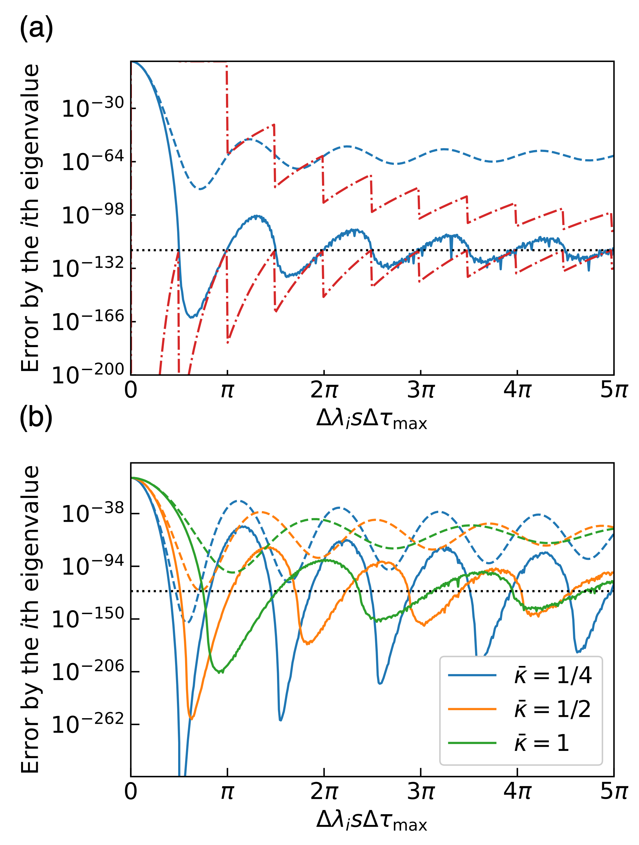
The error contributed by the th eigenvalue for linear scheduling is shown in Fig. 2(a). The logarithm of the error (blue solid line) exhibits damped oscillation, and ragged behavior is observed in the large- region. The ragged behavior of the error function is caused by the small number of steps . Increasing the number of steps was confirmed to result in a smoother curve. The error lies between the upper and lower bounds of the inequality. The arithmetic mean is larger than the geometric mean, but the behavior of the periodic function is similar. The error function and inequality are similar to those in Eq. (30) in the large- limit. According to the results shown in Fig. 2(a), we consider an optimal and in the linear scheduling. First, a smaller is preferable, because the larger denominator in Eq. (31) results in a smaller error. When , the arithmetic mean in Eq. (31) has the minimum value at . The calculated minimum point of the product is . In addition, the error contributed by the th eigenvalue increases as decreases for the region. Accordingly, we conclude that should be .
III.2.2 Exponential scheduling
Next, we investigate exponential scheduling Kosugi et al. 2022b; Kosugi et al. 2023, which is expressed as
| (32) |
for . Here, the parameter is introduced to adjust the speed of change of according to the increasing number of steps. A smaller value leads to a more rapid increase in . Note that, in the exponential scheduling based on Eq. (32), the imaginary-time step size in the final step differs from . In the th step, the maximum imaginary time is , where we define . The cumulative imaginary time for the exponential scheduling is calculated as
| (33) |
The analytical evaluation of the product is difficult; thus, we calculate the arithmetic mean of for exponential scheduling. The arithmetic mean , which is an approximation of the summation by integration, can be derived as
| (34) |
where we define and . The deviation of the phase of the cosine function is and the components of the amplitude are
| (35) |
The derivation of Eq. (34) and the expression of the sine integral and cosine integral are summarized in Appendix D.
The error contributed by the th eigenvalue for exponential scheduling is shown in Fig. 2(b). The ragged behavior of the error function (solid lines) caused by insufficient steps is observed. As in the linear-scheduling case, the error oscillates and asymptotically approaches Eq. (30), as indicated by the dashed black line, for all . In addition, the minimum and maximum peak positions depend on . The peak positions shift to larger values of as increases. We measure the minimum peak positions to be , , and for , 1/2, and 1, respectively. The error has the smallest value for .
This behavior can be explained understood as follows: First, a smaller leads to a faster change in the imaginary-time step . Thus, the error takes the smallest value of approximately -800 at the optimal because we mainly sample the optimal such that the error is small. However, the maximum error at the undesirable is enhanced compared with the larger . If is known in advance, can be adjusted to minimize the error. In contrast, a larger leads to a slower change; thus, the error is identical to that for linear scheduling. The advantage compared with the case where is small is that the error maxima are smaller. Accordingly, when is known, it is desirable to select a smaller in the exponential scheduling, whereas for an unknown , it is desirable to perform imaginary-time evolution with a larger or using linear scheduling. Next, we explain the reason for the shift in the position of the minimum peak. The imaginary time at the th step for exponential scheduling is smaller than . This reduction is more prominent for larger . In concrete terms, the final imaginary time with the minimum error is observed as , , and for , 1/2, and 1, respectively. We find that the final imaginary time is almost the same for all values, and the shift in the minimum peak position comes from keeping the final imaginary time constant. Thus, we should adopt such that the final imaginary time is approximately .
III.3 Error for all eigenvalues
Here, we consider the error contributed by all the eigenvalues. By changing the range of summation for in Eq. (21), we obtain
| (36) |
We introduce a distribution function as a function of eigenvalues to describe the probability weight of the initial state as . We assume that the distribution function is smooth along the eigenvalues and approximate the summation with the integral, which leads to
| (37) |
where represents the density of states (DOS) Grosso and Parravicini 2013. The distribution function satisfies . Here, and represent the minimum and maximum eigenvalues, respectively, and we define . Hereinafter, we denote and as and , respectively. This equation implies that the error depends on the distribution function and DOS originating from the initial state and Hamiltonian, respectively.
For a general DOS, deriving an explicit form of the errors in linear and exponential scheduling is difficult. Here, we consider the limit of large eigenvalues in the linear scheduling based on Eq. (30). By substituting (30) for (21), the error is written as
| (38) |
From this equation, we derive the number of steps required to achieve the error as
| (39) |
The corresponding total elapsed imaginary time for all steps for the linear scheduling is derived as
| (40) |
where and . For a larger , the total elapsed imaginary time is also obtained in exponential scheduling. A comparison with the exact ITE case in Eq.(6) reveals that the approximated PITE method requires additional ITE to achieve accuracy .
Equation (21) can be estimated in various ways. For example, we have
| (41) |

In the case of linear scheduling, the above inequality is satisfied by 1/3 of the total imaginary-time steps, as shown in Fig. 3. Thus, the needed steps are calculated as
| (42) |
The expression is identical to that in Eq. (39), except for the coefficients. When is set to an appropriate magnitude, exponential scheduling approaches linear scheduling, which enables a similar evaluation of the number of steps. Such estimates of computational cost have been discussed in the literature Meister and Benjamin 2022 but only for heuristic scheduling.
Let us estimate the computational cost for finding the smallest eigenvector of the Hamiltonian using PITE operations. From Eqs. (18) and (39), the scaling of computational time is expressed as
| (43) |
where represents the circuit depth of the quantum circuit for approximated PITE in Fig. 1(b). The depth can be regarded as the same scaling as the RTE operator because the approximated PITE circuit contains controlled-RTE operators. The depth also depends on the Hamiltonian and implementation of the RTE operators. Particularly, the Hamiltonian for an -electron system based on the first quantization requires the depth to be Kosugi et al. 2022a; Childs et al. 2021
| (44) |
where represents the grid spacing of the discretized space, and is the Trotter number dividing the RTE. The scaling of in the th-order Trotter–Suzuki decomposition is given by
| (45) |
where and Childs et al. 2021 with partial Hamiltonians such that . When choosing to be sufficiently large, the scaling of the Trotter number is expressed as . Now since the maximum in the linear and exponential scheduling is , the Trotter number scales as .
The estimated computational cost of the approximated PITE method scales as , where in Eq. (17) (see Eq. (43) in terms of ). This initial state dependence of the computational complexity is also observed in the Rodeo algorithm Choi et al. 2021; Meister and Benjamin 2022 and the ITE using quantum eigenvalue transform with unitary block encoding (QET-U) Chan et al. 2023. The computational cost of the QPE also depends on the initial state and scales as , where represents the statistical error Kitaev 1995; Abrams and Lloyd 1999. Therefore, even when the PITE method is used for the state preparation of QPE, the computational time of QPE does not change from that without PITE in terms of . However, although the computational advantage cannot be observed, the PITE method is useful for several reasons. For example, we cannot determine the true minimum eigenvalue using only QPE, because eigenvalues in the range of are folded in a finite interval. Even when we successfully specify the eigenvalues by unfolding them into the original interval , the minimum of the observed eigenvalues is not guaranteed to be the true minimum (the existence of smaller eigenvalues not observed yet cannot be ascertained.) Thus, systematic improvements to this problem may be difficult. One possibility to avoid the lack of acceleration is combining quantum amplitude amplification Brassard and Hoyer 1997; Brassard et al. 2000 with the PITE method, which results in a quadratic speedup Nishi et al. 2022. Constructing quantum circuits for preparing good initial states is also an important topic in ground-state preparation, and future research is required.
III.4 Validity of Taylor expansion for PITE
According to the discussion in Sec. III.2, we concluded that it is desirable to take ; however, one question arises here. In this case, we need to ascertain if is sufficiently small to execute the Taylor expansion for deriving the approximated PITE. can be significantly increased by increasing ; however, in this case, the coefficient of the quadratic term of the Taylor expansion in Eq. (7) becomes large. In this subsection, we discuss the computational cost for such that the Taylor expansion is valid, and the fact that the ground state can be obtained when is large.
First we estimate the computational cost for such that the Taylor expansion is valid. Let us consider the convergence condition when and are constant, regardless of the imaginary-time steps. The error contributed by the th eigenvalue in Eq. (16) per step should be smaller than 1 as , which is a necessary condition to achieve precision . In addition, we consider the shifting ground-state energy to be zero by applying a constant energy shift, where the approximation of the Taylor expansion is better for lower-energy states. In this constant energy shift, the necessary condition is expressed as
| (46) |
We must keep sufficiently small such that this condition holds for all eigenvalues . In this case, for example, if is chosen so that the left-hand side of Eq. (46) for is less than approximately , the upper bound of the error is expressed as
| (47) |
where we take . The upper bound indicates that a smaller or leads to increased error. This increase can be understood as follows: If a small is included in the Hamiltonian or if we progress through a gradual ITE process with a smaller , the decay of excited states is slow. As mentioned in Sec. III, the error is defined as the closeness of the approximately obtained state to the ground state; thus, the slow decay of the excited state increases the error. Of course, the approximation of the operator is better when is smaller. When we assume that is sufficiently large, the required number of steps such that error is satisfied is determined to be the same as that in Eq. (39). Additionally, the total imaginary time becomes
| (48) |
This equation implies that the imaginary-time evolution is times shorter than that in the case of linear and exponential scheduling. Therefore, additional imaginary-time steps may be required. In addition, if high-energy eigenstates are not included in the initial state, we can choose a larger , reducing the number of steps for obtaining the ground state.
According to the above discussion, we answer the previous question. In the original PITE, it is necessary to set sufficiently small so that the Taylor expansion holds for all eigenvalues . In contrast, in linear and exponential scheduling, it is possible to obtain the ground state without using the condition of such that the Taylor expansion is valid. By employing the constant energy shift given by Eq. (19), the error is minimized with respect to . The approximated PITE operator yields Eq. (20) that holds for any imaginary-time step size . Eq. (20) decays the other states than the ground state. The advantage of using linear and exponential scheduling is that it enables a constant energy shift such that the success probability is maximized. It is also expected to require fewer steps than constant scheduling. However, although the PITE method can be applied to Gibbs state calculations Kosugi et al. 2022a, whether we can directly adopt linear or exponential scheduling for Gibbs state calculations is unclear. This should be examined in the future.
IV Numerical simulations
To validate the analysis in Sec. III, we present numerical results for the Heisenberg chain. To examine the effect of the structure of the DOS, numerical results were also obtained for an electron under a double-well potential based on the first quantization form; these are presented in Appendix E.
IV.1 Setup
Here, we consider the spin Heisenberg model of a closed one-dimensional chain under a uniform magnetic field Choi et al. 2021. The Hamiltonian is expressed as
| (49) |
where is a three-dimensional vector of the Pauli matrices at site , represents the combination of nearest neighbors, represents the exchange coupling, and represents the strength of the uniform magnetic field. We used and , which correspond to the antiferromagnetic case. As an initial state, we used superposition with equal probability for all the eigenstates . The simulation was performed using qubits. The DOS of the Heisenberg chain is presented in Fig. 4, which was obtained via numerical diagonalization.

IV.2 Linear scheduling
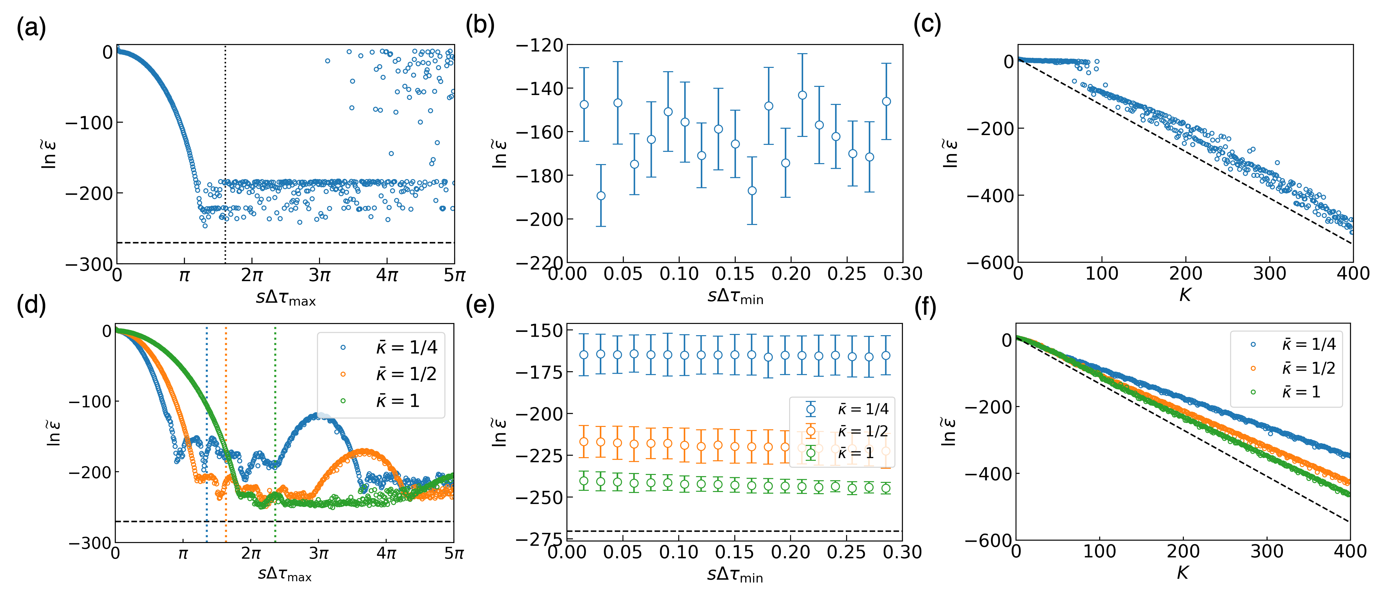
We show the error numerically calculated for linear scheduling in Figs. 5(a–c). In Fig. 5(a), as increases, the error decreases, and after the error reaches a minimum value at approximately , it becomes flat, with a slight increase. The optimal , which exhibits the minimum value in Fig. 5(a), is almost consistent with the optimal shown as a black dotted line, as discussed in Sec. III.2.1. The large error in the larger- region is prominent in the range . The reasons for the slight increase at a large are as follows: We calculated the error for each eigenvalue and found that the angles represented by Eq. (20) at which the largest errors occur are , where is an integer. Thus, even if varies for such eigenvalues, the angles are concentrated around for finite samplings, which causes a large error. In addition, the ragged behavior shown in Fig. 2(a) is exacerbated as increases, and we attribute this behavior to the same cause.
We show the error as a function of in Fig. 5(b). We also consider the effect of the deviation of from the minimum error positions of the th eigenvalue error. To consider this, we sampled the errors around the minimum error positions within the range of and plotted the mean and standard deviation for . The errors were randomly distributed according to ; thus, we could not observe the dependence of the error on , at least around the minimum error position. This implies that it is adequate to adopt a sufficiently small value for achieving a small error.
Finally, we examined the dependence of the error on the number of steps , as shown in Fig. 5(c). For the optimal , the error agreed well with the theoretically estimated value based on Eq. (30); i.e., the error decreased exponentially with an increase in the number of steps. If we use a suboptimal imaginary-time step size, the deviation from the theoretical value should be increased.
IV.3 Exponential scheduling
Figure 5(d) shows the error in exponential scheduling according to . Similar to the linear-scheduling case, the error for exponential scheduling decreased as increased, and the minimum values are shown at the minimum peak positions, as plotted with dotted lines in Fig. 5(b) for all . However, the logarithmic errors depend on . In addition, the errors exhibit upper convex peaks after the minimum peak positions. A smaller indicates a larger maximum, which is caused by the rapid change in leading to biased sampling around a specific angle, as discussed in Sec. III.2.2. Surprisingly, the error can be maintained at a small value in the larger- region compared with linear scheduling. This is because the nonlinear change in avoids biased sampling around a specific angle even when we have . Thus, we can suppress the error in the larger-suboptimal region for exponential scheduling.
We plot the means and standard deviations of the errors around the minimum peak positions in Fig. 5(e). Here, we do not observe a dependence of the error on , similar to the linear-scheduling case. The errors decrease when as increases.
The error is plotted with respect to the number of steps in Fig. 5(f). We observe an exponential decay of the error as the number of steps increases. The deviations from the theoretical values are smaller when is larger. In addition, the degree of scattering within the line is smaller than that in the case of linear scheduling. According to the results of the numerical simulations, exponential scheduling with a large is preferable for suppressing the error and reducing the number of PITE steps.
IV.4 Discussion of optimal scheduling
Based on the analytical and numerical results for linear and exponential scheduling, we discuss optimal scheduling for the approximated PITE method. In Sec. III.2, if the eigenvalues are unknown, we concluded that it is desirable to choose a larger in exponential scheduling or to use linear scheduling. This conclusion is based on the requirement that the error contributed by an undesirable eigenvalue must be small (see the maximum values in Fig. 2). Linear scheduling is the most desirable method due to its sampling of all eigenvalues equally. By contrast, the numerical simulations presented in Secs. IV.2 and IV.3 reveal that linear scheduling produces a larger error for large (See Fig. 5(a)). This large error is caused by the fact that for integers , the angle of the cosine function is expressed as and concentrates around , even when the imaginary-time step size is changed linearly. Nonlinear changes are necessary to avoid concentration around a specific value. In conclusion, a scheduling that changes linearly for the most part but includes nonlinear changes is desirable for imaginary-time scheduling in the approximated PITE.
V Conclusions
We investigated the computational cost of a PITE method that implements a nonunitary ITE operator on a quantum computer with a single ancilla qubit. Particularly, we considered an approximated PITE circuit within a first-order imaginary-time step consisting of forward and backward controlled-RTE operators. We defined and evaluated an error describing the closeness between the wave functions acted on by the exact and approximate ITE operators. First, we analytically evaluated the contribution of one eigenvalue of a given Hamiltonian to the error for both linear and exponential scheduling. In addition, we estimated the optimal imaginary-time step size and discussed the scheduling speed. Next, we discussed the error contributed by all the eigenvalues, from which the number of steps needed to achieve precision is estimated as , where is the probability weight of the ground state in the initial state. When we implement each PITE step at depth , the total computational cost, including the measurements, is . To validate this findings, we numerically simulated the error for a one-dimensional Heisenberg chain. From the analytical evaluation, we found that linear scheduling works well in the case of unknown eigenvalues of the Hamiltonian, and returns smaller errors on average for a wide range of eigenstates. However, the numerical simulation revealed that the linearity of the scheduling causes problems for some specific energy regions of the eigenstates. To avoid this problem, including nonlinearity, such as by exponential scheduling, is preferable for reducing the computational cost, even with a suboptimal imaginary-time step size. The findings of this research can contribute significantly to the ground-state calculation of quantum many-body problems using quantum computers.
Acknowledgments
This work was supported by MEXT under ”Program for Promoting Researches on the Supercomputer Fugaku” (JPMXP1020200205) and by JSPS KAKENHI under Grant-in-Aid for Scientific Research (A) No. 21H04553.
Appendix A Increase and decrease in success probability
A monotonic increase in the success probability was proven for a two-level system Kosugi et al. 2022a. Here, we extend the proof to a more general case. The success probability at the th step is expressed as
| (50) |
The difference in the success probability is expressed as
| (51) |
Its sign at each step is determined only by the numerator on the right-hand side. The numerator of Eq. (51) is rewritten with Eq. (12) as
| (52) |
Here, we transform as follows:
| (53) |
The second term in Eq. (53) can be proven to be positive:
| (54) |
If the inequality is satisfied for any , the first term in Eq. (53) is positive. Additionally, if does not depend on , the first term vanishes. In this case, we have .
Appendix B Effect of constant energy shift on the total success probability
We examine the effect of the constant energy shift given by Eq. (19) on the total success probability . Consider a parameter that changes the constant energy shift, the value of which is expressed as
| (55) |
When we set and , the total success probability given by Eq. (18) changes to
| (56) |
and
| (57) |
respectively.

We plotted the total success probability according to the parameter in the constant energy shift in Fig. 6. As a computational target, we used the Heisenberg model of a closed one-dimensional chain with spins, as in Sec. IV. Exponential scaling with , and was adopted, which is the optimal scheduling as discussed in Sec. IV. We set and the initial state as a uniformly weighted distribution. When , the total success probabilities are and for and , respectively. The values of for in Fig. 6 are consistent with Eq. (56). Conversely, the total success probability increases and takes the maximum value at . This maximum value is consistent with Eq. (57).
Appendix C Derivation of inequality and arithmetic mean in linear scheduling
First, we derive the inequality given by Eq. (28). For linear scheduling based on Eq.(26), the logarithm of the error in Eq.(23) is rewritten as
| (58) |
where we define and . We substitute for , which leads to
| (59) |
Here, the following relationship holds:
| (60) |
Additionally, we can derive for an integer . Thus, the integral is bounded as
| (61) |
For the large eigenvalues , the integral in Eq. (61) becomes
| (62) |
Next, we derive the arithmetic mean , which is an approximation of the summation by integration, for the linear scheduling based on Eq. (26). By substituting into Eq. (26), the arithmetic mean in Eq. (25) is rewritten as
| (63) |
By applying , we have
| (64) |
where the final equation corresponds to Eq. (31).
Appendix D Derivation of arithmetic mean for exponential scheduling
Here, we present the derivation of the arithmetic mean in Eq. (25), which is an approximation of the summation by integration, for exponential scheduling based on Eq. (32), as expressed in Eq. (34). The arithmetic mean for exponential scheduling is calculated as
| (65) |
where we define and . Applying leads to
| (66) |
Eq. (66) is rewritten as
| (67) |
where . Additionally, we use the sine integral
| (68) |
and the related function of the cosine integral
| (69) |
where the cosine integral is rewritten as
| (70) |
Here, is Euler’s constant. The trigonometric function in Eq. (67) is expressed using single cosine function:
| (71) |
where and
| (72) |

The limits of the sine and cosine integrals are and , respectively. For the large eigenvalues , the arithmetic mean becomes , because and . Additionally, in the small- limit , Eq. (67) changes as follows: This indicates that quickly reaches , and then the state evolves imaginary time by a constant time step . In contrast, when is larger, the arithmetic mean becomes because does not change from in such a limit.
To further examine the dependence of Eq. (71) on , we plot the coefficients and the deviation of the phase in Fig. 7. The amplitude of the cosine function decreases with the oscillation as increases. Thus, the arithmetic mean in the exponential scheduling approaches 1/2, as shown in Fig. 2. The deviation of the phase that corresponds to the peak position of the arithmetic mean increases as increases. This increase implies that the frequency of the maximum and minimum in the arithmetic mean is higher than that in the small- region. In addition, this increasing frequency is prominent for larger .
Appendix E Numerical simulations for other Hamiltonians
E.1 Asymmetric double-well potential
E.1.1 Setup
To determine the influence of the DOS, the numerical results of the error calculations for different Hamiltonians are examined in this section. The approximated PITE method was proposed as a first quantum eigensolver to solve problems based on the first quantization Hamiltonian Kosugi et al. 2022a. Historically, quantum algorithms for the RTE of the first quantization Hamiltonian were proposed by Zalka Zalka 1998 and Wiesner Wiesner 1996. The wave functions of each grid in a discretized space can be encoded on an exponential basis on a quantum computer, and the real space and momentum space can be transformed by a quantum Fourier transform Nielsen et al. 2000; Somma 2015; Ollitrault et al. 2020. In recent years, various quantum circuit implementations for the RTE operator of the first quantization Hamiltonian have been proposed Kassal et al. 2008; Kivlichan et al. 2017; Babbush et al. 2018; Babbush et al. 2019; Su et al. 2021.
In this section, we present the results for the problem of a single electron in a one-dimensional asymmetric double-well potential as a numerical example from the literature Kosugi et al. 2022a. A double-well potential defined as
| (73) |
is used for the simulations. We set the length of the simulation cell as , the distance between minima as , the height of the higher minimum measured from the smaller minimum as , and the strength of the barrier between the minima as .

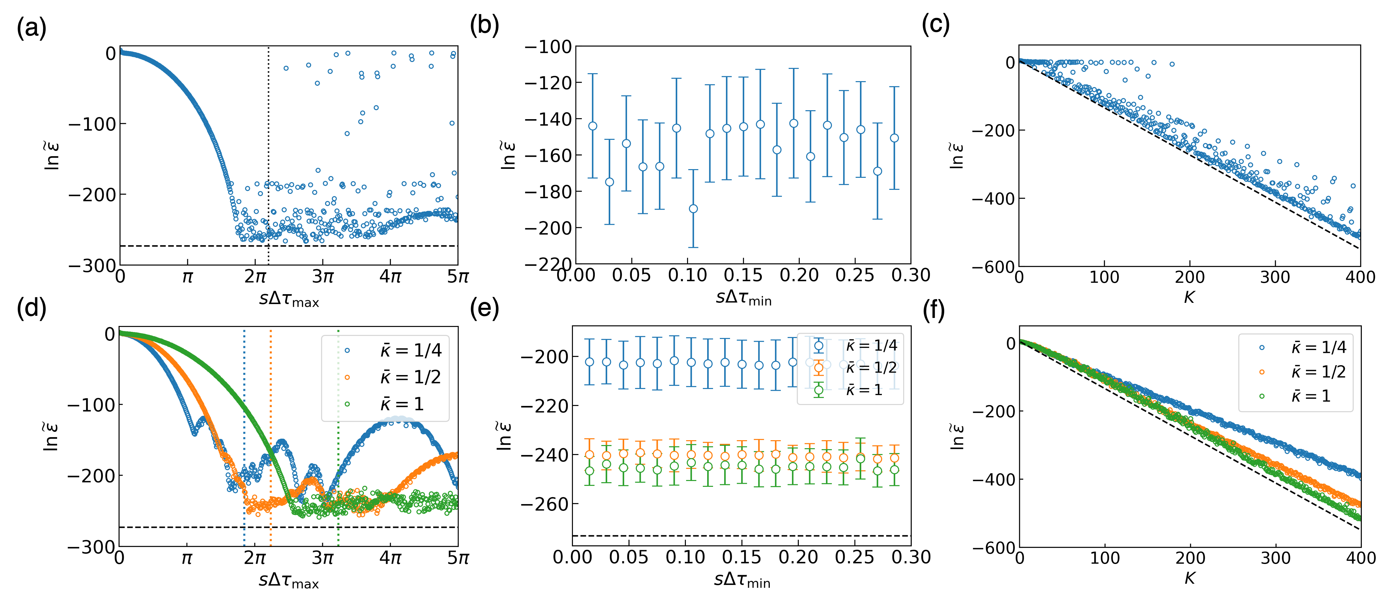
The numerical diagonalization results for this Hamiltonian with six qubits are shown in Fig. 8. We used an electron mass of and a Planck constant of in the simulation. Equal probability weights were adopted as the initial state. In contrast to the Heisenberg chain, the DOS of the double-well potential was almost independent of the eigenvalue, as in the case of the harmonic potential. Note that the sparseness for the higher eigenvalues is caused by the finite cell size.
E.1.2 Linear scheduling
The logarithmic error for an electron in the asymmetric double-well potential is shown in Figs. 8(a–c) for linear scheduling. This basic behavior is similar to the results for the one-dimensional Heisenberg chain in Sec. IV. From Fig. 8(a), there is no flat behavior in the region larger than the minimum error position, and a peak-like behavior is observed. This is attributed to sampling bias, which results in a larger error, becoming smaller than the results of the Heisenberg chain because the number of qubits or eigenvalues is small. In Fig. 8(b), we similarly observe that the error is independent of . In Fig. 8(c), the dependence of the error on the number of steps is found to be consistent with the expression for the large eigenvalue limit in Eq. (30).
E.1.3 Exponential scheduling
The dependence of the error on is illustrated in Fig. 8(d). The error decreases as increases, and an upper convex peak is observed after the minimum error is reached. The size and position of this peak depend on . The error is plotted as a function of in Fig. 8(e), and no dependence of error on is observed for all . The error decays exponentially as the number of steps increases, and its behavior approaches Eq. (30) for a larger . These behaviors are consistent with the results of the Heisenberg chain calculations presented in Sec. IV.
References
- Cirac and Zoller (1995) J. I. Cirac and P. Zoller, Quantum computations with cold trapped ions, Phys. Rev. Lett. 74, 4091 (1995).
- Nakamura et al. (1999) Y. Nakamura, Y. A. Pashkin, and J. Tsai, Coherent control of macroscopic quantum states in a single-cooper-pair box, nature 398, 786 (1999).
- Bruzewicz et al. (2019) C. D. Bruzewicz, J. Chiaverini, R. McConnell, and J. M. Sage, Trapped-ion quantum computing: Progress and challenges, Applied Physics Reviews 6, 021314 (2019).
- Krantz et al. (2019) P. Krantz, M. Kjaergaard, F. Yan, T. P. Orlando, S. Gustavsson, and W. D. Oliver, A quantum engineer’s guide to superconducting qubits, Applied physics reviews 6, 021318 (2019).
- Arute et al. (2019) F. Arute, K. Arya, R. Babbush, D. Bacon, J. C. Bardin, R. Barends, R. Biswas, S. Boixo, F. G. Brandao, D. A. Buell, et al., Quantum supremacy using a programmable superconducting processor, Nature 574, 505 (2019).
- Feynman (1982) R. P. Feynman, Simulating physics with computers, International Journal of Theoretical Physics 21 (1982).
- Grover (1996) L. K. Grover, A fast quantum mechanical algorithm for database search, in Proceedings of the twenty-eighth annual ACM symposium on Theory of computing (1996) pp. 212–219.
- Shor (1999) P. W. Shor, Polynomial-time algorithms for prime factorization and discrete logarithms on a quantum computer, SIAM Review 41, 303 (1999), https://doi.org/10.1137/S0036144598347011 .
- Lloyd (1996) S. Lloyd, Universal quantum simulators, Science 273, 1073 (1996), https://www.science.org/doi/pdf/10.1126/science.273.5278.1073 .
- Berry et al. (2015) D. W. Berry, A. M. Childs, R. Cleve, R. Kothari, and R. D. Somma, Simulating hamiltonian dynamics with a truncated taylor series, Phys. Rev. Lett. 114, 090502 (2015).
- Low and Chuang (2017) G. H. Low and I. L. Chuang, Optimal hamiltonian simulation by quantum signal processing, Phys. Rev. Lett. 118, 010501 (2017).
- Gilyén et al. (2019) A. Gilyén, Y. Su, G. H. Low, and N. Wiebe, Quantum singular value transformation and beyond: Exponential improvements for quantum matrix arithmetics, in Proceedings of the 51st Annual ACM SIGACT Symposium on Theory of Computing, STOC 2019 (Association for Computing Machinery, New York, NY, USA, 2019) p. 193–204.
- Martyn et al. (2021) J. M. Martyn, Z. M. Rossi, A. K. Tan, and I. L. Chuang, Grand unification of quantum algorithms, PRX Quantum 2, 040203 (2021).
- Farhi et al. (2000) E. Farhi, J. Goldstone, S. Gutmann, and M. Sipser, Quantum computation by adiabatic evolution (2000).
- Aspuru-Guzik et al. (2005) A. Aspuru-Guzik, A. D. Dutoi, P. J. Love, and M. Head-Gordon, Simulated quantum computation of molecular energies, Science 309, 1704 (2005), https://www.science.org/doi/pdf/10.1126/science.1113479 .
- Poulin and Wocjan (2009) D. Poulin and P. Wocjan, Preparing ground states of quantum many-body systems on a quantum computer, Phys. Rev. Lett. 102, 130503 (2009).
- Ge et al. (2019) Y. Ge, J. Tura, and J. I. Cirac, Faster ground state preparation and high-precision ground energy estimation with fewer qubits, Journal of Mathematical Physics 60, 022202 (2019).
- Lin and Tong (2020) L. Lin and Y. Tong, Near-optimal ground state preparation, Quantum 4, 372 (2020).
- Cao et al. (2019) Y. Cao, J. Romero, J. P. Olson, M. Degroote, P. D. Johnson, M. Kieferová, I. D. Kivlichan, T. Menke, B. Peropadre, N. P. D. Sawaya, S. Sim, L. Veis, and A. Aspuru-Guzik, Quantum chemistry in the age of quantum computing, Chemical Reviews 119, 10856 (2019), pMID: 31469277, https://doi.org/10.1021/acs.chemrev.8b00803 .
- McArdle et al. (2020) S. McArdle, S. Endo, A. Aspuru-Guzik, S. C. Benjamin, and X. Yuan, Quantum computational chemistry, Rev. Mod. Phys. 92, 015003 (2020).
- Bauer et al. (2020) B. Bauer, S. Bravyi, M. Motta, and G. K.-L. Chan, Quantum algorithms for quantum chemistry and quantum materials science, Chemical Reviews 120, 12685 (2020), pMID: 33090772, https://doi.org/10.1021/acs.chemrev.9b00829 .
- Peruzzo et al. (2014) A. Peruzzo, J. McClean, P. Shadbolt, M.-H. Yung, X.-Q. Zhou, P. J. Love, A. Aspuru-Guzik, and J. L. O’brien, A variational eigenvalue solver on a photonic quantum processor, Nature communications 5, 1 (2014).
- Farhi et al. (2014) E. Farhi, J. Goldstone, and S. Gutmann, A quantum approximate optimization algorithm, arXiv preprint arXiv:1411.4028 https://doi.org/10.48550/arXiv.1411.4028 (2014).
- Yuan et al. (2019) X. Yuan, S. Endo, Q. Zhao, Y. Li, and S. C. Benjamin, Theory of variational quantum simulation, Quantum 3, 191 (2019).
- McArdle et al. (2019) S. McArdle, T. Jones, S. Endo, Y. Li, S. C. Benjamin, and X. Yuan, Variational ansatz-based quantum simulation of imaginary time evolution, npj Quantum Information 5, 75 (2019).
- Motta et al. (2020) M. Motta, C. Sun, A. T. Tan, M. J. O’Rourke, E. Ye, A. J. Minnich, F. G. Brandao, and G. K. Chan, Determining eigenstates and thermal states on a quantum computer using quantum imaginary time evolution, Nature Physics 16, 205 (2020).
- Seki and Yunoki (2021) K. Seki and S. Yunoki, Quantum power method by a superposition of time-evolved states, PRX Quantum 2, 010333 (2021).
- Shor (1995) P. W. Shor, Scheme for reducing decoherence in quantum computer memory, Phys. Rev. A 52, R2493 (1995).
- Knill et al. (1998) E. Knill, R. Laflamme, and W. H. Zurek, Resilient quantum computation, Science 279, 342 (1998), https://www.science.org/doi/pdf/10.1126/science.279.5349.342 .
- Krinner et al. (2022) S. Krinner, N. Lacroix, A. Remm, A. Di Paolo, E. Genois, C. Leroux, C. Hellings, S. Lazar, F. Swiadek, J. Herrmann, et al., Realizing repeated quantum error correction in a distance-three surface code, Nature 605, 669 (2022).
- Acharya et al. (2023) R. Acharya, I. Aleiner, R. Allen, T. I. Andersen, M. Ansmann, F. Arute, K. Arya, A. Asfaw, J. Atalaya, R. Babbush, et al., Suppressing quantum errors by scaling a surface code logical qubit, Nature 614, 676 (2023).
- Temme et al. (2017) K. Temme, S. Bravyi, and J. M. Gambetta, Error mitigation for short-depth quantum circuits, Phys. Rev. Lett. 119, 180509 (2017).
- Endo et al. (2018) S. Endo, S. C. Benjamin, and Y. Li, Practical quantum error mitigation for near-future applications, Phys. Rev. X 8, 031027 (2018).
- Koczor (2021) B. Koczor, Exponential error suppression for near-term quantum devices, Phys. Rev. X 11, 031057 (2021).
- Huggins et al. (2021) W. J. Huggins, S. McArdle, T. E. O’Brien, J. Lee, N. C. Rubin, S. Boixo, K. B. Whaley, R. Babbush, and J. R. McClean, Virtual distillation for quantum error mitigation, Phys. Rev. X 11, 041036 (2021).
- Endo et al. (2021) S. Endo, Z. Cai, S. C. Benjamin, and X. Yuan, Hybrid quantum-classical algorithms and quantum error mitigation, Journal of the Physical Society of Japan 90, 032001 (2021), https://doi.org/10.7566/JPSJ.90.032001 .
- Hama and Nishi (2022) Y. Hama and H. Nishi, Quantum error mitigation via quantum-noise-effect circuit groups (2022).
- Cai et al. (2022) Z. Cai, R. Babbush, S. C. Benjamin, S. Endo, W. J. Huggins, Y. Li, J. R. McClean, and T. E. O’Brien, Quantum error mitigation (2022).
- Tong (2022) Y. Tong, Designing algorithms for estimating ground state properties on early fault-tolerant quantum computers, Quantum Views 6, 65 (2022).
- Zhang et al. (2022) R. Zhang, G. Wang, and P. Johnson, Computing Ground State Properties with Early Fault-Tolerant Quantum Computers, Quantum 6, 761 (2022).
- Campbell (2021) E. T. Campbell, Early fault-tolerant simulations of the hubbard model, Quantum Science and Technology 7, 015007 (2021).
- Lin and Tong (2022) L. Lin and Y. Tong, Heisenberg-limited ground-state energy estimation for early fault-tolerant quantum computers, PRX Quantum 3, 010318 (2022).
- Wang et al. (2022) G. Wang, S. Sim, and P. D. Johnson, State Preparation Boosters for Early Fault-Tolerant Quantum Computation, Quantum 6, 829 (2022).
- Wan et al. (2022) K. Wan, M. Berta, and E. T. Campbell, Randomized quantum algorithm for statistical phase estimation, Phys. Rev. Lett. 129, 030503 (2022).
- Dong et al. (2022) Y. Dong, L. Lin, and Y. Tong, Ground-state preparation and energy estimation on early fault-tolerant quantum computers via quantum eigenvalue transformation of unitary matrices, PRX Quantum 3, 040305 (2022).
- Kitaev (1995) A. Y. Kitaev, Quantum measurements and the abelian stabilizer problem (1995).
- Abrams and Lloyd (1999) D. S. Abrams and S. Lloyd, Quantum algorithm providing exponential speed increase for finding eigenvalues and eigenvectors, Phys. Rev. Lett. 83, 5162 (1999).
- Choi et al. (2021) K. Choi, D. Lee, J. Bonitati, Z. Qian, and J. Watkins, Rodeo algorithm for quantum computing, Phys. Rev. Lett. 127, 040505 (2021).
- Silva et al. (2021) T. d. L. Silva, M. M. Taddei, S. Carrazza, and L. Aolita, Fragmented imaginary-time evolution for early-stage quantum signal processors (2021).
- Kosugi et al. (2022a) T. Kosugi, Y. Nishiya, H. Nishi, and Y.-i. Matsushita, Imaginary-time evolution using forward and backward real-time evolution with a single ancilla: First-quantized eigensolver algorithm for quantum chemistry, Phys. Rev. Research 4, 033121 (2022a).
- Meister and Benjamin (2022) R. Meister and S. C. Benjamin, Resource-frugal hamiltonian eigenstate preparation via repeated quantum phase estimation measurements (2022).
- Stetcu et al. (2022) I. Stetcu, A. Baroni, and J. Carlson, Projection algorithm for state preparation on quantum computers (2022).
- Xie et al. (2022a) H.-N. Xie, S.-J. Wei, F. Yang, Z.-A. Wang, C.-T. Chen, H. Fan, and G.-L. Long, A probabilistic imaginary time evolution algorithm based on non-unitary quantum circuit (2022a).
- Xie et al. (2022b) Q.-X. Xie, Y. Song, and Y. Zhao, Power of the sine hamiltonian operator for estimating the eigenstate energies on quantum computers, Journal of Chemical Theory and Computation 18, 7586 (2022b), pMID: 36449783, https://doi.org/10.1021/acs.jctc.2c00759 .
- Chan et al. (2023) H. H. S. Chan, D. Muñoz-Ramo, and N. Fitzpatrick, Simulating non-unitary dynamics using quantum signal processing with unitary block encoding (2023).
- Kosugi et al. (2022b) T. Kosugi, H. Nishi, and Y. Matsushita, Exhaustive search for optimal molecular geometries using imaginary-time evolution on a quantum computer (2022b).
- Kosugi et al. (2023) T. Kosugi, H. Nishi, and Y. ichiro Matsushita, First-quantized eigensolver for ground and excited states of electrons under a uniform magnetic field, Japanese Journal of Applied Physics 62, 062004 (2023).
- Kitaev et al. (2002) A. Y. Kitaev, A. Shen, and M. N. Vyalyi, Classical and quantum computation, 47 (American Mathematical Soc., 2002).
- Kempe et al. (2005) J. Kempe, A. Kitaev, and O. Regev, The complexity of the local hamiltonian problem, in FSTTCS 2004: Foundations of Software Technology and Theoretical Computer Science, edited by K. Lodaya and M. Mahajan (Springer Berlin Heidelberg, Berlin, Heidelberg, 2005) pp. 372–383.
- Oliveira and Terhal (2008) R. Oliveira and B. M. Terhal, The complexity of quantum spin systems on a two-dimensional square lattice (2008), arXiv:quant-ph/0504050 [quant-ph] .
- Grosso and Parravicini (2013) G. Grosso and G. P. Parravicini, Solid state physics, 2nd ed. (Academic press, 2013).
- Childs et al. (2021) A. M. Childs, Y. Su, M. C. Tran, N. Wiebe, and S. Zhu, Theory of trotter error with commutator scaling, Phys. Rev. X 11, 011020 (2021).
- Brassard and Hoyer (1997) G. Brassard and P. Hoyer, An exact quantum polynomial-time algorithm for simon’s problem, in Proceedings of the Fifth Israeli Symposium on Theory of Computing and Systems (1997) pp. 12–23.
- Brassard et al. (2000) G. Brassard, P. Hoyer, M. Mosca, and A. Tapp, Quantum Amplitude Amplification and Estimation, arXiv e-prints , quant-ph/0005055 (2000), arXiv:quant-ph/0005055 [quant-ph] .
- Nishi et al. (2022) H. Nishi, T. Kosugi, Y. Nishiya, and Y.-i. Matsushita, Acceleration of probabilistic imaginary-time evolution method combined with quantum amplitude amplification (2022).
- Zalka (1998) C. Zalka, Simulating quantum systems on a quantum computer, Proceedings of the Royal Society of London. Series A: Mathematical, Physical and Engineering Sciences 454, 313 (1998).
- Wiesner (1996) S. Wiesner, Simulations of many-body quantum systems by a quantum computer (1996).
- Nielsen et al. (2000) M. A. Nielsen, I. L. Chuang, I. L. Chuang, et al., Quantum Computation and Quantum Information (Cambridge University Press, 2000).
- Somma (2015) R. D. Somma, Quantum simulations of one dimensional quantum systems (2015).
- Ollitrault et al. (2020) P. J. Ollitrault, G. Mazzola, and I. Tavernelli, Nonadiabatic molecular quantum dynamics with quantum computers, Phys. Rev. Lett. 125, 260511 (2020).
- Kassal et al. (2008) I. Kassal, S. P. Jordan, P. J. Love, M. Mohseni, and A. Aspuru-Guzik, Polynomial-time quantum algorithm for the simulation of chemical dynamics, Proceedings of the National Academy of Sciences 105, 18681 (2008), https://www.pnas.org/doi/pdf/10.1073/pnas.0808245105 .
- Kivlichan et al. (2017) I. D. Kivlichan, N. Wiebe, R. Babbush, and A. Aspuru-Guzik, Bounding the costs of quantum simulation of many-body physics in real space, Journal of Physics A: Mathematical and Theoretical 50, 305301 (2017).
- Babbush et al. (2018) R. Babbush, N. Wiebe, J. McClean, J. McClain, H. Neven, and G. K.-L. Chan, Low-depth quantum simulation of materials, Phys. Rev. X 8, 011044 (2018).
- Babbush et al. (2019) R. Babbush, D. W. Berry, J. R. McClean, and H. Neven, Quantum simulation of chemistry with sublinear scaling in basis size, npj Quantum Information 5, 92 (2019).
- Su et al. (2021) Y. Su, D. W. Berry, N. Wiebe, N. Rubin, and R. Babbush, Fault-tolerant quantum simulations of chemistry in first quantization, PRX Quantum 2, 040332 (2021).