Quantum Alternating Operator Ansatz (QAOA) beyond
low depth with gradually changing unitaries
Abstract
The Quantum Approximate Optimization Algorithm and its generalization to Quantum Alternating Operator Ansätze (QAOA) is a promising approach for applying quantum computers to challenging problems such as combinatorial optimization and computational chemistry. In this paper, we study the underlying mechanisms governing the behavior of QAOA circuits beyond shallow depth in the practically relevant setting of gradually varying unitaries. We use the discrete adiabatic theorem, which complements and generalizes the insights obtained from the continuous-time adiabatic theorem primarily considered in prior work. Our analysis explains some general properties that are conspicuously depicted in the recently introduced QAOA performance diagrams. For parameter sequences derived from continuous schedules (e.g. linear ramps), these diagrams capture the algorithm’s performance over different parameter sizes and circuit depths. Surprisingly, they have been observed to be qualitatively similar across different performance metrics and application domains. Our analysis explains this behavior as well as entails some unexpected results, such as connections between the eigenstates of the cost and mixer QAOA Hamiltonians changing based on parameter size and the possibility of reducing circuit depth without sacrificing performance.
1 Introduction
Quantum computing presents numerous promising approaches to challenging computational problems across a wide variety of applications. Among these approaches are the Quantum Approximate Optimization Algorithm Farhi et al. 2014 and Quantum Alternating Operator Ansatz (QAOA) Hadfield et al. 2019, developed to solve classical combinatorial optimization problems, and later extended to more general tasks such as state preparation Ho and Hsieh 2019; Kremenetski et al. 2021a. In its simplest realization, given a cost Hamiltonian to optimize, the protocol starts with the ground state of a mixer Hamiltonian and then proceeds by alternately evolving the state under the two Hamiltonians times each. While there are results on QAOA behavior for small Farhi and Harrow 2016; Wang et al. 2018; Wurtz and Love 2021; Vikstål et al. 2020; Díez-Valle et al. 2022; Akshay et al. 2022; Streif and Leib 2019 and in some cases Farhi et al. 2014; Jiang et al. 2017; Kim et al. 2021; Koßmann et al. 2022, there remains the challenge of understanding the behavior of QAOA more broadly. Generally, QAOA is characterized by parameters that represent how long the Hamiltonians are simulated at each step in the protocol, and therefore parameter setting is expected to become challenging as grows Zhou et al. 2020; Leng et al. 2022; Wurtz and Lykov 2021; Brady et al. 2021; Koßmann et al. 2022.
To better understand the behavior of QAOA, we introduce an approach to analyzing deep circuits with gradually varying unitaries. This extends beyond the small-parameter regime of QAOA considered as Trotterized annealing in prior work Farhi et al. 2014; Kocia et al. 2022; Sack and Serbyn 2021a; Pelofske et al. 2023. Through our analysis, we show such deep circuits exhibit surprising phenomena. One is the ground state of the mixer Hamiltonian directly connecting to a highly excited state of the cost Hamiltonian, resulting in poor QAOA performance even in an adiabatic limit. Another is shallower circuits outperforming deeper ones at large parameters due to inherently non-adiabatic effects (performing comparably to deeper circuits at smaller parameters). We also show how these phenomena, along with small-parameter approximations, explain a general qualitative feature Kremenetski et al. 2021a in performance for deep QAOA circuits with slowly varying parameters.
Specifically, we apply the discrete adiabatic theorem Dranov et al. 1998. This theorem is a generalization of the continuous adiabatic theorem, where a state evolving in time tracks an eigenstate across a product of gradually varying unitaries rather than the eigenstate of a slowly changing Hamiltonian. Since unitary eigenvalues can wrap around the complex unit circle and produce avoided crossings, when QAOA parameters are large, this wrap-around leads to the mixer ground state becoming connected to a high-lying cost excited state. This change in connectivity is described by the mathematical theory of holonomy Cheon et al. 2009 that generalizes the well-known phenomenon of Berry phase Berry 1984; Wilczek and Zee 1984. Consequently, the state resulting from QAOA has high support on the high-lying excited state in the discrete adiabatic limit (arbitrarily large ). Outside of this limit, we characterize how well the state tracks the changing eigenstate through small gaps using a discretized Landau-Zener formula.

This new analysis explains the performance features of QAOA seen in a recent study Kremenetski et al. 2021a that applied QAOA with parameters derived from a linear ramp to electronic structure problems. Qualitatively similar behavior in performance was observed for intermediate and in the limit for large angles across a wide variety of problems, a generality that persisted with nonlinear, smooth schedules. The general nature of this behavior is sketched in Fig. 1. The labels in Fig. 1 indicate regions with qualitatively different performance, though the regions are not entirely disjoint and the boundaries between them are not sharp. To the left and bottom of the diagram (labeled Initial State), the performance is low and close to that of the starting state; while in the lower-right region (High), the performance is high and approaches continuous adiabatic behavior. The upper-right region (Low) has very poor performance. At the bottom, QAOA in the Annealing region closely approximates continuous annealing. Toward the upper left, the Ridge region has relatively high performance. At large values of , there is a sudden drop in performance when the angle size exceeds a threshold value: an abrupt change between High and Low regions. In this paper, we argue that this performance drop is due to a change in connectivity of eigenstates associated with QAOA operators, which causes the QAOA state vector to end in an excited state of the cost Hamiltonian.
The paper is structured as follows. We introduce QAOA in Section 2. Section 3 introduces the discrete adiabatic theorem. Section 4 studies the connections between eigenstates of the product pairs of unitaries that make up a QAOA protocol. Section 5 introduces and explains the qualitative generality of QAOA performance diagrams. Section 6 gives examples with more complex performance diagram behavior, and Section 7 illustrates how our results apply to schedules with gradually changing angles beyond those easily captured by performance diagrams and how these diagrams scale with problem size. Additional technical derivations are provided as appendices.
2 QAOA with gradually changing parameters
For QAOA, a given optimization problem on variables is encoded as a cost Hamiltonian on qubits. Level- QAOA uses and a suitably chosen mixer Hamiltonian to apply parameterized unitary operators
| (1) |
for , with parameters and , also referred to as “angles”. We refer to the operators and as the mixer and cost unitaries, respectively. We consider the general setting for QAOA, where the mixer and the cost Hamiltonians do not commute but are otherwise arbitrary Hadfield et al. 2019, which includes a wide range of problems from combinatorial optimization as well as quantum chemistry Kremenetski et al. 2021a.
QAOA starts with an easily prepared initial state , which is typically the ground state of . For example, for the originally proposed transverse-field mixer (also known as the -mixer) , , an equally weighted superposition over the computational basis. QAOA produces the output state
| (2) |
Ideally, this QAOA output state has high overlap with the ground state of . For combinatorial optimization, it suffices to have non-negligible support on the ground state in order to solve the problem with repeated state preparation and measurement, though for challenging problems we often must settle for an approximate solution i.e., obtaining sufficient support on a low-lying eigenstate. On the other hand, chemistry applications such as electronic structure problems often require a much higher overlap with the true ground state Kremenetski et al. 2021a.
A common measure of the effectiveness of QAOA is the expected cost (or energy) of the output state . Typically, it may be efficiently estimated via repeated preparations and measurements. In some cases this quantity is used as a proxy for the true overlap with the ground state, which may be as difficult to compute as the underlying problem itself. On the other hand, for small or moderately sized benchmarking problems we may often compute the ground state overlap directly Kremenetski et al. 2021a; Willsch et al. 2020. We provide empirical evidence that both metrics produce similar phenomena, though we primarily use ground state overlap as the QAOA performance metric.
We consider QAOA parameter schedules with gradually changing parameters, i.e., schedules for which are small (relative to the inverse of the norms of and ). Specifically, we consider a continuous schedule to be one generated through samples from continuous functions on , so that , where
| (3) |
for , and . For simplicity, we focus on linear ramps
| (4) |
where is a constant. Section 7 discusses more general schedules.
For the linear schedule of Eqs. (3) and (4), the QAOA unitary of Eq. (1) becomes
| (5) |
for fixed . Similar linear schedules are frequently considered for QAOA in optimization settings Hogg 2000; Crooks 2018; Bigan Mbeng et al. 2019; Zhou et al. 2020; Shaydulin et al. 2021; Sack and Serbyn 2021b; Streif and Leib 2020. In particular, this choice alleviates the parameter setting problem, which generally suffers from the curse of dimensionality as becomes large McClean et al. 2018, and so enables the study of much deeper QAOA circuits Kremenetski et al. 2021a than is possible for general parameter choices. Hence, our primary focus in this work will be the effect of increasing the depth for fixed problems of given size .

With this choice of schedule the number of free QAOA parameters is conveniently reduced to just two: and . Plotting performance vs. these parameters gives a 2D plot we call a “performance diagram” Kremenetski et al. 2021a, such as shown in Fig. 2 and illustrated above in Fig. 1.11 1 In Kremenetski et al. 2021a the performance diagrams are also referred to as “QAOA phase diagrams”.
3 The Discrete Adiabatic Regime
For parameters derived from continuous schedules discussed in Section 2, the QAOA unitary changes very little between each step when is large. This section describes QAOA in this regime from the viewpoint of the discrete adiabatic theorem.
| (a) | (b) |
3.1 Discrete Adiabatic Evolution
Consider a unitary operator that is a continuous function of a parameter . Starting with an eigenvector of , define
| (6) |
for where uniformly samples the interval, and the unitary varies only slightly from one iteration to the next when is large: , where denotes the spectral norm.
For sufficiently large , remains close to an eigenvector of for each , assuming these eigenvectors are not degenerate for any . In particular, the final vector will be close to an eigenvector of , within an error of size Dranov et al. 1998; Costa et al. 2021.
Thus, products of gradually changing unitary matrices lead to the discrete adiabatic behavior of state vectors that track the evolving eigenvectors Dranov et al. 1998; Hogg 2003; Tanaka 2011; Costa et al. 2021. As in the continuous adiabatic case, smaller gaps (Euclidean distance) between eigenvalues neighboring that of the eigenvector being tracked require larger to maintain the same final overlap Dranov et al. 1998; Costa et al. 2021.
3.2 Application to QAOA
The QAOA initial state is typically an eigenvector of the mixer and so also of . The QAOA circuit of Eq. (2) applies a product of unitary operators defined by Eq. (5) to the initial state. At each step the QAOA unitary changes by at most . Consequently, for sufficiently large , the discrete adiabatic theorem guarantees that, in the absence of degeneracies, the initial state evolves to some eigenstate of the cost Hamiltonian when is sufficiently large. However, unlike the case of slowly evolving Hamiltonians, the changing unitaries can have different connections between eigenstates at different values of as described in Section 4. This can lead to poor QAOA performance even when is large enough to be in the adiabatic regime. Thus, approaching the discrete adiabatic limit is not a sufficient condition for good QAOA performance.
3.3 Contrasting Discrete and Continuous Adiabatic Regimes
The discrete adiabatic theorem is analogous to but distinct from the better-known continuous-time adiabatic theorem for evolution with slowly changing Hamiltonians, as considered in quantum annealing. For example, the ramp schedule of Eq. (4) corresponds to a Hamiltonian
| (7) |
The evolution of a state over a time due to a changing Hamiltonian arises from the Schrödinger equation. With the substitution , this is
| (8) |
The (continuous) adiabatic theorem states that if is the eigenstate of then, as , is arbitrarily close to the eigenstate of , provided the Hamiltonian changes smoothly and the evolving eigenvector of is not degenerate for any Sakurai and Napolitano 2017; Albash and Lidar 2018.
Discretizing the Schrödinger equation over small time steps produces change from the unitary operator
| (9) |
QAOA evolution of Eq. (2) approximates this continuous evolution in the limit of
| (10) |
This is because when is small, the QAOA unitary of Eq. (5) is a Trotter approximation to Eq. (9) if . Thus in this limit, the discrete and continuous behaviors agree.
The continuous adiabatic limit is obtained if we have
| (11) |
The discrete adiabatic limit, by contrast, is more general, obtained at:
| (12) |
In the context of QAOA, the continuous adiabatic limit (vanishing “switching time” and infinitely fine discretization) is a special case of the discrete adiabatic limit (infinitely fine discretization) and in general their behaviors can differ significantly as discussed in Section 4.
One example of this (perhaps surprising) difference is that it is possible to connect the ground state of a mixer Hamiltonian to an excited state of the cost Hamiltonian without encountering a degeneracy. This arises because the eigenvalues of unitary operators exist on the unit circle of the complex plane, allowing for degeneracy-free connections between, for example, the mixer ground state and the cost maximal excited state (for a similar reason, excited-ground connections can emerge between the quasi-energies of Floquet operators Tanaka and Miyamoto 2007; Miyamoto and Tanaka 2007). In the case of non-singular, bounded Hamiltonians, where eigenvalues lie along the real line, this cannot happen.
To further elucidate the difference between the discrete and continuous cases, consider a Hamiltonian corresponding to the unitary operator of Eq. (5):
| (13) |
The eigenvalues of are only defined up to arbitrary integer multiples of . By analogy with the behavior of , one might expect to be able to choose these multiples such that is a continuous function of and matches the initial and final Hamiltonians used with annealing, i.e., at and at . In particular, for small , the Baker-Campbell-Hausdorff (BCH) formula Sakurai and Napolitano 2017 relates to :
| (14) |
where the omitted terms to the right involve higher-order commutators of , and higher powers of and . Each of these terms is 0 at and , so at those values , thereby matching and at those values of . If the series converges to a continuous function of , then the BCH formula provides a choice for that is continuous and matches at and at .
The behaviors of and become categorically different for sufficiently large . In that case, the eigenvalues of vary (as a function of going from 0 to 1) from those corresponding to the ground state energy of the mixer to eigenvalues corresponding to a cost excited state without encountering a degeneracy. Therefore, any continuously changing no longer matches at (if starting at at ) but rather has eigenvalues of shifted by an integer multiple of . For such a choice of , ground states still evolve to ground states for these shifted energies. Conversely, choosing to define to be the mixer Hamiltonian at and the cost Hamiltonian at results in at least one discontinuity in the spectrum of at intermediate . Since the BCH formula in Eq. (14) fixes to have such endpoints, this implies that the formula fails to converge to a continuous function of at such a value of .
Fig. 3 is an example of this behavior of for the 2-level example discussed in Section 4. This shows that if we choose to make continuous then due to shifts in the eigenvalues by , as in Fig. 3a. Alternatively, we can define to match at both and , but this requires a discontinuity in , as in Fig. 3b.
These observations indicate that focusing on the Hamiltonian corresponding to the QAOA unitary operator can lead to ambiguity in interpreting its behavior.
4 QAOA Eigenvector Behavior
This section describes the behavior of the eigenvalues and eigenvectors of the QAOA operator defined in Eq. 5. In particular, we discuss conditions under which the ground state of at does not connect to the ground state of as the QAOA operator evolves.
Specifically, we consider paths through the space of parameters and , which determine the QAOA angles in Eq. (4). For the linear ramp schedule, is constant while starts at zero and ends at one. Fig. 4 illustrates two such paths.
4.1 Eigenstate Connections and Wrap-Around
Definition.
For a given path in parameter space starting at and ending at , we say a mixer eigenstate is “connected” to a cost eigenstate if it continuously changes into the cost eigenstate over the given path.
In the case of degenerate eigenvalues, we can extend the notion of connection to being between eigenspaces i.e. a state in a mixer eigenspace continuously changing into a state of a cost eigenspace along the path. We consider the degenerate case briefly in Section 4.5.
Consider the eigenstates at f=0 and f=1 as two sides of a bipartite graph. Given the set of mixer eigenstates and the set of cost eigenstates , the pair is an edge in the graph for a particular path through parameter space if eigenstate connects to eigenstate . As we shall show, changing can change these edges.
A key case considered in this paper are the connections for a pair of eigenstates that are the highest- and lowest-energy eigenstates of , though our results apply more generally. An important concept related to changing connections is “wrap-around”, illustrated in Fig. 5
Definition.
“Wrap-around” is the phenomenon of a pair of distinct eigenvalues of at fixed wrapping around the unit circle in the complex plane far enough to intersect and then overtake each other as increases from 0.

As shown in Section 4.2, wrap-around at caused by changing is intimately linked to the changing connections between mixer and cost eigenstates. While wrap-around can happen at either value or , we will, without loss of generality, focus on wrap-around at in the remaining sections.

4.2 QAOA Unitary Degeneracies and Eigenvalue Wrap-around
The eigenvalues of unitary operators are on the unit circle in the complex plane. We graphically depict them by plotting the negative of the arguments of these eigenvalues in Fig. 6. Thus for a unitary operator derived from a Hamiltonian , this plot shows the eigenvalues of modulo in the range to - note that this means that can be degenerate even when isn’t.
We illustrate the behavior of the QAOA unitary from Eq. 5 with a two-level example defined by the paths through parameter space shown in Fig. 4 and the Hamiltonians
| (15) |
4.2.1 Eigenvalue Behavior: A Two-level Example
This section describes the behavior of the eigenvalues of the QAOA unitary for the 2-level example of Eq. (15). The top half of Fig. 6 shows how eigenvalues change with along the two paths shown in Fig. 4.
For the smaller value, the QAOA unitary connects the mixer Hamiltonian ground state to the cost Hamiltonian ground state. For the larger value, Fig. 6(b) shows that the connection changes: the mixer Hamiltonian ground state connects to the cost Hamiltonian excited state.
This change in connection arises from eigenvalues of the QAOA operator at and wrapping around the complex unit circle as is increased, as illustrated in Fig. 7. In particular, as changes along the vertical axes of Fig. 4, with or , the set of eigenvectors doesn’t change and the eigenvalues rotate around the unit circle linearly with . In Fig. 6, this corresponds to the negative argument of one eigenvalue increasing through , switching to , reaching and then passing the negative argument of the other eigenvalue.
The first wrap-around is determined by the largest eigenvalue of either or . In this example, that maximum eigenvalue is the excited energy of . Thus to better understand this wrap-around, we contrast it with that of the cost unitary on its own,
| (16) |
From Eq. (15), the negative arguments of the eigenvalues of are, respectively, and shifted to the range to . The bottom half of Fig. 6 shows these expressions for the same values used in the top half. For the smaller , the values are and at . On the other hand, for the larger , just above , the “excited state” eigenvalue of wraps around the unit circle and goes past the “ground state” eigenvalue at . Therefore, the eigenvalues cross each other at some between 0 and 1, as seen Fig. 6(d).
Generically, the cost and mixer Hamiltonians do not commute and so the introduction of mixer unitary to form lifts the degeneracy and turns the level crossing of into an avoided crossing for .
Additional degeneracies occur at values of other than 0 or 1 for sufficiently large , as illustrated for the two-level example in Fig. 8.

4.2.2 Eigenvalue Behavior: General Case and Definitions
This section describes the general case of two distinct, initially non-degenerate eigenvalues which become degenerate due to wrapping around the unit circle as increases. The generalization to more than two (possibly initially degenerate) eigenvalues wrapping around with each other is addressed in Section 4.5.
Eigenvalue wrap-around at a given can lead to avoided crossings at neighboring parameters. Without loss of generality, we can consider the pair of cost unitary eigenvalues corresponding to the highest and lowest energies of the cost Hamiltonian, which determine the eigenvalues of the QAOA operator at . As increases, these eigenvalues are the first pair to wrap around the unit circle and cross each other.
Away from , the crossing caused by the two cost eigenvalues can become avoided due to the mixer unitary- in that case, the two eigenvalues of the QAOA unitary will not cross and will continue to avoid each other even for significantly larger , just as in Fig. 6(b). In this case, the mixer ground and highest eigenstates become connected to different cost eigenstates than they were at smaller values of . This is illustrated for an eight-level system in Fig. 9, where the intersection of the eigenvalues leading to the ground and highest excited states results in an avoided crossing. As continues to increase, other pairs of eigenvalues wrap-around at and and can create avoided crossings, which would lead to more mixer eigenstates becoming connected to different cost eigenstates than they were at small .
This motivates defining some common terms for wrap-around and avoided crossings.
Definition.
We call a degeneracy between two eigenvalues isolated if the point in -space where the degeneracy takes place has no other parameter points within some neighborhood where the two eigenvalues are equal.
An example of this is the degeneracy in our two-level example at leading to an avoided crossing as increases, as seen from comparing Fig. 6(b) and Fig. 6(d).
Definition.
We call a degeneracy between two eigenvalues continuous if the set of points in -space where the two eigenvalues are equal forms a continuous curve.
As an example, Fig. 6(d) shows a continuous degeneracy, where the eigenvalues of the cost unitary continue to cross after initially touching at and the resulting degeneracy moves inward to as increases.
Definition.
is the smallest value of at which the ground state eigenvalue (of the mixer or cost) wraps around with another of its eigenvalues and this leads to an isolated degeneracy at or 1, respectively.
In the case of our two-level example, due to an isolated degeneracy at and none below that value of . For the same reason is also for the eight level example in Fig. 9.
In summary, two conditions are jointly sufficient for two fixed- paths (with values ) to have different connections between the mixer and cost eigenstates. Firstly, that some eigenvalues wrap around at some at or , and secondly that there is an isolated degeneracy at the of wrap-around and value of .
Some significant differences exist between two-level and larger systems. Multiple consecutive wrap-arounds with several different eigenvalues, both by those of and , means that once connection between the two ground eigenstates is severed, it might not be re-established by further increases in . Further, since the mixer can have off-diagonal elements that couple two wrapping cost eigenstates indirectly (and vice versa for the cost), continuous degeneracies emerge in nontrivial cases where the mixer and cost don’t commute. These include the cases where is larger than the value of at which the highest excited eigenvalue first wraps around to meet the ground state eigenvalue because this first wrap-around produces a continuous degeneracy rather than an isolated one.
4.3 Eigenvector Swap
Section 3 states that in the discrete adiabatic limit, the QAOA state vector tracks the eigenvectors of the QAOA unitary as we go from to if starting from an eigenvector of the mixer Hamiltonian. Thus, it is important to identify how the wrap-around behavior described in the previous section affects the eigenvectors.
4.3.1 Two-Level Example

We first consider our two-level example and the two paths through parameter space defined in Fig. 4.
For these paths, the evolution of the QAOA eigenvector starting at is shown in Fig. 10. The eigenvector trajectory for the purple, small- path goes from the ground state of the mixer Hamiltonian to the ground state of the cost Hamiltonian. On the other hand, the eigenvector trajectory for the orange, large- path goes from the ground state of the mixer to the excited state of the cost. Thus eigenvalue wrap-around is associated with a change in connection between initial and final eigenvectors along these paths.
4.3.2 Eigenvector Swap from Wrap-Around at Isolated Degeneracies
The 2-level example shows the change in eigenstate connections when is large enough for the first wrap around to occur. We generalize this observation to -level systems, showing that wrap around leads to the eigenvectors involved in the change in eigenvector connections directly swapping places (i.e., changing into one another along the path) without contribution from any other eigenvectors.
We do this by constructing a closed path through the parameter space to show the swap near an isolated degeneracy from wrap-around implies the same swap occurs during QAOA when is above the value at which that wrap-around takes place, but small enough to be below any other wrap arounds.
To evaluate the behavior of eigenvectors near an isolated degeneracy corresponding to a wrap-around at , consider a path within a small distance of the degeneracy that starts at just below the degeneracy and ends at above it, as illustrated by points A and B in Fig. 11. Such paths can pass arbitrarily close to the degeneracy without encountering other degeneracies, so the swapping eigenvectors of change continuously along the path. The wrap-around associated with this degeneracy means the eigenvalues of associated with the degeneracy switch their ordering between points A and B of the path.
The entire path is near the degeneracy, so is a small perturbation to , allowing us to describe the eigenvalues and eigenvectors of along the path with degenerate perturbation theory Shiff 1968. In the limit of , this theory shows that the evolving eigenvector of is a linear combination of the eigenvectors involved in the isolated degeneracy. This linear combination starts with the ground state of at point A of the path and ends with the excited state at point B. Moreover, the exchange takes place over a smaller path interval when the eigenvalue gap along the path is small. This generalizes to multiple degenerate states Shiff 1968, i.e. the evolution of eigenvectors involved in the degeneracy remains in the subspace defined by those vectors for small paths around the degeneracy.
4.3.3 Behavior near a degeneracy: an eight-level example
To illustrate the behavior near the degeneracy, we use the 8-level example shown in Fig. 9. Along this small path, Fig. 12 shows eigenvalues change only a small amount, with wrap-around of the two eigenvalues involved in the degeneracy.
In this example, the ground state of wraps around with the highest excited state. The mixer does not directly couple these two states, thereby illustrating a higher-order application of degenerate perturbation theory Shiff 1968.
Fig. 13 shows how the eigenvector changes along the semicircular path, expressed as a linear combination of the eigenvectors of . At , i.e., point A on the path of Fig. 11, the eigenvector is the ground state of . At , i.e., point B on the path, it is the highest excited state of . The figure shows that the change in eigenvector occurs mainly near the avoided crossing in eigenvalues along the path, and remains almost entirely in the subspace of the two eigenvectors involved in the degeneracy. The other six eigenvectors contribute only slightly to the eigenvector as it evolves from the ground to highest-excited state of . Perturbation theory shows those slight contributions vanish in the limit . Thus, the behavior of the 8-level system near the degeneracy is well-approximated by a swap within the 2-level subspace involved in the isolated degeneracy.
4.3.4 Eigenvector Swap for QAOA with Wrap-Around
A QAOA path through parameter space, i.e., from to , does not, typically, pass through a degeneracy. Thus the argument establishing the eigenvector swap based on degenerate perturbation theory does not apply. Nevertheless, when is increased from below to above it, a swap occurs along the QAOA path. To see this, we construct a closed path as illustrated in Fig. 14 to connect behavior along the QAOA path to the swap at the degeneracy. Along the vertical edge at the right, with , the eigenvector changes from ground to excited state at the degeneracy. However, other than at the degeneracy, the eigenvector does not change. Along the left vertical edge, with , there is no change in the eigenvector, which is the ground state of . Along the horizontal path with , the eigenvector of continuously changes from the ground state of to that of (there can be no interactions with high-lying excited states yet as argued in Sec. 4.4). Thus, on the horizontal portion of the path along (dashed line in Fig. 14) the eigenvector continuously changes from the ground state of to the excited state of . That is, the eigenvector swaps along this path.

We illustrate the relation between swap at the degeneracy and along the QAOA path in Fig. 15 for the 2-level example. Section 4.5 discusses the case of more than two states wrapping around at the degeneracy.
This argument shows the swap occurs on any path starting from the mixer ground state and ending with above at provided it does not go through other degeneracies. In particular, the path need not be linear so eigenvector swaps are not specific to linear ramp of Eq. (4).
4.3.5 Topological Perspective on Eigenvector Connections
The eigenvectors of the QAOA operator (5) change continuously along paths through parameter space. As a result, where an eigenvector connects as we move through parameter space is determined entirely by where the path begins and ends, and whether the path goes through any degeneracies. As illustrated in Fig. 14 and Fig. 15, going around the closed path that starts and ends at the degeneracy takes us to an eigenvector that differs from the initial eigenvector.
In the familiar case of Berry phase Berry 1984, a closed loop in the parameter space leads to a geometrical phase but does not lead to a change in the eigenvector under consideration. The Berry (geometric) phase acquired along a closed path depends on the area of the loop in parameter space, but the eigenvector swap only depends on whether or not the path goes through an isolated degeneracy (rather than just containing one, which also distinguishes isolated degeneracies from exceptional points in topological physics Ding et al. 2022).
The analysis of eigenvector behavior can be generalized since it only relies on a closed path in the space passing through a single isolated degeneracy. For the more general case, the eigenvector that becomes degenerate along the path will evolve into an orthogonal eigenvector at the end of path. When the starting point of the closed path is degenerate, then isolated degeneracy leads to an evolution into an orthogonal eigenspace.
Given a family of parameterized Hamiltonians, cyclic evolution along a closed path can also induce interchanges of eigenvalues, with the initial and final states having different eigenvalues. This permutation of eigenstates while traversing a closed path in parameter space through a degeneracy, as described in this section, corresponds to nontrivial holonomy of the path Cheon et al. 2009; Tanaka et al. 2014. For discussion of holonomy in related applications see Tanaka 2011; Tanaka and Miyamoto 2007; Cheon 1998; Ergoktas et al. 2022; Schumer et al. 2022; Patil et al. 2021.
A topological perspective on QAOA may provide insight into its generic behaviors. For example, variation of the closed path does not change the eigenvector swap behavior, provided the distorted path continues to pass through the degeneracy. The portion of the path relevant for QAOA is the connection between f=0 and f=1, whereas the vertical portions are constructions that do not correspond to QAOA steps. Therefore, changes in the path due to variation in schedules or implementation noise do not alter the eigenvector swap behavior described here, provided the changes don’t result the path in crossing additional degeneracies.
Another insight from topology is that as increases the increasing number of wrap arounds of the eigenvalues may lead to, in effect, a connection between the mixer ground state at and a random cost state at . If this occurs, the large- performance of QAOA for large will be close to random guessing, in contrast to the performance for just above , where QAOA connects to the highest-energy cost eigenstate, giving the worst possible expected cost. The topology of how eigenstates connect when is large may be a useful guide as to how to adjust the step size (corresponding to a nonuniform schedule) to either track or avoid tracking eigenvector swaps over narrow parameter intervals, in order to increase the chances of QAOA reaching low cost eigenstates.
4.4 Eigenvalue Gaps Associated with Wrap-Around
As argued in Section 4.2, connections cost and mixer eigenstates can be reorganized if wrap-around by the eigenvalues of the cost (or mixer) unitary results in an avoided crossing. This section describes some properties of the gaps associated with these avoided crossings, with the discussion applying symmetrically to wrap-around caused by both cost and mixer eigenvalues. Derivations for these properties are in Appendix B, with their precise statements in the gap formula of Eq. 28 and Theorem 1.
Perturbation theory indicates that isolated degeneracies from wrap-arounds at occur generically for most choices of cost and mixer. Since the size of the encountered eigenvalue gaps affects how well a discrete evolution tracks an eigenvector Costa et al. 2021, we characterize the scaling of the gap from the avoided crossing due to wrap-around. We show in Eq. 28 that for the specific case of wrap-around between two non-degenerate cost eigenstates and , the gap size due to the avoided crossing from wrap-around at generically goes as
| (17) |
with relative error from the higher-order contribution vanishing as . In Eq. 17, , is the length of the shortest coupling path between the two wrapping cost eigenstates through the mixer (referred to in this paper as the “coupling distance”), is an effective coupling computed through the weighted sum of products of mixer off-diagonal couplings as given in Eq. 31, and we have simplified it from Eq. 28 by assuming the mixer has zero diagonals. While this paper only provides a method for computing for the wrap-around of non-degenerate cost eigenvalues, the degenerate case also exhibits scaling in the limit for mixer couplings between degenerate cost eigenstates- similar to the gap scaling with low-lying excited states found for NP-Complete problem instances in the continuous adiabatic case Altshuler et al. 2009. While this scaling holds for most Hamiltonians, the special case of the mixer and cost Hamiltonians being very sparse and local is discussed in Appendix E.1, where the exponent can be significantly greater than the coupling distance.
As a clarifying example, with the mixer and a cost Hamiltonian diagonal in the computational basis, equals the Hamming distance between the states and the coupling strength between states is 1. Another example is the diffusion mixer, used in unstructured search, where all non-diagonal entries are equal (and exponentially small). In that case, , but due to the exponentially small non-diagonal entries, and the gap are exponentially small.
Our derivation for the gap size is based on the lowest-order term of a sum of contributions from different coupling paths. Thus it applies in the limit of small . For larger , other paths could contribute, especially those with much stronger couplings than the lowest-order term. For example, consider a slight modification to the mixer: adding a small coupling, say, , between the states and that are not coupled by the mixer. Near the wrap around of these two states, specifically for , this coupling would dominate in its (small) contribution to the gap over that of a 3-coupling path of the mixer between the states with . However, for larger the path would dominate.
In the case where the gap size is small compared to the gaps with neighboring cost eigenvalues of the wrapping eigenvalues, the formula is quite accurate. For example, in Fig. 12, Eq. 28 predicts a gap size of compared to the numerically computed gap size of . Further, if , then the gap from wrap-around at occurs at with the -mixer and a cost Hamiltonian diagonal in the computational basis. We also show in Appendix B.1.2 that, for , the exchange of eigenvectors occurs approximately symmetrically about the avoided crossing from wrap-around.
Isolated degeneracies from eigenvalues wrapping around the complex unit circle can also occur for , as illustrated in Fig. 8, though these do not change connections between eigenstates at and , save for paths that go directly through them. We prove through Theorem 1 that such “intermediate” isolated degeneracies do not occur at smaller than the value for which the first pair of eigenvalues wraps around at . Therefore, generically, the first isolated degeneracies from wrap-around due to increasing are the ones at the endpoints . Unlike most of the previous results in this section, this result holds regardless of the degeneracy of the states experiencing wrap-around. In fact, a consequence of the Theorem’s proof is that the highest excited eigenvalue is closest to the ground eigenvalue at rather than in the middle, meaning no interactions between the two eigenstates can take place before wrap-around at .
4.5 Wrap-around of Degenerate Eigenvalues
In Section 4.4 most of our quantitative results apply to two initially non-degenerate eigenvalues wrapping around, and this is the main focus of this paper’s quantitative analysis. When the two eigenvalues are degenerate, more complicated dynamics emerge. This section describes this complexity for the wrap-around at .
The multiplicities of the cost eigenvalues are independent of so there are always the same number of linearly independent eigenvectors continuously evolving into the eigenvectors of each cost eigenspace. Consider the generic case where occurs when the highest eigenvalue wraps around with the ground eigenvalue and, without loss of generality, suppose this occurs at . Let be the ground eigenspace of the mixer and let be the ground eigenspace of the cost, with and their respective dimensions. If the total multiplicity of eigenvalues wrapping around at () with () is greater than (), then all the states that were going to the cost ground state originally will go to some cost excited state - the cost (mixer) excited eigenspaces “push out” all of the original states. However, if the total multiplicity of wrapping cost excited states doesn’t exceed the dimension of the cost ground eigenspace (nor mixer excited states for mixer ground eigenspace), then some of the eigenvectors that continuously evolved to the cost ground eigenspace at lower continue to do so. Therefore, for degenerate ground eigenvalues, the at which connection between mixer and cost ground eigenspaces is completely severed is determined not necessarily by wrap-around with the maximal excited energy, but by the smallest at which the multiplicity of wrapping excited eigenvalues exceeds the multiplicity of the ground eigenvalue at or (whichever comes first).
5 Understanding QAOA performance diagrams
As described in the Introduction, QAOA performance diagrams exhibit similar qualitative behaviors for a variety of schedules, mixers and problems, including those of classical optimization and quantum chemistry Kremenetski et al. 2021a. This section explains these behaviors and their generality using the eigenstate connection changes discussed in Section 4, conditions on when the QAOA state vector tracks the changing eigenvectors, and QAOA behavior for small angles Hadfield et al. 2022.


These explanations arise from several distinct aspects of QAOA with gradually changing parameters, as summarized in Section 5.1. First, Section 5.2 explains the Low and High regions i.e. the regions at large , as due to the discrete adiabatic theorem and changes in eigenstate connections. Second, Section 5.3 explains the bottom portion of the diagram and the lower boundary of the Ridge region through a perturbative expansion in small angles. Third, Section 5.4 explains that the upper boundary of the Ridge arises due to the QAOA step becoming small enough for the QAOA state vector to track the evolving eigenvector. Finally, Section 5.5 describes how these separate explanations combine to describe the full diagram. Fig. 16 schematically illustrates the portions of the diagram to which each of these explanations applies. Fig. 17 shows examples of the applicability of these explanations to two actual diagrams.
5.1 QAOA Performance Regions
This subsection gives an overview our explanations of the features of QAOA performance diagrams. Subsequent subsections provide details of these explanations.
I. Discrete adiabatic region: From the discrete adiabatic theorem, for very large (far right of diagram), the output state has high support on whatever cost eigenstate the mixer ground eigenstate is connected to. Below this is the cost ground eigenstate, and above this is some cost excited eigenstate.
II. Small angle approximation: In the bottom part of the diagram, the performance is described using a small-angle expansion of operator. For these small angles, the QAOA schedule approximates a continuous anneal, with increasing and associated with a longer anneal time and hence better performance.
III. Tracking eigenvector swap across eigenvalue gaps: Above , changing eigenstate connections due to wrap-around produce avoided crossings. The gap size of these avoided crossings shrinks exponentially in how indirectly the mixer (or cost) couples the eigenstates whose eigenvalues have wrapped around. The changing eigenvectors continuously exchange places over a narrow interval (or “swap”) at the gap, with the swap taking place over smaller intervals for smaller gaps. Consequently, in order for performance to deteriorate with increasing , the discretization must be fine enough for QAOA to sample the interval over which this swap happens. For finer discretization, the interaction at the gap may be modeled with a discrete version of the Landau-Zener formula. Finally, the value of at which performance deteriorates is determined by the at which reduced diabatic transitions to the ground state at the gap outweigh improvements in tracking the changing eigenvectors up to the gap.
IV. Initial State dominated region: Along the left edge of the performance diagram, is so small that the squared overlap of the QAOA output state only slightly improves on the initial overlap of the mixer ground state with the cost ground eigenspace. Thus the choice of initial mixer ground state is the dominant determiner of performance. This follows from previous observations that QAOA exhibits limited performance unless is at least of order for qubits Zhou et al. 2020; Bravyi et al. 2020; Hastings 2019.
5.2 Discrete Adiabatic Region
The behavior near the right edge of the QAOA performance diagram arises from the discrete adiabatic theorem and connections between eigenstates. Below , in the generic case where there are no degeneracies with low-lying excited states in the middle, the QAOA output state has squared overlap with the cost ground eigenspace near one. This is because the mixer ground eigenstate is connected to the cost ground eigenstate, so by the discrete adiabatic theorem Dranov et al. 1998; Costa et al. 2021, the state vector tracks the continuously changing eigenvectors from mixer ground state to cost ground state.
As discussed in Section 4, above the ground eigenstate of is connected to the maximal excited eigenstate of , and so the discrete adiabatic theorem implies that the QAOA output state has squared overlap near one with the maximal cost excited state and consequently a high expected energy. As continues to increase, the mixer ground eigenstate forms new connections to other excited eigenstates of , including some low-lying ones, as eigenvalues at both and continue to go around the complex unit circle. Depending on the spacing of the cost and mixer energies, for all but very small systems (as in Fig. 17(A)) the connection between mixer ground and cost ground eigenstates might never be established again, or re-established only for very small intervals of .
The situation is more complicated when the mixer or cost ground eigenvalue is degenerate. In this case, different sub-spaces of the mixer ground eigenspace can connect to different excited cost eigenspaces, and a degenerate cost eigenvalue can mean that wrap-around with a few eigenvalues (multiplicity equal to the ground space dimension) must happen at or to fully sever connection with the mixer ground eigenspace, as discussed in Section 4.5. While most of the quantitative analysis in this paper concerns the case when the unitary eigenvalues wrapping around are non-degenerate, the same framework can qualitatively describe performance diagrams for the degenerate case.
5.3 Small Angle Region
We explain the lower-left region of the QAOA performance diagram through an application of small-angle approximations for QAOA. Exact expressions as power series in the algorithm parameters for QAOA probabilities and expectation values are derived in Hadfield et al. 2022 using the Heisenberg representation of quantum mechanics. Keeping only the leading-order terms results in easily computable approximations valid when all parameters have relatively small magnitudes (Hadfield et al. 2022, Sec. 4), as is the case for the lower portion of the QAOA performance diagram.
As described in Appendix A, the small-angle approximation relates QAOA performance to sums over combinations of QAOA parameters and expectations of cost operators.
The form of these sums indicates why the performance diagram behavior is general with respect to problems, mixers and schedules: because behavior as a function of and enters only through the angle sums, so as long as coefficients – from cost and mixer operators – do not change sign, the framework predicts the same qualitative behavior at the bottom of the performance diagram.
The small-angle expansion of Hadfield et al. 2022 converges to the exact value in the regime (generalizing the case in Hadfield et al. 2022, which applies for fixed ). The theory describes the qualitative behavior of QAOA for somewhat larger parameters (Hadfield et al. 2022, Fig. 4), including the qualitative behavior of the lower portion of the QAOA performance diagram even for comparable to . See Section 6.1 for an example.
On a more conceptual level, for small enough , we can interpret QAOA as the implementation of a Trotterized, continuous adiabatic evolution between two interpolated Hamiltonians. As such, performance improves as increases, i.e., corresponding to a slower anneal, while increasing at fixed corresponds roughly to increased evolution time.
5.4 Eigenvector Tracking and Performance Near the Ridge
This subsection explains that the Ridge region for arises from the QAOA state vector stepping over the gap in eigenvalues of the operator when is not too large. This region ends when is sufficiently large that QAOA tracks the swapping eigenvector at the gap, leading to the adiabatic limit.
5.4.1 Tracking the swapping eigenvector
As discussed in Section 3, the step size in parameter space (here given by ) required to track the changing eigenvectors of depends on the eigenvalue gaps encountered along the path through parameter space, with smaller gaps requiring smaller step sizes (here, larger ). When is too small, the eigenvector swap taking place at the avoided crossing from wrap-around above is missed entirely, causing the state vector to track the “wrong” eigenvector to the ground state. Once is large enough, the discretization is fine enough to track an eigenvector up to and through the swap, causing the overlap of the state vector with the maximal excited state to increase.
While we leave a precise estimate of this size of for future work, we show in Appendix C.1 the width of the interval over which the eigenvector exchange (or “swap”) occurs shrinks exponentially with how indirectly the two swapping cost eigenstates are coupled by the mixer.
Overall, larger steps through parameter space (i.e., smaller ) can allow QAOA to step over the small interval over which the eigenvectors continuously swap. For a reader familiar with the continuous adiabatic regime and annealing, this situation should be surprising; picking QAOA angles large enough that the adiabatic limit performs poorly (by going to the wrong eigenvector) can nevertheless improve QAOA performance by allowing QAOA to deviate from the adiabatic limit with larger parameter steps.
5.4.2 Landau-Zener Formula explains declining ridge slope on the right

Performance deterioration with (the slope of the ridge after the decline starts) can be approximated with a discrete version of the Landau-Zener formula, due to interactions at the gap.
For sufficiently large, the discretization is fine enough to track the changing eigenvectors up to the avoided crossing, and the dynamics in the neighbourhood of the avoided crossing can be well-estimated by an off-diagonal perturbation in the “effective” two-level Hamiltonian Cohen-Tannoudji et al. 2020. In Appendix C.2, we use this approximation to derive the probability of a diabatic transition to the cost ground state
| (18) |
where with being the value at which wrap-around occurs at , and is a positive constant given by Eq. 66, independent of but dependent on , which, along with the coupling distance , is defined in Section 4.4 and explicitly provided in Eq. 31. While the general Discrete Landau-Zener approach is useful for avoided crossings emerging anywhere in the parameter space, the above formula is specifically derived for wrap-around at (or a lightly modified version at , with and dependencies exchanged).
Section 4.4 notes that wrap-around at is the source of the first isolated degeneracies as increases from zero. Isolated degeneracies can occur for intermediate values for larger . However, as these do not change the overall eigenstate connections, they are only relevant for narrow ranges of . Thus the dominant source of performance deterioration arises from wrap-around at .
For above the smallest value of (i.e., ), QAOA leads to the ground state of only if the state vector undergoes a diabatic transition at the avoided crossing due to wrap-around. As increases and other wrap-arounds take place, QAOA leads to the ground state only if multiple diabatic transitions occur across the gaps. If one gap has a diabatic transition rate far lower than the others, it is the dominant source of performance deterioration. Therefore, for constant step size, the right boundary of the RIDGE region is determined by the largest gap.
Section 4.4 explains that as increases above the value at which the wrap-around takes place, each respective gap grows as . Eq. 18 suggests that the rate of diabatic transition decreases at each gap, pushing the right boundary of the performance ridge to the left and performance deteriorates faster with increasing . This means that distantly-coupled states (higher ) not only require exponentially larger for QAOA to notice the swap, but the effect from this swap is very small and grows very slowly with increasing . For instance in Fig. 17(A) where the wrapping states are directly coupled, performance deteriorates rapidly just above . By contrast, in Fig. 17(B), the third-order coupled states have a slow performance decay even after discretization is fine enough to track an eigenvector up to the first swap.
Fig. 18 shows the predictions of Eq. 18 for the performance diagram of Fig. 17(B). Eq. 18 gives upper bounds for the values of at which a specified success probability can be obtained (excepting edge cases where the ground state eigenstates become accidentally reconnected). This is because these curves indicate the value of where a fraction of the QAOA state at the respective avoided crossing goes on to the ground state. Any deviations from this happen because there were even more deviations prior to the avoided crossing. For example. this could be caused by small gaps with low-energy excited states, other avoided crossings due to wrap-around, too small to closely track the changing eigenvector up to the avoided crossing, etc. This is why all curves in Fig. 18(A) overestimate the at which the success contour occurs, due to poor tracking at small and due to other wrap-around avoided crossings at large . Fig. 18(B) corrects for the latter cause by taking all wrap-around gaps into account, but still overshoots the contour at small due to being too small to track the changing eigenvectors. We numerically correct for this in Fig. 18(C), giving a more accurate contour prediction. From this, we can see that if is large enough, the required to achieve any high diabatic transition to the ground state is so small that the state vector is unable to closely follow any eigenvector of the QAOA operator and consequently the performance degrades.
We can approximate the value of required to achieve a squared overlap with the ground state close to unity by inverting Eq. 18 and doing a Taylor expansion to obtain
| (19) |
where is the probability of obtaining the ground state at a specific value .
5.5 Summary
In the adiabatic performance region, for exponentially large in system size, the performance is determined by changing eigenstate connections as varies. In the small-angle region, an expansion approximation explains the increasing performance with fixed and increasing . Above , performance on the ridge is explained by whether is large enough to detect swaps with high-lying excited states, with the size of required exponential in how indirectly coupled the states are.
Our discussion explains why QAOA performance diagrams have the same qualitative behavior for the metric of expected cost of the output state, e.g., as seen in Section 6.1. For sufficiently large and above , the output state gains support on high-lying excited states and thus a high expected energy. While these are intermixed with connections to low-lying excited states at narrow ranges of , there still are accumulated avoided crossings with eigenvalues that lead to those of high-lying cost excited states. Thus the same qualitative features of QAOA diagrams occur for several performance metrics.
6 Examples
6.1 Expected Cost Performance Diagram for an Ising Problem
As described in Section 2, overlap with the ground state and expected cost are two metrics of QAOA performance. Previous examples of QAOA performance diagrams focused on ground state overlap Kremenetski et al. 2021a. In this section, we show expected cost gives similar behaviors by using a spin Ising problem as an illustrative example. The Ising spin problem is to find the ground state of spins , each of which is . The fully-connected version illustrated here has Hamiltonian
| (20) |
with the and selected independently and uniformly at random in the range to for a random instance.

Fig. 19 is the QAOA performance diagram of the Ising instance shown in (Kremenetski et al. 2021a, Fig. 2), but showing the expected cost instead of the squared overlap with the ground state. The diagram extends to to show the drop in performance above a critical value of , as seen in the upper-right portion of the figure.
Fig. 20 compares the expected cost of QAOA with the Pade rational function approximation based on the two-term expansion for the expected cost (Hadfield et al. 2022, Thm 4.2.1).
The range of in this figure corresponds to the lower portion of Fig. 19. Hence the the small-angle expansion of Hadfield et al. 2022 matches the qualitative behavior of the lower portion of the performance diagram, namely high performance (i.e., small expected cost) occurs at smaller as increases. This two-term expansion somewhat underestimates the expected cost. Appendix A provides additional details of these results.

6.2 QAOA Performance Diagram for H2
This section applies our analysis of QAOA to identifying the ground state of a hydrogen molecule. In this case, is the full Hamiltonian prepared in the basis of Slater determinants using the full cc-pVTZ basis generated using Psi4 et. al. 2017, while the mixer is simply the diagonal part of the cost Hamiltonian, as in Kremenetski et al. 2021a. Thus both the mixer and the initial state differ significantly from the common case of the mixer and uniform initial state. Fig. 21 shows the resulting QAOA performance diagram.
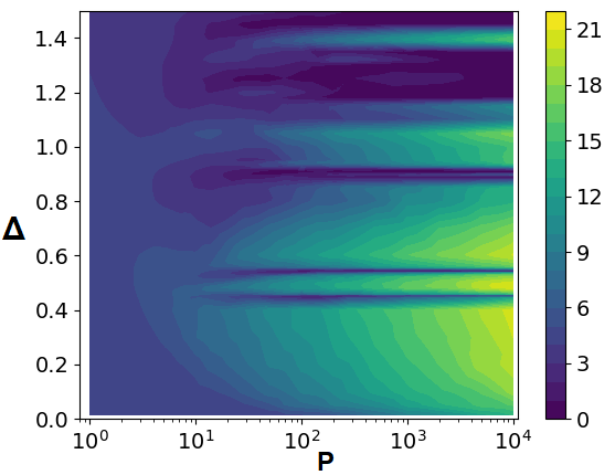
In this case, (where 13.9077 is the spectral range of this problem) due to wrap around of the eigenvalues of the cost ground and highest excited states. Below is the behavior predicted in Section 5.3, with performance at fixed improving as increases. The performance improvement is quite drastic in some cases; for instance, achieving squared overlap at requires , while at it is only .
The wrapping cost ground and maximal excited states are directly coupled by the mixer, so the redirection of the ground state to the excited state is noticeable at small . Since the expected energies of the cost wrapping states are similar for , Eq. 18 does not directly apply. However, we expect an exponential dependence on and verify this by using Eq. 19 to predict the value of at which the performance hits squared overlap, given an overlap of at . This estimates a overlap at , which is close to the true value of .
Slightly increasing restores the connection between the two Hamiltonians’ ground eigenstates - this is because the spectrum of the two Hamiltonians is so similar that the ground/maximal excited states of wrap around at before any more cost eigenvalues wrap past each other, “undoing” the altered connection between the ground eigenstates of the two Hamiltonians. The cost Hamiltonian directly couples the highest/lowest eigenstates of the mixer, so this transition is clearly visible at low , just as the first. Thus our topological perspective offers a more intuitive explanation for why performance deteriorates on such a narrow band of than the usual angle size divergence analysis.
Above this value of , due to the weak connections between the cost eigenstates produced by the mixer (and vice versa), eigenvalues of indirectly-connected states wrapping around do not result in gaps that are noticeable at this scale. Eventually, above , enough significant gaps from avoided crossings due to wrap-around have emerged that performance completely deteriorates.
7 General Schedules and Problem Size Scaling
This section shows how the explanations of Section 5 apply to additional cases of performance diagrams.
7.1 General schedules with gradually changing angles
The previous two sections illustrated how the small-angle approximation, eigenstate connections for in the adiabatic limit and small eigenvalue gaps explain performance diagrams for QAOA using the linear ramp of Eq. (4). This section generalizes these explanations to other schedules with gradually changing angles. This is of general interest as there is strong numerical evidence that optimized QAOA protocols approach an asymptotic continuous limit with large Zhou et al. 2020; Pagano et al. 2020; Brady et al. 2021.
One set of results applies to schedules in the discrete adiabatic limit. Schedules with gradually changing as defined in Section 2 correspond to discrete samplings of continuous paths in parameter space. Section 4.3.5 describes how the mixer and cost eigenstates connected by continuous paths through parameter space are determined entirely by the initial and final parameter values along that path (assuming the path does not pass through degeneracies). Applying the discrete adiabatic theorem, Section 5.2 showed which cost eigenstate the QAOA state approaches for , based only on and . Specifically, the initial eigenstate determines the cost eigenstate that QAOA produces. For small angles, QAOA can be regarded as a first-order Trotter approximation to annealing Kocia et al. 2022. One application of this generality of our approach is to analyze convergence of this approximation. In particular, fixed time-step, first-order Trotterizations of a continuous anneal correspond to fixed- paths in our parameter space. Therefore, for a fixed choice of gapped, bounded Hamiltonians and continuous schedule sampled from to produce gradually changing angles, there exists a time step corresponding to above which the product sequence of unitaries is guaranteed to fail to approximate continuous annealing.
Our results also apply to schedules with gradually changing angles where the difference between consecutive angles is not small enough to produce behavior close to that of the discrete adiabatic limit. Section 5.4 explains whether QAOA along a continuous path through parameter space follows a particular eigenvector swap, based on the gaps encountered along the path. In particular, to find the effects of gaps from wrap-arounds on nonlinear paths, it is enough to alter the calculus relative to in Appendices C.1 and C.2 to , allowing an application of our analysis to nonlinear paths (since the location and emergence of gaps can be easily translated from the parameterization in this paper). The discrete Landau-Zener approach is helpful in analyzing diabatic transitions at avoided crossings near isolated degeneracies in parameter space, not just the ones at the edges. For avoided crossings in this setting, the formula is easier to use than the general formula of the Discrete Adiabatic Theorem in (Costa et al. 2021, Theorem 3).
Unlike the discrete adiabatic theorem and Landau-Zener formula, the small-angle framework applied in Section 5.3 does not depend on the continuity of the parameter schedule and in some cases can be applied to small . Thus the small-angle analysis, which applies to the lower portion of performance diagrams, generalizes beyond schedules with gradually changing angles.
7.2 Sparse Local Constraint Satisfaction Problems: Performance Diagram and Problem Size
The performance diagrams and discussion of their properties summarized in Section 5.5 focus on QAOA performance as a function of and for a fixed problem. This section discusses how the behaviors scale with problem size for the -mixer and typical cases of sparse local-constraint satisfaction problems, i.e., problems where each constraint deals with at most some constant number of variables and each variable appears in at most a constant number of constraints.

Consider applying the mixer to a problem with size whose range of costs is , e.g., as is typical of random hard problems such as -SAT where the number of clauses, and hence maximum possible cost, is proportional to Kirkpatrick and Selman 1994. The largest eigenvalue of the mixer is also of this order in . Thus the first wrap around occurs at . Without loss of generality, for this discussion we suppose that the cost Hamiltonian has a larger range of eigenvalues than the mixer, so this first wrap around is due to that of the highest cost.
For such problems, Fig. 22 illustrates a possible scaling for the Ridge region. For large , Appendix A.3 shows that has constant QAOA performance, corresponding to the downward-sloping behavior of the bottom part of the Ridge region in the performance diagrams. These scaling arguments suggest the left-side of the ridge crosses with , which arises from minimizing the expected cost from the first two terms of (Hadfield et al. 2022, Theorem 4.2.1) applied to random Ising problems as a function of . indicates where this estimated lower bound intersects with the vertical axis at .
Above , for sufficiently large one reaches the adiabatic regime which has poor performance due to going to the wrong eigenstate, and so is outside the Ridge region.
For local constraint satisfaction problems, bit flips correspond to an change in cost. In particular, the highest cost state, of order , has bit flips compared to the ground state. Thus the coupling distance, defined in Section 4.4, between the highest cost and ground states is . Consequently, when the highest cost states wrap around, from Section 5.4, the at which significant deterioration occurs scales as , and thus will not be noticeable save for exponentially large even at fixed values of significantly smaller than 1.
In Appendix E.2, using the discrete Landau-Zener approximation from Section 5.4.2 and the lowest-order approximation of the gaps from Section 4.4, we estimate that when is some fixed polynomial function of , the gaps that produce some fixed squared overlap with the cost ground state first occur for just above , where
| (21) |
In particular, for large , we estimate that the wrap-around of states differing in bits from the ground state produces the gaps that predominantly contribute to an upper boundary to the right edge of the Ridge region, compared to all other wrap-arounds at , for polynomial in . Since even one such wrap-around is enough to produce this effect at or (see Appendix E.2), it does not matter that many excited states differing by bit flips might have a slower-scaling energy difference.
According to this analysis, the left and right boundaries of the Ridge region do not intersect when is large. The wrap-around with low-lying excited states with difference in cost from the ground state does not contribute to the right boundary, as they occur at higher values of . As we estimate in Appendix E.2, the wrap-around between cost or mixer states with coupling distance dominates in size over gaps occurring at smaller with greater coupling distance.
This analysis suggests the general scaling of the lower-left and upper-right fuzzy boundaries of the Ridge region. In particular, it suggests that for the class of problems used for this example, scaling the performance diagram axes by horizontally and vertically will result in similar diagrams for different , similar to overlapping behaviors seen with finite-size scaling in the context of phase transitions in combinatorial search such as satisfiability Kirkpatrick and Selman 1994. Importantly, the estimation from our analysis approximates an upper boundary to the Ridge region from just one effect (wrap-around at ) - other effects might need to be taken into account to predict the scaling of its actual location.
8 Discussion
The deterioration of QAOA performance at large angles was observed in Wurtz and Love 2022 and attributed to a large Trotter error in comparison to the (continuous) adiabatic limit. We identify a more complex phenomenon: the poor performance is not necessarily due to adiabaticity breaking down, but rather due to the change in connectivity between initial and final eigenstates. Our application of the discrete adiabatic theorem to schedules with gradually changing angles shows QAOA convergence Binkowski et al. 2023 and supplements analysis of digitized continuous drives Kocia et al. 2022; Hatomura 2023.
Our discussion indicates the location, i.e., ranges of and , of the Ridge region. An open question is the absolute performance of QAOA on the ridge. Numerical observations of the performance diagrams indicate performance on the ridge just above is comparable to that for small and much larger , but it remains to be seen how this behavior scales with larger problem sizes.

In particular, there may be small gaps among low-energy states that occur at values of other than the location of the gap in the highest-energy wrap around just above . Then, the absolute performance in the Ridge region might be low, as the state vector fails to go to the ground state eigenvector at small due to these other small gaps. Fig. 23 illustrates this behavior with a three-qubit example. Here, is slightly above and so there is a small eigenvalue gap near from wrap-around which is comparable in size to the eigenvalue gap between the ground and low-lying energies. Consequently, absolute performance on the QAOA ridge is limited by the gap from wrap-around for problems whose overall minimum gap is at (prior numerical investigation has found this to commonly be the case for chemistry problems Kremenetski et al. 2021b as seen in Section 6.2) and for problems where the gap with low-lying eigenstates is not as small as the gap formed from wrap-around (generically, this is true for sufficiently close to ). Therefore, another important follow-up is determining the typical performance on the ridge for different classes of problems. Further, the qualitative argument used to identify the location of the left Ridge region in the performance diagram is based on the an extrapolation of (Hadfield et al. 2022, Theorem 4.2.1) to angle sizes where higher-order terms are not necessarily small. A direction for future work here is to numerically test the applicability of this analysis to various classes of problems.
Another promising direction for future work is utilizing our approach to aid the design of schedules for low-depth circuits, which is of interest because noise in the implementation of QAOA on hardware can significantly degrade performance as the depth of the circuit grows Marshall et al. 2020; Xue et al. 2019. One could use the topological perspective to construct nonlinear schedules that exploit the structure of multiple wrap-arounds, i.e., large steps to avoid tracking swapping eigenvectors through gaps and small steps to follow eigenvectors through gaps, while using the discrete Landau-Zener approach (potentially applying discretized versions of current multi-state models Sinitsyn 2013; Lin and Sinitsyn 2014) to estimate parameter regions that have low or high diabatic transitions to the ground state at a particular depth. This could potentially allow for shortcuts to adiabatic behavior Campbell and Deffner 2017; Guéry-Odelin et al. 2019; Hegade et al. 2021. Even simpler design improvements are possible - as argued and observed numerically in our work, it is often possible to reduce the circuit depth , while increasing the angle size , with only marginal sacrifice in QAOA performance.
Another observation from our work is that judiciously picking the start and endpoints in parameter space provides an alternative means of state preparation. Starting with one cost eigenstate above an isolated degeneracy at , then taking an open half-tour around the degeneracy leads to a different eigenstate. In the cases where the highest cost excited state is easy to identify and prepare (as is the case for many Ising instances Lucas 2014), this leads to a version of QAOA where the mixer is not required to have an easy-to-prepare ground state and can be optimized to reflect structure of the cost problem. Exploiting such structure might lead to advancements Bennett et al. 1997, but whether such a protocol can improve on traditional approaches requires further investigation.
Conclusion.
In this work we have presented a new lens of analysis for QAOA circuits with gradually varying unitaries. Using the discrete adiabatic theorem, we recover the usual expected behavior at sufficiently small angles corresponding to Trotterized annealing, as well as capture the fundamentally different behavior leading to novel phenomena due to the wrap-around of unitary eigenvalues for larger angles. The latter results in changing connections between cost and mixer Hamiltonian eigenstates and diabatic transitions at small gaps due to these wrap-arounds. We have used this and other techniques such as perturbation theory to explain a surprising qualitative generality in QAOA performance diagrams from optimization to chemistry problems. Our findings represent a hitherto unexplored perspective on QAOA which carries implications for parameter schedule design, limitations of the annealing perspective on QAOA, and performance characterization.
Acknowledgments
We are grateful for support from NASA Ames Research Center. We acknowledge funding from the NASA ARMD Transformational Tools and Technology (TTT) Project. Part of this work is funded by U.S. Department of Energy, Office of Science, National Quantum Information Science Research Centers, Co-Design Center for Quantum Advantage under Contract No. DE-SC0012704. VK, TH, and SH were supported by the NASA Academic Mission Services, Contract No. NNA16BD14C. AA is supported by Yoichiro Nambu Graduate Fellowship courtesy of Department of Physics, University of Chicago. Calculations were performed as part of the XSEDE computational Project No. TG-MCA93S030 on Bridges-2 at the Pittsburgh supercomputer center. We also would like to thank Lucas Brady, Carlos Mejuto Zaera, Ruslan Shaydulin, Thomas Watts, Haoran Lu, Alexander Avdoshkin, and Andrew Yates for providing feedback on earlier drafts of this paper.
References
- Farhi et al. (2014) E. Farhi, J. Goldstone, and S. Gutmann, A Quantum Approximate Optimization Algorithm, arXiv e-prints (2014), arXiv:1411.4028 [quant-ph] .
- Hadfield et al. (2019) S. Hadfield, Z. Wang, B. O’gorman, E. G. Rieffel, D. Venturelli, and R. Biswas, From the quantum approximate optimization algorithm to a quantum alternating operator ansatz, Algorithms 12, 34 (2019).
- Ho and Hsieh (2019) W. W. Ho and T. H. Hsieh, Efficient variational simulation of non-trivial quantum states, SciPost Physics 6, 029 (2019).
- Kremenetski et al. (2021a) V. Kremenetski, T. Hogg, S. Hadfield, S. J. Cotton, and N. M. Tubman, Quantum alternating operator ansatz (QAOA) phase diagrams and applications for quantum chemistry, arXiv preprint arXiv:2108.13056 (2021a).
- Farhi and Harrow (2016) E. Farhi and A. W. Harrow, Quantum supremacy through the quantum approximate optimization algorithm, arXiv preprint arXiv:1602.07674 (2016).
- Wang et al. (2018) Z. Wang, S. Hadfield, Z. Jiang, and E. G. Rieffel, Quantum approximate optimization algorithm for maxcut: A fermionic view, Physical Review A 97, 022304 (2018).
- Wurtz and Love (2021) J. Wurtz and P. Love, Maxcut quantum approximate optimization algorithm performance guarantees for , Phys. Rev. A 103, 042612 (2021).
- Vikstål et al. (2020) P. Vikstål, M. Grönkvist, M. Svensson, M. Andersson, G. Johansson, and G. Ferrini, Applying the quantum approximate optimization algorithm to the tail-assignment problem, Phys. Rev. Applied 14, 034009 (2020).
- Díez-Valle et al. (2022) P. Díez-Valle, D. Porras, and J. José García-Ripoll, QAOA pseudo-Boltzmann states, arXiv e-prints (2022), arXiv:2201.03358 [quant-ph] .
- Akshay et al. (2022) V. Akshay, H. Philathong, E. Campos, D. Rabinovich, I. Zacharov, X.-M. Zhang, and J. D. Biamonte, Circuit depth scaling for quantum approximate optimization, Phys. Rev. A 106, 042438 (2022).
- Streif and Leib (2019) M. Streif and M. Leib, Comparison of QAOA with Quantum and Simulated Annealing, arXiv e-prints (2019), arXiv:1901.01903 [quant-ph] .
- Jiang et al. (2017) Z. Jiang, E. G. Rieffel, and Z. Wang, Near-optimal quantum circuit for Grover’s unstructured search using a transverse field, Phys. Rev. A 95, 062317 (2017).
- Kim et al. (2021) J. Kim, J. Kim, and D. Rosa, Universal effectiveness of high-depth circuits in variational eigenproblems, Phys. Rev. Res. 3, 023203 (2021).
- Koßmann et al. (2022) G. Koßmann, L. Binkowski, L. van Luijk, T. Ziegler, and R. Schwonnek, Deep-Circuit QAOA, arXiv e-prints (2022), arXiv:2210.12406 [quant-ph] .
- Zhou et al. (2020) L. Zhou, S.-T. Wang, S. Choi, H. Pichler, and M. D. Lukin, Quantum approximate optimization algorithm: Performance, mechanism, and implementation on near-term devices, Phys. Rev. X 10, 021067 (2020).
- Leng et al. (2022) J. Leng, Y. Peng, Y.-L. Qiao, M. Lin, and X. Wu, Differentiable Analog Quantum Computing for Optimization and Control, arXiv e-prints (2022), arXiv:2210.15812 [quant-ph] .
- Wurtz and Lykov (2021) J. Wurtz and D. Lykov, The fixed angle conjecture for qaoa on regular maxcut graphs, arXiv preprint arXiv:2107.00677 (2021).
- Brady et al. (2021) L. T. Brady, C. L. Baldwin, A. Bapat, Y. Kharkov, and A. V. Gorshkov, Optimal protocols in quantum annealing and quantum approximate optimization algorithm problems, Phys. Rev. Lett. 126, 070505 (2021).
- Kocia et al. (2022) L. Kocia, F. A. Calderon-Vargas, M. D. Grace, A. B. Magann, J. B. Larsen, A. D. Baczewski, and M. Sarovar, Digital adiabatic state preparation error scales better than you might expect, arXiv e-prints (2022), arXiv:2209.06242 [quant-ph] .
- Sack and Serbyn (2021a) S. H. Sack and M. Serbyn, Quantum annealing initialization of the quantum approximate optimization algorithm, Quantum 5, 491 (2021a).
- Pelofske et al. (2023) E. Pelofske, A. Bärtschi, and S. Eidenbenz, Quantum Annealing vs. QAOA: 127 Qubit Higher-Order Ising Problems on NISQ Computers, arXiv e-prints (2023), arXiv:2301.00520 [quant-ph] .
- Dranov et al. (1998) A. Dranov, J. Kellendonk, and R. Seiler, Discrete time adiabatic theorems for quantum mechanical systems, J. of Mathematical Physics 39, 1340 (1998).
- Cheon et al. (2009) T. Cheon, A. Tanaka, and S. W. Kim, Exotic quantum holonomy in hamiltonian systems, Physics Letters A 374, 144 (2009), arXiv:0909.2033 .
- Berry (1984) M. V. Berry, Quantal phase factors accompanying adiabatic changes, Proceedings of the Royal Society of London. A. Mathematical and Physical Sciences 392, 45 (1984).
- Wilczek and Zee (1984) F. Wilczek and A. Zee, Appearance of gauge structure in simple dynamical systems, Physical Review Letters 52, 2111 (1984).
- Willsch et al. (2020) M. Willsch, D. Willsch, F. Jin, H. De Raedt, and K. Michielsen, Benchmarking the quantum approximate optimization algorithm, Quantum Inf. Process. 19, 197 (2020).
- Hogg (2000) T. Hogg, Quantum search heuristics, Physical Review A 61, 052311 (2000).
- Crooks (2018) G. E. Crooks, Performance of the Quantum Approximate Optimization Algorithm on the Maximum Cut Problem, arXiv e-prints (2018), arXiv:1811.08419 [quant-ph] .
- Bigan Mbeng et al. (2019) G. Bigan Mbeng, R. Fazio, and G. Santoro, Quantum Annealing: a journey through Digitalization, Control, and hybrid Quantum Variational schemes, arXiv e-prints (2019), arXiv:1906.08948 [quant-ph] .
- Shaydulin et al. (2021) R. Shaydulin, S. Hadfield, T. Hogg, and I. Safro, Classical symmetries and the Quantum Approximate Optimization Algorithm, Quantum Information Processing 20, 359 (2021).
- Sack and Serbyn (2021b) S. H. Sack and M. Serbyn, Quantum annealing initialization of the quantum approximate optimization algorithm, Quantum 5, 491 (2021b).
- Streif and Leib (2020) M. Streif and M. Leib, Training the quantum approximate optimization algorithm without access to a quantum processing unit, Quantum Science and Technology 5, 034008 (2020).
- McClean et al. (2018) J. R. McClean, S. Boixo, V. N. Smelyanskiy, R. Babbush, and H. Neven, Barren plateaus in quantum neural network training landscapes, Nature Communications 9, 4812 (2018).
- (34) In Kremenetski et al. 2021a the performance diagrams are also referred to as “QAOA phase diagrams”.
- Costa et al. (2021) P. C. S. Costa, D. An, Y. R. Sanders, Y. Su, R. Babbush, and D. W. Berry, Optimal scaling quantum linear systems solver via discrete adiabatic theorem, arXiv e-prints (2021), arXiv:2111.08152 [quant-ph] .
- Hogg (2003) T. Hogg, Adiabatic quantum computing for random satisfiability problems, Physical Review A 67, 022314 (2003), arXiv:quant-ph/0206059 .
- Tanaka (2011) A. Tanaka, Adiabatic theorem for discrete time evolution, J. of the Physical Society of Japan 80, 125002 (2011), arXiv:1107.2989 .
- Sakurai and Napolitano (2017) J. J. Sakurai and J. Napolitano, Modern Quantum Mechanics, 2nd ed. (Cambridge University Press, 2017).
- Albash and Lidar (2018) T. Albash and D. A. Lidar, Adiabatic quantum computation, Reviews of Modern Physics 90, 015002 (2018), arXiv:1611.04471 [quant-ph] .
- Tanaka and Miyamoto (2007) A. Tanaka and M. Miyamoto, Quasienergy anholonomy and its application to adiabatic quantum state manipulation, Phys. Rev. Lett. 98, 160407 (2007).
- Miyamoto and Tanaka (2007) M. Miyamoto and A. Tanaka, Cheon’s anholonomies in floquet operators, Phys. Rev. A 76, 042115 (2007).
- Shiff (1968) L. Shiff, Quantum Mechanics, 3rd ed. (McGraw-Hill, New York, 1968).
- Ding et al. (2022) K. Ding, C. Fang, and G. Ma, Non-Hermitian topology and exceptional-point geometries, Nature Reviews Physics 4, 745 (2022).
- Tanaka et al. (2014) A. Tanaka, S. W. Kim, and T. Cheon, Exotic quantum holonomy and higher-order exceptional points in quantum kicked tops, Phys. Rev. E 89, 042904 (2014).
- Cheon (1998) T. Cheon, Double spiral energy surface in one-dimensional quantum mechanics of generalized pointlike potentials, Physics Letters A 248, 285 (1998).
- Ergoktas et al. (2022) M. S. Ergoktas et al., Topological engineering of terahertz light using electrically tunable exceptional point singularities, Science 376, 184 (2022).
- Schumer et al. (2022) A. Schumer et al., Topological modes in a laser cavity through exceptional state transfer, Science 375, 884 (2022).
- Patil et al. (2021) Y. S. S. Patil, J. Höller, P. A. Henry, C. Guria, Y. Zhang, L. Jiang, N. Kralj, N. Read, and J. G. E. Harris, Measuring the knot of degeneracies and the eigenvalue braids near a third-order exceptional point, arXiv e-prints (2021), arXiv:2112.00157 [physics.optics] .
- Altshuler et al. (2009) B. Altshuler, H. Krovi, and J. Roland, Adiabatic quantum optimization fails for random instances of NP-complete problems, arXiv e-prints , arXiv:0908.2782 (2009).
- Hadfield et al. (2022) S. Hadfield, T. Hogg, and E. G. Rieffel, Analytical framework for quantum alternating operator ansätze, Quantum Science and Technology 8, 015017 (2022).
- Bravyi et al. (2020) S. Bravyi, A. Kliesch, R. Koenig, and E. Tang, Obstacles to variational quantum optimization from symmetry protection, Phys. Rev. Lett. 125, 260505 (2020).
- Hastings (2019) M. B. Hastings, Classical and Quantum Bounded Depth Approximation Algorithms, arXiv e-prints (2019), arXiv:1905.07047 [quant-ph] .
- Cohen-Tannoudji et al. (2020) C. Cohen-Tannoudji, B. Diu, and F. Laloë, Quantum mechanics. Volume 1: Basic concepts, tools, and applications, 2nd ed., edited by S. Reid Hemley, N. Ostrowsky, and D. Ostrowsky (Wiley-VCH Verlag GmbH & Co. KGaA, Weinheim, 2020).
- et. al. (2017) R. P. et. al., Psi4 1.1: An open-source electronic structure program emphasizing automation, advanced libraries, and interoperability (2017), http://cccbdb.nist.gov/ .
- Pagano et al. (2020) G. Pagano, A. Bapat, P. Becker, K. S. Collins, A. De, P. W. Hess, H. B. Kaplan, A. Kyprianidis, W. L. Tan, C. Baldwin, L. T. Brady, A. Deshpande, F. Liu, S. Jordan, A. V. Gorshkov, and C. Monroe, Quantum approximate optimization of the long-range Ising model with a trapped-ion quantum simulator, Proceedings of the National Academy of Science 117, 25396 (2020).
- Brady et al. (2021) L. T. Brady, L. Kocia, P. Bienias, A. Bapat, Y. Kharkov, and A. V. Gorshkov, Behavior of Analog Quantum Algorithms, arXiv e-prints (2021), arXiv:2107.01218 [quant-ph] .
- Kirkpatrick and Selman (1994) S. Kirkpatrick and B. Selman, Critical behavior in the satisfiability of random boolean expressions, Science 264, 1297 (1994).
- Wurtz and Love (2022) J. Wurtz and P. J. Love, Counterdiabaticity and the quantum approximate optimization algorithm, Quantum 6, 635 (2022).
- Binkowski et al. (2023) L. Binkowski, G. Koßmann, T. Ziegler, and R. Schwonnek, Elementary Proof of QAOA Convergence, arXiv e-prints , arXiv:2302.04968 (2023).
- Hatomura (2023) T. Hatomura, Scaling of errors in digitized counterdiabatic driving, arXiv e-prints (2023), arXiv:2303.04235 [quant-ph] .
- Kremenetski et al. (2021b) V. Kremenetski, C. Mejuto-Zaera, S. J. Cotton, and N. M. Tubman, Simulation of adiabatic quantum computing for molecular ground states, The Journal of Chemical Physics 155, 234106 (2021b), https://doi.org/10.1063/5.0060124 .
- Marshall et al. (2020) J. Marshall, F. Wudarski, S. Hadfield, and T. Hogg, Characterizing local noise in QAOA circuits, IOP SciNotes 1, 025208 (2020), arXiv:2002.11682 [quant-ph] .
- Xue et al. (2019) C. Xue, Z.-Y. Chen, Y.-C. Wu, and G.-P. Guo, Effects of Quantum Noise on Quantum Approximate Optimization Algorithm, arXiv e-prints (2019), arXiv:1909.02196 [quant-ph] .
- Sinitsyn (2013) N. A. Sinitsyn, Nonadiabatic transitions in exactly solvable quantum mechanical multichannel model: Role of level curvature and counterintuitive behavior, Phys. Rev. Lett. 110, 150603 (2013).
- Lin and Sinitsyn (2014) J. Lin and N. A. Sinitsyn, Exact transition probabilities in the three-state Landau-Zener-Coulomb model, Journal of Physics A Mathematical General 47, 015301 (2014).
- Campbell and Deffner (2017) S. Campbell and S. Deffner, Trade-off between speed and cost in shortcuts to adiabaticity, Phys. Rev. Lett. 118, 100601 (2017).
- Guéry-Odelin et al. (2019) D. Guéry-Odelin, A. Ruschhaupt, A. Kiely, E. Torrontegui, S. Martínez-Garaot, and J. G. Muga, Shortcuts to adiabaticity: Concepts, methods, and applications, Rev. Mod. Phys. 91, 045001 (2019).
- Hegade et al. (2021) N. N. Hegade, K. Paul, Y. Ding, M. Sanz, F. Albarrán-Arriagada, E. Solano, and X. Chen, Shortcuts to Adiabaticity in Digitized Adiabatic Quantum Computing, Physical Review Applied 15, 024038 (2021), arXiv:2009.03539 [quant-ph] .
- Lucas (2014) A. Lucas, Ising formulations of many NP problems, Frontiers in Physics 2, 10.3389/fphy.2014.00005 (2014).
- Bennett et al. (1997) C. H. Bennett, E. Bernstein, G. Brassard, and U. Vazirani, Strengths and weaknesses of quantum computing, SIAM Journal on Computing 26, 1510 (1997), https://doi.org/10.1137/S0097539796300933 .
- Kato (1976) T. Kato, Perturbation theory for linear operators; 2nd ed., Grundlehren der mathematischen Wissenschaften : a series of comprehensive studies in mathematics (Springer, Berlin, 1976).
- Feynman (1939) R. P. Feynman, Forces in molecules, Phys. Rev. 56, 340 (1939).
- Wittig (2005) C. Wittig, The Landau-Zener formula, The Journal of Physical Chemistry B 109, 8428 (2005), pMID: 16851989, https://doi.org/10.1021/jp040627u .
- Erdos and Renyi (1960) P. Erdos and A. Renyi, On the evolution of random graphs, Publ. Math. Inst. Hungary. Acad. Sci. 5, 17 (1960).
- (75) DLMF, NIST Digital Library of Mathematical Functions, http://dlmf.nist.gov/, Release 1.1.8 of 2022-12-15, f. W. J. Olver, A. B. Olde Daalhuis, D. W. Lozier, B. I. Schneider, R. F. Boisvert, C. W. Clark, B. R. Miller, B. V. Saunders, H. S. Cohl, and M. A. McClain, eds.
- Bollobás (2001) B. Bollobás, Random graphs, 2nd ed., Cambridge studies in advanced mathematics No. 73 (Cambridge University Press, 2001).
- Bogdanowicz (2009) Z. R. Bogdanowicz, Undirected simple connected graphs with minimum number of spanning trees, Discrete Mathematics 309, 3074 (2009).
Appendix
Appendix A Application of QAOA small-angle analysis
The results for QAOA in the small-parameter regime of (Hadfield et al. 2022, Theorem 4.2.1) describe behavior at the bottom of the performance diagram. This theorem expresses the expected cost of the final QAOA state as a series in polynomials of the QAOA angles, with coefficients determined by initial state expectation values of operators derived from the cost function via commutators Hadfield et al. 2022. For level- QAOA, to leading-order
| (22) |
where the terms not shown to the right are proportional to increasingly higher order products of the , with the next nonzero contribution proportional to a quartic polynomial of the QAOA angles.
A.1 QAOA schedules
For the ramp schedules of Eq. (4), the parameter polynomials of (Hadfield et al. 2022, Theorem 4.2.1) are functions of and . The angle sum appearing in the leading order term is
| (23) |
The small-angle analysis applies to arbitrary parameter schedules. In particular, (Hadfield et al. 2022, Remark 4.2.1) indicates the angle sum terms scale as powers of in the same way as the ramp when is interpreted as a characteristic magnitude of the angles. Thus the dependence on and in the theorem does not depend on specific details of the QAOA schedule, thereby indicating why the observed QAOA performance diagram behavior is generic in the regimes of validity of (Hadfield et al. 2022, Theorem 4.2.1), in particular when (for fixed problem size).
A.2 Ising problem
Finding the ground state of a Hamiltonian is a minimization problem, so we use as the mixer, so the initial uniform superposition is the ground state of the mixer. This contrasts with the use of the mixer in Hadfield et al. 2022. This change of sign of mixer is equivalent to changing the sign of instead. In applying this theorem to finding the ground state of the Ising problem, we make this sign change in the angle sums.
For the Ising Hamiltonian of Eq. (20), the leading-order correction to of (Hadfield et al. 2022, Theorem 4.2.1) is
| (24) |
The random Ising problems considered here have , so averaging over this problem class gives
| (25) |
which equals for large ,. A similar evaluation of the angle sums and costs involved in the second term of (Hadfield et al. 2022, Theorem 4.2.1) for large gives .
These expressions allow generalizing the range of validity of this series expansion beyond for fixed and a given problem (hence fixed ) discussed in Hadfield et al. 2022. Specifically, the second term is small compared to the first when .
The first term is negative, indicating decreases, i.e., QAOA performance improves, when moving from the lower left toward the upper right of the diagram, until the second, and higher, terms become important for and lead to increasing . This suggests the Ridge region in the performance diagram occurs for or larger. On the other hand, gives the adiabatic limit, which gives low performance above .
A similar analysis applies to sparsely connected Ising problems that correspond to local CSPs discussed in Section 7.2. One such class of problems is when each pair of spins is independently connected with probability with a fixed constant, independent of . Thus, on average, a spin is connected to other spins. The couplings for connected spins are randomly selected in the same way as for the fully connected case described in Section 6.1.
For the small-angle analysis, the sparse Ising problem only changes the expectation values of the coupling appearing in the cost operators, e.g., in Eq. (24). In particular, and, for large , the leading-order term is . Similarly, the second term of (Hadfield et al. 2022, Theorem 4.2.1) is . Both these terms are linear in , and the second term is small compared to the first when . This indicates a lower bound for the ridge region of these sparsely connected problems occurs with .
A.3 Scaling from small-angle analysis
Any problem whose cost operator expectations and maximum energy depending on in the same way as the Ising example will have the same scaling for the location of the Ridge region in terms of as the Ising example. This includes any QUBO whose cost coefficients are independent of (Hadfield et al. 2022, Lemma B.0.2).
Moreover, the angle sums in the series expansion of (Hadfield et al. 2022, Theorem 4.2.1) are proportional to powers of for large (e.g., the angle sum given in Appendix A.1). For higher order terms to be small requires , rather than just used in Hadfield et al. 2022 in the context of fixed . Thus, for large , has constant QAOA performance, corresponding to the downward-sloping behavior of the Ridge region for small-to-intermediate in the performance diagrams.
The schematic scaling shown in Fig. 22 is given by combining these observations for sparsely connected problems, and extrapolating the small-angle series from so small that QAOA operators are close to the identity so the QAOA output state is close to the initial state. This emphasizes the qualitative behavior for moderately large .
For such problems, as discussed in Section 7.2, is of order . This suggests the Ridge region occurs when is at least of order , i.e., is at least of order .
A consequence of this discussion of the size of the terms in (Hadfield et al. 2022, Theorem 4.2.1) is that is not large enough for QAOA to reach the Ridge region since we have at most to avoid wrap-around so is then at most of order , which is small compared to 1. Thus the first term dominates, indicating performance increases with increasing beyond so these parameters are below the Ridge region.
For problems whose costs scale with differently than the Ising example, a similar analysis can use the corresponding scaling of expectations of cost operators appearing in (Hadfield et al. 2022, Theorem 4.2.1), and the dependence of the maximum energy to determine scaling of . Using these scaling behaviors will give corresponding estimates for the location of the Ridge region.
Specifically, the small-angle analysis can indicate the scaling of cost Hamiltonians that have different connectivity among the problem variables than the fully and sparsely-connected cases discussed here. For instance, a local Hamiltonian, where each variable only interacts with other variables instead of fully connected interactions, will have substantially fewer terms in the cost expectations leading to slower growth with . For problems with pairwise interactions among variables, (Hadfield et al. 2022, Lemma B.0.2) gives the cost expectations in terms of sums over the interaction strengths. Similarly, (Hadfield et al. 2022, Lemma 2.5.3) includes the generalization to interactions among triples of variables, which is relevant for the scaling of performance diagrams for 3-SAT which have qualitatively similar features to those seen with pairwise interactions Kremenetski et al. 2021a. The number of nonzero terms in these sums determine their scaling with respect to problem size .
A.4 Molecular ground state problems
Our QAOA construction for the electronic structure problem Kremenetski et al. 2021a is also considered in (Hadfield et al. 2022, Sec. 5.3). As indicated there, it is relatively straightforward to extend the result and proof of (Hadfield et al. 2022, Theorem 4.2.1) to the quantum chemistry setting, which results in a similar term at leading order to the Ising case.
Appendix B Results for isolated degeneracies
Here we provide supporting results for the claims regarding isolated degeneracies of Section 4.
B.1 Formula for gap from wrap-around of two non-degenerate eigenstates
We derive a perturbative formula for the size of the gap resulting from wrap-around of two non-degenerate cost eigenstates at based on and the couplings of cost eigenstates by the mixer. It may be trivially modified to account for wrap-around at .
B.1.1 Formula for gap size
We first introduce some helpful definitions.
Definition.
Two cost eigenstates are said to be “coupled” by the mixer if there exists an ordered tuple of cost eigenstates such that
| (26) |
We call such this set a “coupling path”, and the cardinality of this set the “length” of the path.
For example, with the -mixer, states and have a coupling path of length three. This is not the only coupling path between the two states, others exist of the same length (e.g., ) or different length (e.g., ).
Definition.
Two cost eigenstates are said to be “k-coupled” by the mixer if the shortest coupling path between them is of length .
For the -mixer example, the states and are 3-coupled, because the X-mixer directly couples two bitstrings with a Hamming distance of one, so all the shortest coupling paths between these two bitstrings have a length of 3. In general, for the case of the -mixer and computational () basis, states whose bitstrings have a Hamming distance of are -coupled. We now recursively define a multivariate polynomial:
| (27) |
The first few orders of this polynomial are shown in Table 1.
Gap Formula: Let such that for exactly two distinct, non-degenerate energies of and suppose the corresponding eigenstates are -coupled by the mixer. Then, for a path at , and using Eq. 29, the gap magnitude from the avoided crossing due to wrap-around is
| (28) |
if
We introduce notation:
| (29) |
where are cost eigenstates. In practice, for many common mixers (zero diagonals), which simplifies our formulas. Next, we define for the -th term in some fixed coupling path
| (30) |
Finally, we define an “effective” coupling between states as:
| (31) |
where the sum is over all coupling paths between the states.
If , the degeneracy at is guaranteed to be isolated. As this is generically the case (though see examples of exceptions in Appendix E.1), it follows that the degeneracy is generically isolated and the resulting gap from wrap-around goes as as . That is, the gap size shrinks exponentially with coupling distance. Further, the size of the resulting gap depends to lowest order only on the energies of the intermediate coupling states, so if , the resulting gap goes as as , and it is not a guarantee that the degeneracy at is continuous (not isolated). Finally, while is difficult to compute in general, it depends only on and , allowing a characterization of how quickly the gap grows as increases above . Also, given the simple recursive formula in Eq.27 which we use to determine , this formula is simpler than conventional perturbation theory Sakurai and Napolitano 2017; Kato 1976 when becomes large. An area of future work is to compute “average” values of and its scaling with for different families of mixer/cost Hamiltonians, as is done in Appendix E. In deriving the formula, we also get a first-order estimate for the gap location in a fixed- path, satisfying .
| k=1 | |
|---|---|
| k=2 | |
| k=3 | |
| k=4 | |
| k=5 |
B.1.2 Deriving Gap Formula
To derive the gap formula, Eq. 28, consider wrap-around that takes place at such that for non-degenerate cost eigenstates . Suppose that at the gap from avoided crossing due to wrap-around occurs at , then without loss of generality the QAOA unitary (as defined in Eq. 5) may be expressed as:
where and are the eigenvalues and eigenvectors respectively of the QAOA unitary, and are the eigenvectors involved in the eigenvector swap. These eigenvectors and the gap depend on . We define distance in parameter space from the point of degeneracy at . The difference between and
| (32) |
goes as , . From perturbation theory Kato 1976, the difference between and the nearest eigenvector of goes as , as does the difference between the eigenvalues of and the nearest eigenvalues of . As discussed in Section 4.3, and lie predominantly within the subspace spanned by and , though and can have magnitude of overlap with other . Since , we cannot simply compute the submatrix of on and , as the order of the gap size could be of the same order as overlap with the other eigenvectors of . To resolve this, we introduce the “residual matrix” of a unitary , :
| (33) |
By choosing , we have:
| (34) |
The remaining term is negligible provided that . As each is perturbatively within of some eigenvalue of , it is from here that the requirement of being non-degenerate with other eigenstates of originates, and that we expect our gap formula from Eq. 28 to break down when the predicted eigenvalue is of the same order as separation of of other eigenvalues of .
Now, where is orthogonal to and . Consequently, we have:
| (35) |
| (36) |
and
| (37) |
Perturbation theory implies that the leading order change comes from the diagonal terms. Therefore, for for fixed , the choice of gap is minimized when we choose such that the first-order-in- components of and vanish. Computing these values will yield a first-order approximation of the gap location. First, we enforce that both terms cancel out their first order in contributions:
with an analogous equation holding for . Thus, by solving the following equation
we obtain a relation between and
| (38) |
Here, are given by Eq. 29. This provides us with a first-order estimate of the gap location from the avoided crossing. As an aside, if we regard the “unperturbed” energies in the computational basis near as being given by a slightly more accurate approximation would replace with in Eq. 38. However, we will proceed with this first-order estimate as we are interested in the lowest-order estimate for the gap size. This approximation is only valid in the regime where is large compared to .
The terms appearing in Eq. 37 are not independent since . Thus for fixed , we try to choose and such that any one of them is minimized (to lowest order in , is fixed with ). We will now focus on term
Since are -coupled to each other, we must choose at least total powers of from the above product for the contribution to the product to be non-zero. Since we’re working in the eigenbasis of , the terms are diagonal and we only have to consider the terms coming from the Taylor expansion of . Therefore, the lowest power in contributions to this term come from only considering total powers of coming entirely from powers of ,
To identify the relevant terms, we fix a particular coupling path . Every time we apply a term from the product to the ket on the right, we choose whether to apply or a power of to hop further along the coupling path to . Crucially, since each term in the product commutes with every other term, we can order the however we want when computing the contributions of each set of hops along each coupling path (e.g. hops of from the coupling path ). A hop over states would require choosing a power of the mixer.
Recall that each is within of an eigenvalue of and that all states on our coupling paths are eigenstates of . Exploiting the freedom in ordering, to evaluate the contribution of hops along indices of a particular coupling path , we order the ’s to apply them in the order that the hops visit the states with the closest eigenvalues. This forces us to choose to hop further along the path for the multiples that we encounter (otherwise we get an extra contribution from , which we ignore as we are only considering the lowest order terms in ), giving us a multiple along the way for the state visited. After that, our path has already arrived at and thereafter we pick only , giving us, to lowest order in , multiples of form where are the energies of the states not visited in the hops over the coupling path. In other words, for a fixed coupling path , (and letting ), the contribution is:
where the summation is over all ordered subsets of and is the hopping distance in between consecutive elements of . Dividing out from Eq.36 gives:
We simplify this expression by noting that and by organizing the summation recursively as sums of all hops starting with plus all those starting with , etc., giving:
with function as defined in Eq. 27. Therefore we have
The resulting expression, to lowest order, only depends on . Therefore, for a given , we have a degree of freedom to optimize through varying . Note that from Eq. 37, the gap is minimized when , i.e. when the swap of eigenvectors is half-way through. It’s important to note that fixing and varying which (we know to be of ) to minimize the gap size at doesn’t necessarily yield the same gap as then fixing and varying , unless that minimum already happens to be very close to . In this latter case, the numerators will be approximately the same and therefore the denominators will be both approximately (this is as large as they can get). From perturbation theory, we expect the exchange of eigenvectors to take place over interval at fixed for , and since our is in the middle of the exchange, the optimal for is approximately . Appendix C.1, shows this interval goes as . Thus, for , we can approximate the denominator as , and the minimum gap location of the avoided crossing coincides with the middle of the eigenvector swap in the perturbative limit, i.e. the exchange of eigenvectors occurs approximately symmetrically about the avoided crossing from wrap-around. For a different approach is required, as shown in Appendix B.1.3.
B.1.3 Special Case: k=1
When the wrapping states and are directly coupled, we can compute the gap from the submatrix of on the subspace. To lowest order in , the terms are:
We define for the ease of notation. The eigenvalues of this submatrix of are approximately and so by calculating the minimum gap between the eigenvalues of this residual matrix (fixing and changing to minimize the gap), we approximate the overall gap from the avoided crossing due to wrap-around. Dividing out the common product term and the imaginary unit, the gap between eigenvalues of a two-by-two matrix with diagonals and equal off-diagonals is given by , so that
B.2 Feasible regions for intermediate degeneracies
In Section 4.4 we mention that no isolated degeneracies due to wrap-around occur at below the at which the first wrap-around occurs at (from the previous section, generically we have ). This appendix proves this statement. The proof also shows that, below , the eigenvalue curves connecting maximal excited eigenvalues are always closest to eigenvalue curves connecting ground eigenvalues at the edges , implying that below , no swaps take place either, i.e. no narrow avoided crossings between the two curves.
Theorem 1.
Let be the smallest value of at which a pair of eigenvalues of wraps around at either or . Then, if is a point of isolated degeneracy due to wrap-around between the two eigenvalues, with , we must have
Proof: This is trivially true for and we will prove it holds for as well. To do so, we first recall the definition of the QAOA Hamiltonian, , given by Eq. 13, choosing to be equal to at , equal to at , and to have continuous eigenvalues in between. Prior to the wrap-around of eigenvalues (i.e. when we can choose a branch cut such that the eigenvalue curves do not pass through the cut boundaries), this can always be done.
Due to ordering and geometry, the first eigenvalue curves of that interact with each other due to wrap-around are the eigenvalue curves connecting maximal excited eigenvalues and the eigenvalue curves connecting ground eigenvalues. Therefore, if and , then has either a lower ground state energy than and , or a higher maximal energy than and . We shall show that this is impossible.
First, we shift the spectra of and for convenience so that, for each Hamiltonian, respectively, the highest and lowest energies are equal in magnitude and opposite in sign. Note that this is equivalent to multiplying by a global phase, which cannot affect the formation of degeneracies. In this setting, will have a lower minimal energy or higher maximal energy if and only if it has an energy with a greater magnitude than that of any energy of or .
Let be the largest eigenvalue of at , and let be the corresponding eigenvector (choice of eigenvector is continuous in the absence of degeneracies). Finally, we define as the largest magnitude of any eigenvalue of the mixer and as the largest magnitude of any eigenvalue of the cost, and recall that .
Suppose and share either a minimal or a maximal eigenspace. Then the maximum magnitude energy of both and is (since those eigenspaces are simultaneously diagonalizable) and therefore cannot be larger in magnitude than . We will now consider the case where and do not share ground/highest excited eigenspaces. In this instance, when .
To begin with, we take the partial derivative with respect to of both sides Eq.13:
Dividing out the imaginary constant, and substituting in gives us:
We simplify this expression using the Hellmann-Feynmann Theorem Feynman 1939 and defining and :
Note that the matrix elements of depend analytically on , and therefore so do the coefficients of ’s characteristic polynomial. From this, we know the eigenvalues of vary continuously with . From the Implicit Function Theorem, the eigenvalue is also a continuously differentiable function of the characteristic polynomial coefficients (and thus of ) if it is non-degenerate. Since we consider the eigenvalue near an isolated degeneracy, with and not sharing a maximal eigenspace, for any fixed and choice of there must exist some open interval along which is non-degenerate and hence differentiable. We suppose that we operate on such an interval moving forward. We now take the absolute value of both sides and note that the right hand side is at most the largest eigenvalue of :
| (43) |
We now use this bound for a proof by contradiction. Suppose there exist such that at for an eigenvalue for either the ground or highest excited eigenvalues of . Without loss of generality, suppose . Note that for any fixed , there must exist a smallest for which this equality is attained, since in the limit of , we have due to approximating . From now on, we fix and consider as the smallest value of where this equality is attained.
Next, we will show through a proof by contradiction that there must exist constants s.t. . Suppose that no positive lower bound exists for on any such interval. Let
Note that since is continuous,
On this same interval, by hypothesis we can find a such that
From this, we get:
| (44) |
This gives us a contradiction. So such that . Note that this derivative must be positive, since is the smallest value of where attains this large of a value. Consequently, we must have . From here, we get the final step of our proof - that
| (45) |
Since is continuous, this gives us a contradiction, since it cannot equal at .
Therefore, we cannot have a with magnitude greater than or equal to for any when and do not share a maximal eigenspace before the wrap-around at the edges or . Together with the case we’ve already considered where they do share one, this concludes the proof.
Appendix C Deriving tracking estimates and describing the performance ridge
Here we characterize the value of at which overlap with the state prepared in the discrete adiabatic limit starts increasing with increasing using estimates on the eigenvector swap interval and discretized Landau-Zener to derive equations for performance deterioration as discussed in Section 5.4.
C.1 Estimating width of interval over which eigenvector swap happens
Consider the eigenvectors of swapping along a fixed- path in parameter space. If close to , we can approximate this as a swap between cost eigenstates and , as the eigenvectors of will be very close to those of . We first derive an estimate of the length of the interval in the schedule over which a swapping eigenvector changes from having squared overlap with initial eigenvector to overlap with it. While a direct estimate of the critical discretization required to start gradually tracking the eigenvector swap is left for future work, the inverse of this interval is a rough proxy for its scaling.
Our initial approximation, as mentioned above, is that the swap happens precisely between states and (we expect this approximation to be most valid when is not too close to 0 or 1, i.e. the difference between and 0 or 1 must be above order ). We also assume that support on other cost eigenstates is negligible - this assumption is justified provided that the eigenvalue gap between the two swapping eigenvectors remains much smaller than the gaps between them and other eigenvalues. We denote the two swapping eigenvectors as follows:
| (46) |
with and . The operator restricted to the subspace of these two eigenvectors, is given by
| (47) |
with being the eigenvalue associated with . Now, we step symmetrically to the other side of the minimum gap from the avoided crossing, where the two eigenvectors will have exchanged places in relative overlap. Since the gap is formed from an avoided crossing between two locally linear spectral curves, the avoided crossing has a slant, so both eigenvalues gain an extra phase of . By symmetry, both are otherwise the same as on the other side of the gap. The operator restricted to the subspace of the two eigenvectors is therefore:
| (48) |

We take the difference between Eq. 47 and Eq. 48 using Eq. 46. The resulting contributions for and are:
| (49) |
Since is the (very small) difference between two unitary eigenvalues, it is almost entirely orthogonal to them in their vector representations (i.e. the representation of ), and so is almost entirely orthogonal to the vector representation of ). Consequently, the absolute value of each coefficient is minimized when , i.e., when the avoided crossing doesn’t have a slant. Since the avoided crossing we consider takes place near , by shifting all the energies of by some constant, we can either shift the slant further or reverse it - meaning at some intermediate energy shift, we can eliminate the slant entirely. To do so, we compute (and choose an energy shift to minimize) the following expression:
| (50) |
For , we can approximate the difference as
| (51) |
Using Eq.51, and Eq.29, we can approximate Eq.50 as
| (52) |
Recalling that we want to shift the energies of by some constant to minimize this quantity, some simple calculus shows this to be obtained for . Under this shift, the avoided crossing is no longer slanted (while the gap is unaffected as shifting the energies of the cost contributes only a global phase), so simplifying Eq.49 with and plugging in the shift to Eq.52 yields
From our main gap equation in Eq.28 and Eq.37, we can replace with . Solving for , we obtain
| (53) |
Further away from , the swap won’t take place between precisely and , but rather between eigenvectors with strong support on these two eigenvectors. To estimate the eigenvector composition outside of this avoided crossing, non-degenerate perturbation theory gives
| (54) |
where is the location of the gap. Since the eigenvector changes from first order perturbation to the operator from near take place over much larger interval than most of the swap near the avoided crossing (for ), we approximate at the gap location itself. Defining , we get a “normalized” version of the swap interval formula:
| (55) |
where is the length of the interval at fixed over which a swapping eigenvector goes from having squared overlap with to having that same squared overlap with instead. Fig. 24 shows the formula has good agreement with numerical simulation. As a perturbative formula, its accuracy is highest when it is near the value of at which wrap-around happens (Fig. 24(B) has a larger relative error due to it having smaller compared to the eight-level example, since the approximation of a symmetric swap about the minimum gap of the avoided crossing is better suited the greater is than 1). Further, the unnormalized version tends toward underestimating the interval length (it predicts a finite interval between two high overlaps that might not be attained due to swap happening between eigenvectors not exactly ), and the normalized version inevitably overestimates the interval length (it predicts an infinite interval length for a completed swap ).
Therefore, the swap only takes place over some finite interval outside of which dynamics due to first-order non-degenerate perturbation theory dominate.
C.2 Discrete Landau-Zener
The eigenvector swap occurs in the neighbourhood of the gap from wrap-around. The other eigenvalues are well-separated from those associated with the swapping eigenvectors, as illustrated in Fig. 9. Thus the dynamics in the neighbourhood of the avoided crossing can be described by an off-diagonal perturbation in the effective two-level Hamiltonian Cohen-Tannoudji et al. 2020
| (56) |
where and are the unperturbed energies of the eigenvectors near the avoided crossing which vary with , and is the size of the off-diagonal coupling. The energy gap at the avoided crossing is twice the value of . The leading order change in energy difference can be approximated by a linear function
| (57) |
where is number of steps away from the avoided crossing and the total step count and are related by Eq. 3. When the value of is large enough that the state vector follows a QAOA eigenvector, the Landau-Zener formula Wittig 2005 gives the probability of a diabatic transition between the two eigenvectors
| (58) |
In our case, we can estimate the “unperturbed” energies as the eigenvalues of the cost and mixer diagonals in the cost (mixer) eigenbasis for wrap-around at (). For wrap-around at , the energies as a function of are simply
| (59) |
| (60) |
Assuming that the wrap-around between these two eigenvalues takes place for the first time at gives
| (61) |
where are given in Eq. 29 and . This estimation of the “unperturbed” energies is only valid for not close to 1. Otherwise higher-order corrections become more relevant. Further, is half the magnitude of the perturbed gap between the eigenvalues, and so from Eq.28 is given by
| (62) |
where depends only on “normalized” Hamiltonians , and the magnitude of the product of off-diagonal coupling terms of .
From Eq. 58, the energy difference is a function of which in turn is inversely proportional to for a linear ramp and therefore the energy difference per QAOA step near the avoided crossing is given by
| (63) |
where the partial derivative is taken on either side of the avoided crossing. Using this in Eq. 58 shows that the probability has an exponential dependence on the number of steps as captured by Eq. 18
| (64) |
| (65) |
where
| (66) |
Appendix D Details for eight-level example
D.1 Computing discrete Landau-Zener formula for each wrap-around
This appendix derives the curves in Fig 18(A), which uses the Hamiltonian pair from Fig 9. The ground state, , wraps around with four excited states at over the span of considered in the plot. In particular, the states , and . Each of these, in turn. wrap around with other states, but we are only interested in the gaps from wrap-around with the ground state as those are responsible for the deteriorating performance. First we need to compute for each wrap-around. To do so, we can use the simplified expressions of Eq. 27 in Table 1 for , as we use the X-mixer rescaled by 0.5 which directly couples states with Hamming distance 1. Further, as a consequence of this mixer choice, we have from Eq. 29. The energies of the cost Hamiltonian are given by:
| (68) |
For the wrap-around between and , we have . The coupling paths we must consider are all distinct ways to get from to in three bit-flips. From Eq. 26 we have for all coupling 3-paths, and from Eq. 31, we have:
Applying Eq. 65, and defining , we have
Solving for that gives the value for this state gives the value
| (69) |
For the wrap around between and , we have and respectively. Considering all possible paths between and in two bit-flips gives:
Solving for after plugging in and the relevant constants into Eq. 65 leads to
| (70) |
| (71) |
where and . In the case we have and . By applying Eq. 67 and solving for , we obtain
| (72) |
| Wrapping Excited State | ||||
|---|---|---|---|---|
| 0.0789 | 0 | |||
| 0.125 | 0 | |||
| 0.1765 | 0 | |||
| 0.5 | 0 |
Table 2 summaries the resulting parameters.
D.2 Combined effect from all gaps
In this section, we derive the curve displayed in Fig. 18(B).
We want to estimate the value of at which the squared overlap of the QAOA output state with the ground state is 0.95. Under the assumption that is large enough for the QAOA state vector to track the eigenvectors up to the first few gaps, we get
| (73) |
with the terms given by Eqs. 69-72. For values of below the at which wrap-around with state occurs, we take . As expected, the smallest , if significantly smaller than the others, dominates the shape of the right edge of the performance ridge.
D.3 Correcting for poor tracking
Here, we derive the curve in Fig. 18(C). We approximate the squared overlap due to non-wrap-around gaps as occurring for for some unknown constant . This can be re-written as where we approximate as the at which there is a squared overlap of with the ground state at , just below . This is numerically determined to be between 14 and 15 - we use 14.5 to generate the curve. The overall formula becomes
with given by
| (74) |
We numerically scanned values of near the ansatz from Eq. 73 such that the two sides in Eq. 74 are as equal as possible to produce Fig. 18(C).
Appendix E Local-constraint satisfaction problems with the -mixer: effects of wrap-around
E.1 Exponential scaling of gap size for most wrap-arounds in this setting
In this section, we examine a special case where the scaling of the gap size from wrap-around has an exponent potentially much larger than the coupling distance between the wrapping states.
Consider a cost Hamiltonian and the two sets of qubits, and , that and respectively perform non-identity operations on. Suppose , with diagonal in the computational basis. Suppose wrap-around takes place between two cost eigenstates that differ by bit flips on a set of qubits and that . Suppose the wrapping cost eigenstates differ by energy on and by and on and respectively. Note that since , the qubits under the two Hamiltonians are separate systems, and so all changes in eigenstate connections between the mixer and must correspond to changes in eigenstate connections between the mixer and and restricted to and respectively. Consequently, the mixer eigenstate will only change its connection to the eigenstate whose eigenvalue is wrapping around at if it corresponds to a wrap-around for both and (otherwise the change will be to an eigenstate with only some or no bits flipped, i.e. to the same cost eigenstate or to a cost eigenstate with energy difference just or just ).
Now consider the setting of two cost eigenstates and wrapping around with where at most of the coupling terms are nonzero for some constant . Suppose that these eigenstates differ by bit flips on qubits with indices (different combinations of flips on these qubits form the shortest coupling path between the states by the X-mixer). Therefore, for qubits with , the single-qubit ket will be the same for all states in all of these paths, and so for the specific purpose of calculating the contribution to the gap from the energies of the states along the shortest coupling path, we can simplify every Pauli operator in as follows:
If the couplings on the flipped qubits fail to form a connected set, then the resulting “reduced” Hamiltonian can be separated into two Hamiltonians acting non-trivially on disjoint, non-empty subsets of the qubits. Since we know that in this setting a continuous degeneracy almost always forms, the contributions of all the shortest coupling paths must cancel out to zero. Therefore, the contributions of coupling paths passing only through states whose bit-flipped qubits don’t have couplings forming a connected set over the qubits must cancel out (i.e. from Eq.31 and Eq.28, and any higher order terms involving only those states must cancel as well).
Let be the size of the smallest set of qubits that (1) has the qubits subject to bitflips along the shortest coupling paths of length as elements and (2) has the couplings form a connected graph over the qubits in the set. Since the bits not in the shortest coupling path have to be flipped twice (since they don’t differ between the starting and final states), a total of bit flips are required. Consequently, the gap from the wrap-around scales as .
For local constraint satisfaction problems on logical qubits, the probability of two qubits sharing a coupling goes as for some constant . From random graph theory Erdos and Renyi 1960, we know that subgraphs of size significantly smaller than have a vanishingly small probability of being connected. From this, we can infer that almost all (though certainly not all, for an overall connected graph of couplings over all qubits) wrap-arounds involving two cost eigenstates differing by a sublinear-in-qubit-number of bit flips nevertheless have and therefore have gaps scaling exponentially in qubit number.
This analysis is useful outside of local-constraint satisfaction problems. We can consider the case where the cost and mixer Hamiltonians are both decomposed into sums of Pauli strings. In this case, if and are the wrapping cost eigenstates, then we consider a set of qubits subject to constraints that (1) the set cannot be separated into two disjoint subsets where the every Pauli string of the cost and mixer acts non-trivially on at most one of the subsets and (2) the number of mixer Pauli strings required to flip bits to go from to is minimized to some number . Then the gap from wrap-around scales as .
E.2 Performance ridge: location scaling with problem size
In this section, we justify our claim that some fixed degree of performance deterioration due to wrap-around is attained at polynomial in (the number of qubits) from wrap-around with as much as a single excited state differing by bit flips and energy from the ground state, with from Eq. 21, which we call “quasi-logarithmically distant excited states”. This forms an upper boundary at for where the right edge of the performance ridge can be for with a constant , since performance deterioration occurs past this point due to wrap-arounds at (though we cannot say what happens to performance up to this point). Since -mixer eigenstates differing by flips (i.e. ) are connected by the transitions by the terms of , this analysis applies equally to wrap-around by cost and mixer states. Further, it ought be noted that our analysis applies even to the case of with degenerate ground states, since the -mixer has a non-degenerate ground state, and so even the wrap-around of a single mixer excited state with this quasi-logarithmic coupling distance is enough to change the connection to some distant cost excited state.
We make our argument as follows. First, we show that the quasi-logarithmically distant excited states are the most distantly coupled set of states from the ground state for which, at (i.e., ) a single gap is large enough to achieve some fixed, low diabatic transition rate to the ground state at for some constant . Thereafter, we show that this result is unaffected by the a large number of very small gaps from more distant wrap-arounds, because they collectively do not result in some noticeable reduction in the diabatic transition to the ground state prior to the wrap-around of quasi-logarithmically distant excited states. That is, a “death by a thousand cuts” does not happen.
The rigor of our argument has some limitations. Firstly, we use lowest-order estimates of the gap sizes to make these conclusions. For sufficiently large , the lowest-order calculation overestimates the gap size (the eigenvalues are constrained to be on the complex unit circle) and thus our argument on the irrelevance of distant excited states remains valid. Additionally, the values of we consider are much smaller than , making the approximation reasonable. Another limitation is the estimation of a typical scaling of from Eq. 65. There is numerical evidence that this term scales exponentially with coupling distance (see Fig. 25), but this remains unproven. Finally, we assume that any higher-order transitions back to the ground state occur through several other gaps, and thus are negligible compared to the reduction in diabatic transitions to the ground state at the “diabatic” ground state eigenvalue curve’s crossings with other excited states.
E.2.1 Polynomially small gaps
For , the exponent of Eq. 65 attains a non-growing diabatic transition to the ground state at for if , where , is the coupling distance, and is some constant converting coupling distance to energy difference. Note that and the exponential-in- can be absorbed by multiplying by an overall constant. Therefore, we establish the smallest possible scaling of with respect to by solving:
| (75) |
The condition is satisfied with equality for if where is the Lambert W function DLMF. Consequently, for large , and arbitrary , . For the -mixer, and likely for the cost Hamiltonian as well, at least one excited state exists that has both a coupling distance and energy difference of . Without loss of generality, we can limit our discussion to that of the excited/ground states.
E.2.2 Irrelevance of distantly coupled excited states for the ridge boundary at polynomial p
We consider the diabatic transition to the ground state occurring as a product of transitions from Eq. 65. For the -mixer, , so . We can make some simplifying assumptions - since has been observed to have exponential scaling in coupling distance, it will not affect the relevant scale of at which which we see performance deterioration above some fixed constant, so can be neglected and set to 1. Additionally the denominator in the exponent of Eq. 65 can provide a factor of at most so will be ignored for determining polynomial scaling. We also ignore “repeat” wrap-arounds, since there can only be many for for each gap, again, not affecting whether the scaling is polynomial.
To show that a “death by a thousand cuts” does not occur, we estimate the highest possible contributions to transitions away from the ground state for which the wraparound gaps could be responsible. The first overestimate has us use , clearly an overestimate to the gap size from the usual for wrap-around. The other overestimate is that we treat the effect of all wrap-around gaps from excited states a coupling distance away from the ground state as having the same energy difference from the ground state as the excited state with the largest energy difference. Consequently, we treat these wrap-arounds one family (characterized by having the same coupling distance to the ground state) at a time - since there are only such families, this cannot change whether the scaling this gives us is polynomial.
We now deal with some constraints. Suppose we have . The only excited states that have wrapped around by this point are those with energy difference from the ground state energy, such that . For both the mixer and local constraint satisfaction problems, states differing by a coupling distance from the ground state for flipping of all the bits. From and , we get the constraint that
| (76) |
for some fixed positive constant and sufficiently large . Now, note that there are such excited states. Assuming they all contribute to with scaling , we get the following requirement
Asymptotically, , and so keeping the highest-order terms relevant for scaling, in the limit of large we have
| (77) |
For constant and any growing , the terms inside the parentheses eventually become negative and the scaling inequality is violated for large enough . So must grow with (and any excited states of coupling distance from the ground state are irrelevant), which means we can asymptotically neglect the term as going to 1.
The last thing that we must take into account is the probability that a particular set of bitflips is connected on the graph formed by couplings from . This is because if they are not connected, then the scaling from the gap must be worse than the coupling distance , as detailed in Section E.1. Any connected graph of qubits (in terms of couplings between its members) represents an excited state differing from the ground state by those flips whose wrap-around goes as . Every such connected set has some disconnected, smaller subgraphs on qubits corresponding to wrap-arounds from less distantly coupled excited states which do not scale as but rather as . Note that these gaps (i) are much smaller than the gaps from wrap-arounds with coupling distance to the ground state, due to the extra factor and so are as negligible as higher order estimates of gaps and (ii) there are at most such states for each connected graph on qubits, and thus even if they weren’t smaller, can be corrected for simply by rescaling by a constant of 2, not affecting scaling. Consequently, gaps from excited states differing by disconnected bit flips with the ground state may be neglected for the purposes of our analysis.
We define as the probability that randomly selected set of qubits from qubits is connected. We find an upper bound to this quantity with random graph theory. If there are a total of constraints introduced with constant (which translate to qubit couplings), and the number of constraints per qubit bounded to be no more than some constant multiple of , for large and large (we know from above that must grow with ), we approximate the probability of edges between our vertices as with a random graph of - this is a graph on vertices where an edge is introduced between each pair of vertices with probability . This serves as an upper bound as it counts amidst its possibilities connected graphs that are not possible with a bounded degree. Combining this with a simplification of Eq. 77 gives us a final constraint of:
| (78) |
E.2.3 Bounds on probability of couplings on flipped qubits forming a connected graph
First, we construct an upper bound for the probability of a randomly generated graph being connected. From Cayley’s formula Bollobás 2001, we know that the number of possible distinct trees on a set of labeled vertices is . Each tree represents a spanning tree for some connected set, so, letting , for every distinct tree, we can construct connected graphs with edges, each of which has probability of of forming. Summing these probabilities together from to gives us an upper bound for the probability of connectivity as each connected graph is counted this way, with most connected graphs being double-counted due to being constructable from several distinct spanning trees. Replacing with for simplicity gives us an upper bound expression
In our setting , and for , and thus we only need to consider Taylor expansions in up to second order for the bounds to apply in the large limit
Substituting and , gives us an upper bound of
| (79) |
The upper bound can be further tightened using results on the minimum number of spanning trees of a graph Bogdanowicz 2009, but as we will show the above bound will be sufficient for our purposes.
E.2.4 Performance ridge right boundary scaling from wrap-around gaps
Re-introducing the upper bound from Eq. 79 to account for the effects of Section E.1 into Eq. 78 gives us:
As the extra additive, growing terms are unimportant for our scaling, this gives us:
Since the term in the parentheses inevitably becomes negative (and we can simply neglect the constant inside as not affecting overall scaling), we want to choose as large of an as possible, namely from Eq. 76, giving us
| (80) |
where is a positive constant obtained by moving all the multiplicative constants from the left. This is the same setup as in Section E.2.1’s Eq. 75. Eq. 80 tells us that the fastest possible shrinking (inverse of fastest-growing ) goes as while Section E.2.1 explicitly provides examples of large gaps that emerge at this scale of .
For polynomial in , this yields an approximation of the scale of at by which the upper portion of the performance ridge must occur due to the wrap-around effect scaling as . Notably, we cannot give performance guarantees up to this point, so performance could deteriorate well below this scale.
