Bilinear Bochner-Riesz means for convex domains and Kakeya Maximal function
Abstract.
In this paper we introduce bilinear Bochner-Riesz means associated with convex domains in the plane and study their boundedness properties for a wide range of exponents. One of the important aspects of our proof involves the use of bilinear Kakeya maximal function in the context of bilinear Bochner-Riesz problem. This amounts to establish suitable estimates for the later. We also point out some natural connections between bilinear Kakeya maximal function and Lacey’s bilinear maximal function.
2010 Mathematics Subject Classification
Primary 42B15, 42B251. Introduction
The study of bilinear Bochner-Riesz means has become an active area of research in harmonic analysis in recent years. The bilinear Bochner-Riesz mean of index is the bilinear multiplier operator defined by
where the Schwartz class on , and . The notation stands for the unit ball in .
We are interested in the study of boundedness of the operator , i.e., estimates of the form
| (1.1) |
for all and in a suitable class of functions in with the implicit constant independent of and . Moreover, we shall always assume that the exponents and in (1.1) satisfy the Hölder relation with .
First results for the operator were obtained by Bernicot and Germain [2] for . These were later improved upon and extended to higher dimensions by Bernicot, Grafakos, Song and Yan [1]. In the case of dimension they gave a complete picture of boundedness of for exponents in the Banach triangle . However, in higher dimensions the results were not sharp. Jeong and Lee [14] established sharp results for a certain range of exponents and index . In particular, they showed that maps into for all , which is sharp in . Recently, Kaur and Shrivastava [15] obtained new results for the operator and its maximal variant. The results in [15] are the best known so far and also are sharp in some cases. Since the results are technical and require new notation, which are not needed otherwise in the rest of the paper, we skip the details here. We would like to refer to Liu and Wang [19] for results in non-Banach triangle, i.e. when , to Choudhary, Kaur, Shrivastava and Shuin [3] and Choudhary and Shrivastava [4] for results about bilinear Bochner-Riesz square function and its applications to bilinear multipliers.
The case of is more subtle. This was first addressed by Grafakos and Li [11] in dimension . They proved that the operator , commonly referred to as the bilinear disc multiplier operator, maps into for exponents in local range: . In general, the question whether characteristic function of a given geometric shape in gives rise to bilinear multiplier has been addressed for many interesting shapes. In the seminal papers Lacey and Thiele [17, 18] proved that the bilinear Hilbert transform associated with the characteristic function of half plane satisfies (1.1) for a wide range of exponents and . Demeter and Gautam [9] proved estimate (1.1) for the bilinear operator associated with infinite lacunary polygon inscribed in the disc. Through infinite lacunary polygon they tried to approximate the boundary of disc at a point and showed that positive results can be obtained for such bilinear multipliers even outside the local range. Next, we refer to Muscalu [21], where estimate (1.1) is proved for bilinear multipliers determined by graph of convex functions with bounded slopes. Recently, Saari and Thiele [24] studied bilinear paraproducts associated with certain convex sets. In particular, they showed that the bilinear operator associated with multiplier symbol where is the convex set satisfies estimate (1.1) for exponents and in the local range.
Motivated by these recent developments in the direction of bilinear multipliers and results for Bochner-Riesz means associated with convex domains by Seeger and Ziesler [25] and Cladek [5, 6], we plan to investigate analogous questions for bilinear Bochner-Riesz means associated with convex domains in . We will see that our investigation naturally gives rise to bilinear analogue of Kakeya maximal function. In this paper our aim is to
- •
Generalize the notion of bilinear Bochner-Riesz means in the context of open and bounded convex domains in the plane . The existing techniques employed to deal with bilinear Bochner-Riesz means in [1, 2, 14, 13, 15] do not extend to the case of general convex domains as they rely on the explicit form of the multiplier . The framework developed in [25] allows us to begin with the study of this case. This approach naturally leads to bilinear analogues of Kakeya maximal functions. In [2], this connection was pointed out briefly for the bilinear multiplier We develop this approach systematically in this paper.
- •
Extend the classical approach of using geometric maximal functions to prove boundedness results for Fourier multipliers to the bilinear setting. In this direction we introduce the bilinear Kakeya maximal function in the plane and study its boundedness properties. We establish a connection between bilinear Bochner-Riesz means and Kakeya maximal function and consequently deduce the estimates for the multiplier operator. See Section 2.2 for definitions and results.
2. Main results
2.1. Bilinear Bochner-Riesz means associated with convex domains
Let be an open and bounded convex set in the plane containing the origin. Let denote the boundary of . Consider the Minkowski functional associated with given by,
The bilinear Bochner-Riesz mean of index associated with the convex domain is defined by
Observe that if is the unit disc in , the operator is same as defined as earlier.
The following theorem is the main result of this paper for bilinear Bochner-Riesz means
Theorem 2.1.
Let be an open and bounded convex set and be the bilinear Bochner-Riesz mean described as above. Then for and exponents satisfying and , the operator maps into , i.e., there exists a constant such that for all we have
As an application of Theorem 2.1, we obtain the following result for quasiradial bilinear multipliers.
Corollary 2.2.
Let be the Minkowski functional associated with a convex domain described as above and be a function such that for , the following holds
Then the bilinear multiplier defined as
maps into for all and .
The 2.2 is a direct consequence of Theorem 2.1 along with the well-known subordination formula given below, see [29] for more details.
2.2. Bilinear Kakeya maximal function
In this section we describe the main results of the paper for bilinear Kakeya maximal function.
Let be a collection of finite measure sets in . Consider the maximal averaging operator associated with the collection defined by
| (2.1) |
Maximal averaging operators play key roles in differentiation theory. Under certain geometric conditions on the sets in , the operator enjoys boundedness properties. For example, if is the collection of cubes (or balls) in , the operator commonly known as the Hardy-Littlewood maximal operator, maps into itself for all with a weak-type boundedness at . However, if is the collection of all rectangles in , then by a well-known Besicovitch set construction, see [26], it is known that the corresponding operator fails to be bounded for all
The Kakeya maximal function involves the averages over rectangle with an extra condition on sides of rectangle. In this paper we will restrict ourselves to Kakeya maximal function in dimension .
For an integer and , let be the class of all rectangles in with dimensions and . A standard dilation argument implies that the boundedness of a fixed scale maximal operator is equivalent to that of the operator . Córdoba [7] proved that
| (2.2) |
and the logarithmic dependence on the “eccentricity” is sharp.
Later, Strömberg [27] proved the following sharp bounds for the maximal operator .
| (2.3) |
We consider the bilinear analogue of Kakeya maximal functions defined above. The fixed scale bilinear Kakeya maximal function is defined by
The bilinear Kakeya maximal function associated with the collection is defined by
The bilinear Kakeya maximal functions arise naturally in the study of the bilinear Bochner-Riesz means. Therefore, sharp estimates for the maximal functions yield the corrsponding estimates for Bochner-Riesz means.
Remark 2.3.
Formally, the bilinear Kakeya maximal function may also be obtained by restricting the (linear) two-dimensional Kakeya maximal function to the diagonal , where
We have the following result for the operator . As earlier, it is enough to consider the case of .
Theorem 2.4.
Let be such that , then we have the following estimates.
- (1)
Banach case:
- (a)
For , maps to with operator norm bounded by a constant independent of . Note that standard bilinear interpolation arguments yield strong type bounds for all with operator norm independent of .
- (b)
maps with operator norm bounded by a constant multiple of . Here denotes the conjugate index
- (a)
- (2)
Non-Banach case:
- (a)
For and , is bounded from to with constant .
- (b)
End-point : maps to with constant .
- (a)
Next, we have the following boundedness result for the operator .
Theorem 2.5.
Let and . The following bounds hold true.
- (1)
Banach case:
- (a)
For all we have that Observe that as a consequence of this we get strong type bounds for all .
- (b)
For all we have that Moreover, the bound is sharp here.
- (a)
- (2)
Non-Banach case:
- (a)
For and , we have .
- (b)
End-point case: If atleast one of or is then .
- (a)
In Section 9 we will provide some examples towards the sharpness of constants with respect to the parameter in the theorems above.
Remark 2.6.
Indeed, in the proof of Theorem 2.1 we will require to consider bilinear Kakeya maximal function over rectangles whose eccentricity is less than or equal to . We will denote such a maximal function by . An analogue of Theorem 2.5 holds for with an additional constant of on the operator norm of . Due to notational inconvenience and repetition we will skip the details.
Finally, we describe a vector-valued result for the operator . This will be required in the proof of Theorem 2.1.
Theorem 2.7.
Let , and , satisfy and . Then for any , we have
The proof of boundedness of in Theorem 2.5 is based on an interpolation trick between suitably chosen exponents. The idea is motivated by the linear counterpart from Córdoba [7] and Strömberg [27]. This approach yields sharp constants with respect to in Theorem 2.5. However, for the fixed scale maximal function in Theorem 2.4, this method does not give sharp constant in . Indeed, the connection of with linear Kakeya maximal function on product type functions as mentioned before, allows us to exploit the ideas of Tanaka [28] to prove better bounds in Theorem 2.4. This method is more direct and involves a certain counting argument for rectangles under consideration.
3. Basic framework for Theorem 2.1
In this section we develop the basic framework required to deal with general convex domains. This part involves new definitions, reduction of the problem to smooth domains and parametrization of the boundary We mostly follow Seeger and Ziesler [25] for this part.
3.1. Reduction to domains with smooth boundary
First, observe that using a standard dilation argument for bilinear multipliers, we may without loss of generality, assume that
where is a fixed constant.
Next, observe that the boundary may not be smooth. At this point we invoke the approach used by Seeger and Ziesler [25] in the linear case. This allows us to reduce the problem to domains with smooth boundary. We approximate by a sequence of smooth curves using polygons whose boundary is smoothened near the vertices. We require some preliminary definitions in the context of convex domains in order to perform this reduction.
Given a point , we say that a line passing through is a supporting line for at if is contained in the closed half plane whose boundary is the line . Let denote the set of all supporting lines for at . Note that if is smooth, the tangent at is the unique supporting line for at .
For , consider the ball centered at on along given by
Denote the collection of such balls by . Let be the minimum number of balls in required to cover the boundary . The upper Minkowski dimension of is defined by
| (3.1) |
Note that for any convex set , we have . Further, if is a convex polygon and if is a smooth domain, for example, if is the unit ball, then .
With these notions we are ready to invoke the approximation lemma from [25].
Lemma 3.1.
[25] There exists a sequence of domains whose boundary is smooth and the Minkowski functional corresponding to satisfy the following conditions.
- (1)
and .
- (2)
with . In particular with uniform convergence on compact sets.
- (3)
If , then
Observe that it is enough to prove Theorem 2.1 for domain as in the lemma above with bounds uniform in . Then, Theorem 2.1 for the domain follows using Fatou’s lemma.
3.2. Decomposition of the boundary
Following the approach of Seeger and Ziesler [25] we consider the following parametrization of the smooth boundary .
Lemma 3.2.
[25] Let be the set of uniformly distributed unit vectors in and be the half strip associated with . We can parametrize by
where is a convex function with left and right derivatives and satisfying,
Moreover, for a supporting line at the point and a outward unit normal vector we have
| (3.2) |
Next, for a given , we decompose the boundary into pieces such that the kernel corresponding to each piece is integrable and its growth is controlled by the covering number . As in [25] consider a partition of such that for , we have
and
The following lemma gives a control on quantity with respect to the covering number .
Lemma 3.3.
[25] There exists a constant such that
- (1)
.
- (2)
.
We need to refine the partition further in order to obtain sharper estimates for the underlying kernels. For each fixed , consider points such that
- •
For any interval , we have .
- •
For any two consecutive intervals and , we have,
(3.3)
4. Auxiliary results for Theorem 2.1
In this section we discuss some supporting results which will be required in proving the main result Theorem 2.1. The first lemma is well-known and is an easy consequence of Minkowski’s integral inequality. It says that integrability of the kernel of a bilinear multiplier operator is sufficient for it to be bounded from to for .
Lemma 4.1.
Let be a bilinear operator associated with the multiplier defined as
Suppose , then for , we have,
Here the notation stands for the inverse Fourier transform.
Next, we recall a lemma from [25] which provides us with local integrability estimates for the multipliers under consideration.
Lemma 4.2.
[25] Let be an absolutely continuous function such that and . Suppose the function
satisfies . Let . Then we have,
The following lemma provides pointwise estimates for the kernels that we encounter while proving Theorem 2.1.
Lemma 4.3.
Let be the annulus as above and . If is a kernel defined in such that
for some . Then the following holds.
- (1)
If is another kernel defined in such that , then
where .
- (2)
If satisfies , then
where .
Proof.
To estimate the first inequality, we write
For kernel , we have the estimate
where we have used that when and . For the integral involving the kernel , we have
When , either or . If , then
Similarly, we can get the estimate when ,
Therefore, we obtain that
We now estimate the second term in Lemma 4.3.
For kernel , we have the estimate
where we have used that when and . We know that Using integral estimate on as above, we get that
Therefore, we obtain that
This completes the proof of Lemma 4.3. ∎
5. Proof of Theorem 2.1: Bilinear Bochner-Riesz means
Observe that in view of Lemma 3.1 in Section 3.1 and Fatou’s lemma, it is enough to establish Theorem 2.1 for domain with smooth boundary with implied bounds depending only on the parametrization of the boundary .
We shall complete the proof of Theorem 2.1 with an additional assumption on that no portion of the boundary is parallel to the coordinates axes. Observe that, since is a convex domain, the boundary can turn parallel to the coordinates axes atmost four times. This assumption will be removed at a later stage to complete the proof for general convex domains as considered in Theorem 2.1.
Let be such that , for and and
We shall prove suitable estimates for each of the multiplier as above. We will decomposition these pieces further. The parametrization of the boundary as in Lemma 3.2 allows us to decompose the multiplier into pieces. Let us use the notation from Lemma 3.2 here.
Let be the sector with its bisector passing through the vector and having arc length on the unit circle. Let be a radial function supported in such that
Next, we invoke the refinement of the boundary decomposition from Section 3.2 to decompose the multiplier further. For the vector , consider the set of intervals as obtained in Section 3.2. Let denote the union of two intervals containing and . Let be the function supported in the interval such that
| (5.1) |
This gives us the following decomposition of the multiplier .
Denote .
We can write
| (5.2) |
Let us first estimate terms with . We have
where .
Lemma 4.2 applied to the function yields that
The estimate (5.1) along with integration by parts argument applied to twice gives us
Observe that with this kernel estimate we can apply Lemma 4.3 (part ) to get that
| (5.3) |
This decay with respect to in the estimate above, allows us to verify that the kernel is integrable. Therefore, for , we can apply Lemma 4.1 to get the bilinear multiplier operator under consideration maps into with its norm bounded by
where we have used the fact that for any , refer to the estimate (3.1).
Therefore, we are left with estimating the bilinear operators corresponding to kernels with in (5.2).
Observe that
We can write
The kernel takes the form
where
.
Let and be the projection of the support of the multiplier onto -axis and -axis respectively. For each , the intervals have bounded overlap, independent of the parameter . Consider the Fourier projection operators defined by and . This helps us rewrite the bilinear operator associated with kernel as follows.
Here we have used the notation
In order to prove the required estimate on the kernel , we introduce a homogeneous coordinate system associated with the boundary given by
where and is the map used in parametrizing the boundary as in Lemma 3.2. It is easy to verify that the Jacobian of this change of variables is given by . Therefore, we can write the kernel as
Let be such that and on . Define
We can write
Observe that due to the supports of functions and only finitely many terms in the expression above contribute non-trivially. Indeed, we need to consider only many terms. The kernel satisfies the following kernel estimates.
Lemma 5.1.
The following estimates holds true,
| (5.4) | ||||
| (5.5) | ||||
| (5.6) |
The proof of these estimates follows by an integration by parts argument in the variables and . We refer to [25] for similar estimates. As a consequence of Lemma 5.1 we obtain the following integral estimates on the kernels.
Lemma 5.2.
We have the following estimates for all and ,
| (5.7) | ||||
| (5.8) | ||||
| (5.9) |
| (5.10) |
Proof.
Apply the change of variables given by
Note that the Jacobian of this map is bounded by , therefore, we obtain that,
The estimate (5.8) follows from the above change of variables argument. Indeed, we have
| (5.11) |
Using (3.3), we get that . Hence the integral in is dominated by a multiple of . Moreover, implies that , whence for the domain of integration in (5.11). Thus, we have
and the estimate (5.8) follows.
The estimate for follows from a similar argument. We leave the details to the reader.
With these estimates on kernels, we can show that the corresponding bilinear multiplier operators can be controlled in pointwise manner by bilinear Kakeya maximal function with eccentricity depending on the parameter . More precisely, we have that
Lemma 5.3.
Let and . The following pointwise domination holds
| (5.12) | ||||
| (5.13) | ||||
| (5.14) |
Proof.
Proof of (5.12): Recall the estimate (3.2) and observe that it implies that the angle between the tangent vector and the perpendicular vector to the position vector is less than a constant, say which is smaller than . Therefore, the parallelogram spanned by the vectors and can be dominated by a rectangle of comparable area with sides parallel to and . This observation along with the estimate (5.4) allows us to deduce that
where is the rectangle with sides parallel to and and side-lengths and respectively. Since , the estimate (5.12) follows.
Proof of (5.13): This involevs the kernel which satisfies the estimate given by (5.5). We decompose the integral over in (5.5) into two pieces given by and . This gives us
where corresponds to the equation (5.5) with integral over for
Note that for , we have
where is the rectangle with sides parallel to and and the corresponding side-lengths given by a constant multiples of and respectively. In particular, the eccentricity of is bounded by a constant multiple of . Also, we have that
Therefore, the bilinear operator corresponding to the kernel can be easily dominated by the bilinear Kakeya maximal function
Next, consider the term which involves integral over . Note that for , we have . In particular, . Thus,
where is the rectangle with sides parallel to and and side-lengths given by a constant multiples of and respectively. This proves the required estimate.
Proof of (5.14) follows using the arguments as in the case of . ∎
Recall that we are chasing boundedness of bilinear operators associated with kernels given in Equation 5.2 for terms . We note that the required estimates for the terms follows by employing Lemma 5.2 and Lemma 4.3. For the remaining terms, we observe that the quantity can be dominated by product of Hardy-Littlewood maximal function. Thus, using Lemma 5.3, we have
Now by an application of the vector valued boundedness of Kakeya maximal function (Theorem 2.7) with and that of Hardy-Littlewood maximal function (see Theorem 5.6.6. in [10]), the above term can be dominated by
where we have used the Rubio de Francia’s Littlewood-Paley inequality [23] for the collection of boundedly overlapping intervals in the second inequality.
This completes the proof of Theorem 2.1 with the assumption that the no part of the boundary is parallel to coordinate axes. This assumption is easy to get around. For, let us consider the case when a portion of the boundary is parallel to a coordinate axis. Observe that we can decompose the bilinear multiplier into “annulus” as before to obtain . Next, we consider a smooth decomposition of each as where is supported in the union of atmost four rectangles parallel to the axes. Since the symbol is adapted to a rectangle we can use the Hilbert transform in and variables separately to deduce boundedness of the bilinear operator corresponding to . Finally, the case of is dealt with similarly as above. This completes the proof of Theorem 2.1. ∎
Remark 5.4.
We remark here that boundedness of the operator can be deduced with a simpler argument. Indeed, the estimates (5.10) and Lemma 4.1 imply that the operator associated to the multiplier maps into with operator norm controlled by . Therefore, a simple use of Cauchy-Schwartz inequality yields the desired boundedness result. For, consider
6. Proof of Theorem 2.4: Fixed scale bilinear Kakeya maximal function
First, note that an easy observation using standard dilation argument we can get that for a triplet satisfying the Hölder relation , we have that
Therefore, we only need to prove Theorem 2.4 for . However, in the next estimate we work with arbitrary , as it will be used later in the paper in this form.
Proof of Banach case part (a):
Observe that it is enough to prove the following two estimates for a given rectangle .
- (1)
For we have that
(6.1) - (2)
For , we have that
(6.2)
with the implicit constants in both the inequalities above independent of . Here we have used the notation
Let us assume that the longest side of makes an angle with -axis. Due to the symmetry in and , we can without loss of generality, assume that . We express the rectangle as a star shaped set , where is the function of the boundary of with respect to . By expressing the average over in polar coordinates, we have
where we have used the fact that when is the angle between -axis and the line passing through origin and a point on the shorter side of . In the remaining cases we have .
This completes the proof of the first inequality. The proof of the other inequality may be completed in the same manner.
Proof of Banach case part (b):
For , let denote the interval . Write .
By the local integrability of and , we can find for every interval , a rectangle such that
- (1)
,
- (2)
.
Let denote the unit vector parallel to the longest side of . We organize the rectangles into three collection with the help of following sets.
| and |
Let be the square in , where and Define
The following lemma quantifies the intersection of the rectangles s when projected onto the coordinate axes.
Lemma 6.1.
(Key lemma) Let be functions on defined as
Then we have,
- (1)
for with
- (2)
for .
- (3)
for
Let us assume Lemma 6.1 for the moment and complete the proof of Theorem 2.4. Consider
This estimate above along with Hölder’s inequality yields
Invoking the estimates from Lemma 6.1 we get that
This completes the proof of Banach case. ∎
Proofs of non-Banach case: This part follows easily using interpolation for bilinear operators. First, observe that any rectangle , we can dominate the bilinear average over by a bilinear average over square with its side-length comparable to and containing . This gives us
The Hölder’s inequality along with weak-type bounds for the Hardy-Littlewood maximal operator yields the end-point result . Finally, we obtain boundedness of in the non-Banach range () by interpolating between points and . Note that we get the constant bounded by This completes the proof of Theorem 2.4 modulo Lemma 6.1, whose proof is given in the next section.∎
6.1. Proof of Key Lemma 6.1
By the definition of , we know that it is constant on . Therefore, it is enough to show that
for sufficiently large , where is a constant independent of the choice of . Let and . Then,
and
Note that we need to consider rectangles which intersect either or and the maximum side-length of rectangles is . Thus for , we only need to consider . By symmetry and definition of we have that
Suppose then the length of the projection of on the -axis is greater than . On the other hand the length of the projection is always less than . Therefore,
| (6.3) |
Let be a line parallel to , then the length of is . Since width of is 1, is covered by atmost segments of length 1. Thus, we get the following estimate from (6.3),
Also, note that if , for and for , . Therefore, for we have
and
When and , we obtain
This completes the proof. ∎
7. Proof of Theorem 2.5: Bilinear Kakeya maximal function
The proof of Theorem 2.5 for Banach case part (a) and non-Banach case can be completed using the corresponding arguments as done in the proof of Theorem 2.4. Therefore, we only need to prove Banach case part (b). Let us list down some of the estimates from these cases as we will require them to prove Banach case part (b).
We have the estimate
for triplets in each of the cases below.
- •
with .
- •
with .
- •
with .
Córdoba [7] and Strömberg [27] used an interpolation idea to deduce the logarithmic bounds in estimate for the linear Kakeya maximal function. We develop an appropriate bilinear analogue of the same to prove our result. We state the interpolation result as a lemma. This may be of independent interest. The proof of Banach case part (b) follows immediately by using this interpolation lemma with the estimates mentioned as above.
Lemma 7.1.
Let . Suppose is a bi-sublinear operator satisfying
for the following Hölder indices :
- (1)
, , , , , and with .
- (2)
with .
- (3)
with .
- (4)
with .
Then, we have the following strong type estimate,
Proof of Lemma 7.1: We describe here the proof only for the case of boundedness which corresponds to . The case of other values of may be completed as indicated at the end of this proof.
Let and . Without loss of generality we assume . Decompose as
Similarly, we write . Consider
By symmetry it is enough to estimate the terms when . The level set of the term is of measure zero as is bounded from . By the boundedness of , we have
For , we use the boundedness of and Cauchy-Schwartz inequality to obtain,
The term corresponding to is estimated by using the boundedness of as follows,
For the term with , the boundedness of implies that
Finally, the term with is estimated using the bound of . Indeed, by an application of Cauchy-Schwartz inequality we have,
This completes the proof for . The case follows similarly. In this case we need to run the proof with the following decomposition and where
∎
8. Proof of Theorem 2.7: Vector-valued extension of bilinear Kakeya maximal function
To prove Theorem 2.7, we will employ the arguments similar to [20] that they used to obtain similar vector valued inequalities for bilinear maximal function defined in (10.1). First, observe that if is bounded from into for a Hölder related triplet with , then it admits vector-valued extension
| (8.1) |
with operator norm same as that of in the scalar case.
| (8.2) |
and
| (8.3) |
where and
First, we interpolate between estimates (8.2) and (8.3) to obtain the following boundedness for and ,
| (8.4) |
Now for , we interpolate between (8.4) and (8.1) (with and ) to get that
where , and , . In particular, we interpolate between } and with and . Observe that such triplets and exist as we have
Then
Note that we need to make sure that
or equivalently,
We can choose so that the condition above is satisfied. The choice of and can be made similarly. ∎
9. Examples for sharpness of constants
In this section, we provide examples to establish the sharpness of the dependence of norm of on the parameter in Theorem 2.5.
Proposition 9.1.
Let be such that Then the following lower bounds on the operator norm hold.
- (1)
- (2)
Proof.
Let and . Note that . Let and consider the rectangle containing and of dimensions in the direction of unit vector with as mid-point of the small side. Then
Therefore,
This completes the proof. ∎
9.1. Remarks on (linear) Kakeya maximal operator acting on product type functions
In this section, we construct examples to show that the norm dependence of the linear Kakeya maximal functions in (2.2) and (2.3) on the parameter is sharp even when we restrict the class of functions to the family of functions of product type. More precisely, we have the following,
Theorem 9.2.
The following lower bounds holds for the operators and acting on product type functions.
- (1)
There exists a function of the form such that
- (2)
There exists a function of the form such that
Proof.
Consider the product type function . Note that . Let be the rectangle of dimension parallel to the line and lying below the line with and as its two vertices (see Figure 1).
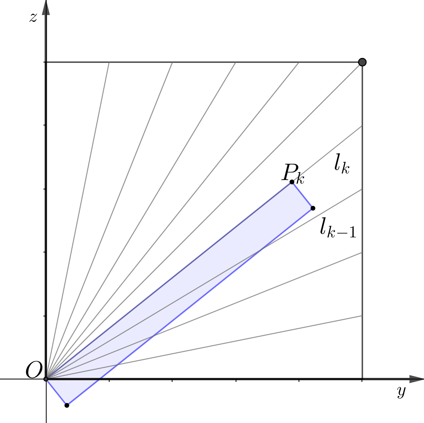
For satisfying and , we have
Now,
Next, we take such that . For each , we consider the rectangle containing of dimensions with one of its shorter side touching the circle centered at origin and of radius and the longer side is parallel to the line and lying below the line . We note that the equation of lines for longer sides of the rectangle are and and the equation of lines for shorter sides are and Thus,
Therefore we have,
∎
10. Further discussions
In this section we initiate a discussion about connections of bilinear Kakeya maximal function with other type of maximal functions in the bilinear setting. The aim of this discussion is to indicate some further questions that need to be investigated.
Let denote the set of vectors in and given a collection of rectangles we use the notation to denote the collection of those rectangles in which have their longest side parallel to some . If not stated otherwise, the elements of will be unit vectors.
For the linear case, when is the collection of rectangles with longest side parallel to one of the vectors in and , the operator defined in (2.1) satisfies the bound,
The above inequality was shown to hold by Strömberg [27] for the uniformly distributed set of directions and for arbitrary set of directions, this was resolved by Katz [12]. Moreover, for the lacunary set of directions, was shown to be weak type by Córdoba and Fefferman [8], and it was proved to be bounded in in [22] using Fourier transform methods.
We define the directional bilinear maximal operator by
Here we would like to refer the interested reader to Strömberg [27], Córdoba and Fefferman [8], Katz [12], Nagel, Stein and Wainger [22] for some of the important results for the linear counterpart
Another important class of maximal functions in the bilinear theory, as studied by Lacey [16], is defined as
| (10.1) |
where . Observe that if , then estimates for can be easily deduced from that of the Hardy-Littlewood maximal function. In the remaining cases, Lacey [16] proved that for , the operator maps into for and . It is well-known that the maximal function is intimately connected with the bilinear Hilbert transforms.
Next, we observe that with the use of Lebesgue differentiation theorem, one can deduce that
where This relation naturally gives rise to questions and probable methods to address issues related to boundedness of both the maximal functions.
Remark 10.1.
We have few observations in order highlighting the dependence on of the operator when is near the diagonal. It is evident from the example given in Proposition 9.1 that the operator fails to be bounded from into . A modification in example as given below, allows us to show that the where grows logarithmically in . This shows that is not uniformly bounded in the neighbourhood of .
Observation: Let where is a small constant, then The following example proves this assertion.
Example 10.2.
For consider and . Note that
For , consider the rectangle containing the point with dimension and having its longest side in the direction of with and as two vertices on the longer side. Note that the long sides of are given by and Consider
Since is large and is a fixed small constant, then for we see that
Thus, we get that
This implies that
∎
Acknowledgement
Ankit Bhojak and Saurabh Shrivastava acknowledge the financial support from Science and Engineering Research Board, Department of Science and Technology, Govt. of India, under the scheme Core Research Grant, file no. CRG/2021/000230. Surjeet Singh Choudhary is supported by CSIR(NET), file no.09/1020(0182)/2019- EMR-I for his Ph.D. fellowship.
References
- [1] Bernicot, F., Grafakos, L., Song, L., and Yan, L. The bilinear Bochner–Riesz problem. J. Anal. Math. 127 (2015), 179-217.
- [2] Bernicot, F., and Germain, P. Boundedness of bilinear multipliers whose symbols have a narrow support. J. Anal. Math. 119 (2013), 166-212.
- [3] Choudhary, S.S., Jotsaroop K., Shrivastava, S., and Shuin, K. Blinear Bochner-Riesz square function and applications. arXiv:2107.00840v3.
- [4] Choudhary, S.S. and Shrivastava, S. On the blinear Bochner-Riesz problem at critical index. J. Geom. Anal. 33 (2023), no. 2, Paper No. 58, 33 pp.
- [5] Cladek, L. Multiplier transformations associated with convex domains in . J. Geom. Anal. 26 (2016), no. 4, 3129-3175.
- [6] Cladek, L. On the square function associated with generalized Bochner-Riesz means. Indiana Univ. Math. J. 66 (2017), no. 6, 2205-2238.
- [7] Córdoba, A. The Kakeya maximal function and the spherical summation multipliers. Amer. J. Math. 99 (1977), no. 1, 1-22.
- [8] Córdoba, A., and Fefferman, R. On differentiation of integrals. Proc. Nat. Acad. Sci. U.S.A. 74 (1977), no. 6, 2211-2213.
- [9] Demeter, C., and Gautam, S. Z. Bilinear Fourier restriction theorems. J. Fourier Anal. Appl. 18 (2012), no. 6, 1265-1290.
- [10] Grafakos, L. Modern Fourier analysis. Third edition. Graduate Texts in Mathematics, 250. Springer, New York, (2014).
- [11] Grafakos, L., and Li, X. The disc as a bilinear multiplier. Amer. J. Math. 128 (2006), no. 1, 91-119.
- [12] Katz, N. Maximal operators over arbitrary sets of directions. Duke Math. J. 97 (1999), no. 1, 67–79.
- [13] Jeong, E., and Lee, S. Maximal estimates for the bilinear spherical averages and the bilinear Bochner-Riesz operators. J. Funct. Anal. 279 (2020), no. 7, 108629, 29 pp.
- [14] Jeong, E., Lee, S., and Vargas, A. Improved bound for the bilinear Bochner-Riesz operator. Math. Ann. 372 (2018), no. 1-2, 581-609.
- [15] Jotsaroop, K., and Shrivastava, S. Maximal estimates for bilinear Bochner-Riesz means. Adv. Math. 395 (2022), Paper No. 108100, 38 pp.
- [16] Lacey, M. T. The bilinear maximal functions map into for . Ann. of Math. (2) 151 (2000), no. 1, 35-57.
- [17] Lacey, M. T., and Thiele, C. estimates on the bilinear Hilbert transform for . Ann. of Math. (2) 146 (1997), no. 3, 693-724.
- [18] Lacey, M. T., and Thiele, C. On Calderón’s conjecture. Ann. of Math. (2) 149 (1999), no. 2, 475-496.
- [19] Liu, H., and Wang, M. Boundedness of the bilinear Bochner-Riesz means in the non-Banach triangle case. Proc. Amer. Math. Soc. 148 (2020), no. 3, 1121-1130.
- [20] Mohanty, P., and Shrivastava, S. Vector valued bilinear maximal operator and method of rotations. J. Math. Anal. Appl. 382 (2011), no. 1, 334–338.
- [21] Muscalu, C. L(p) Estimates for Multilinear Operators Given by Singular Symbols. Thesis (Ph.D.)–Brown University. 2000. 145 pp. ISBN: 978-0599-93764-2 ProQuest LLC.
- [22] Nagel, A., Stein, E. M., and Wainger, S. Differentiation in lacunary directions. Proc. Nat. Acad. Sci. U.S.A. 75 (1978), no. 3, 1060-1062.
- [23] Rubio de Francia, J.L. A Littlewood-Paley inequality for arbitrary intervals. Rev. Mat. Iberoamericana 1 (1985), no. 2, 1-14.
- [24] Saari, O., and Thiele, C. Paraproducts for bilinear multipliers associated with convex sets. Math. Ann. 385, 2013–2036 (2023).
- [25] Seeger, A., and Ziesler, S. Riesz means associated with convex domains in the plane. Math. Z. 236 (2001), no. 4, 643-676.
- [26] Stein, E. M. Harmonic analysis: real-variable methods, orthogonality, and oscillatory integrals. with the assistance of Timothy S. Murphy. Princeton Mathematical Series, 43. Monographs in Harmonic Analysis, III. Princeton University Press, Princeton, NJ, 1993. xiv+695 pp.
- [27] Strömberg, J. O. Maximal functions associated to rectangles with uniformly distributed directions. Ann. of Math. (2) 107 (1978), no. 2, 399-402.
- [28] Tanaka, H. An elementary proof of an estimate for the Kakeya maximal operator on functions of product type. Tohoku Math. J. (2) 48 (1996), no. 3, 429-435.
- [29] Trebels, W. Some Fourier multiplier criteria and the spherical Bochner-Riesz kernel. Rev. Roumaine Math. Pures Appl. 20 (1975), no. 10, 1173-1185.