Multi-object Video Generation
from
Single Frame Layouts
Abstract
In this paper, we study video synthesis with emphasis on simplifying the generation conditions. Most existing video synthesis models or datasets are designed to address complex motions of a single object, lacking the ability of comprehensively understanding the spatio-temporal relationships among multiple objects. Besides, current methods are usually conditioned on intricate annotations (e.g. video segmentations) to generate new videos, being fundamentally less practical. These motivate us to generate multi-object videos conditioning exclusively on object layouts from a single frame. To solve above challenges and inspired by recent research on image generation from layouts, we have proposed a novel video generative framework capable of synthesizing global scenes with local objects, via implicit neural representations and layout motion self-inference. Our framework is a non-trivial adaptation from image generation methods, and is new to this field. In addition, our model has been evaluated on two widely-used video recognition benchmarks, demonstrating effectiveness compared to the baseline model.
Index Terms:
Video Synthesis, Multi-object Scene, Generative ModelingI Introduction
Recent developments on video generation have enabled us to synthesize motion-coherent videos, by building variants on the generative adversarial network (GAN) [1]. The popularities are usually gained on videos of a specific dynamic object (e.g. Tai-Chi-HD dataset [2]), or of a specific action domain (e.g. Kinetics-serious dataset [3]). However, real-life scenes mostly involve multiple distinct instances with multiplex locations with dynamics. Other than that, there is undoubtedly an increasing demand to make the generation more tractable with a relatively simple generation condition, as an evidence, one of the recent trends of image generation is to condition only on scene graphs [4]. To achieve the above two goals, we seek to generate multi-object videos conditioned exclusively on layouts in a single frame.
A trivial method is to use current layout-to-image models [5, 6] in a frame-by-frame manner, omitting significant amount of temporal information implicit in the training video, and perhaps requiring supervisions in every frame. As a rather advanced solution, we may encode the dynamics of object locations together with static object features and other semantics to avoid over supervision, while making the inference of multi-object motions more straightforward and flexible. See Fig.1 for a brief illustration.

We build up our model — a Multiple Object Video Generative Adversarial Network (MOVGAN) — based on implicit neural representations (INR) [7], for it offering powerful differentiable continuous signal representations, which in our case, is able to map the generated sequential layout coordinates to high-level features. To achieve the multiple instances motion inference, similar to layout-to-image tasks [8], both the discriminator and the generator of MOVGAN are incorporated with spatial transform neural (STN) [9] layers to embed a relatively larger amount of object locations. From model architecture perspective, perhaps the most related works are the recent INR-based GAN [10, 7] for video generation, since our model can be seen as a generalization from theirs, by embedding instance-level layouts into both the discriminator and generator.
Our contributions can be summarized as follows:
- •
We are the very first kind to study video synthesis based exclusively on layouts from a single frame, and this is useful in some certain cases.
- •
Under our setup, the dynamics of multi-object locations are self-inferred from a single frame, and are dealt separately from other semantics before amalgamation, providing flexibility in modeling object motions.
- •
II Related Work
Layout-to-image Generation.
Since a video can be naively treated as an image sequence, image generation methods [1, 15] have an unavoidable enlightenment on video generation tasks. One of the most noticeable goal of image generation is to attain better controllability even for fine details [16, 17, 18]. Such researches usually resort to auxiliary supervisions such as instance-level segmentation masks [19], bounding boxes [20, 21], textual descriptions [22] and image layouts [5, 6]. Among them, coarse layouts (includes bounding boxes and categories) were recognized as perhaps the most flexible and controllable mechanism. Motivated by this, we seek to generalize from layout-to-image generation to layout-to-video generation.
Video Synthesis.
Most video synthesis prior works were task-driven, and can be broadly categorized with respect to the object quantity in the scene — single or multiple. Single object tasks favour strongly restricted conditions (e.g. a supplementary source image or video from the same domain) as their semantic source, for example, the talking head generation [23, 24], image animation [2, 25] and occlusion removal [26]. On the other hand, multi-object tasks are more challenging, and commonly apply weakly restricted conditions, such as action labels and language descriptions [10, 27]. Nonetheless, to better control the synthetic video, recent multi-object tasks intend to bring in strong restrictions such as segmentations [28] and scene graphs [29], to perform under a video-to-video paradigm . Our method, instead, detaches multiple layout motions from the overall framework and enjoys freedom for modeling object motions in a simple layout-to-video paradigm.


III Methodology
In this section, we will elaborate our generative framework by first introducing some necessary notations, then describing the major components, and finally presenting the overall learning formula. Our model MOVGAN is built upon DiGAN [10] with layout specifics, where both the generator and discriminator are designed to embody layout-encoding modules [8]. The overall generative backbone is a typical conditional sequential GAN [30], incorporating one latent video generator and a discriminator with two heads to respectively examine image and video authenticity.
Model Setup.
Mathematically, our goal is to approximate the real video distribution with a video model distribution .
Following the settings of [10], we assume a video is a sample from , i.e. . The video is 3-dimensional mapping from spatial coordinates and time of frame to the corresponding RGB signals: . Conditioning on a multi-layer perception (MLP) with parameter , the INR is denoted as . Given a video of size , we can decode the INR by computing the values of predefined coordinate grids (possibly equally-spaced). In this sense, the INR parameter is generated from the generator with latent variable (typically distributed as Gaussian): . The mapping is treated as a generator in GAN, being adversarially learned together with a discriminator .
Layout-to-video INR Generator.
We depict the complete pipeline of our generator in Fig. 2(a), as can be seen, it contains two streams — a global and a local pathways — respectively being designed for global scene and local objects generation.
In the global pathway (I), takes a random latent vector, the per-frame texture vector and the object layout coordinates , as inputs to generate global video canvas feature . Global function in (I) processes the labels of each and replicates them spatially to their locations. In fields where the bounding boxes are overlapped, the label embeddings are wrapped up, whereas the areas with no bounding boxes are filled with zero. Convolutional layers are then applied to each layout to obtain a high-level layout encoding, thereupon concatenated with to generate the image global feature .
The local pathway (II) controls the generation of local features by merely taking object identities as inputs. Each will be further transformed sequentially to locate at the corresponding layout location in the canvas through STN layers. The areas outside layout boxes will still remain zero. The two streams are then combined together to concatenate the global and local features, and , along the channel axis to be synthesized and up-scaled into the final resolution.
The dynamic synthetic module (V) generally follows the INR generation process. Denote the final implicit feature map as , we have , where ,, and are the weights and biases of the first layer in the dynamic synthetic module (V); , , are the frequencies of coordinates in video INR . Note that only the term is viewed as a continuous trajectory over time and is determined by parameters excluding , . In this sense, we can simply split the combination neural layers into two modules, and , so that manages the synthesis of static object/background and animates the outcome of . As the input of , is the latent vector that squeezes the layout coordinates and/or motions, namely, is defined as coordinates motion feature .
Visual and Motion Discriminator.
Our discriminator is formulated to recognize both the visual-cohesion and the motion-coherent of input videos. As displayed in Fig. 2(b), we follow the same spirit in building the generator , that two pathways in the discriminator are configured to extract global/local features.
The obtained global and local features are further concatenated together with the original video and fed into the downstream classifiers. The two classifiers, denoted by and , respectively identifies static and dynamic visual features. is a classical image discriminator that takes each frame of the video as input to differentiate its authenticity; is relatively complicated that distinguishes the triplet , where is the time gap between two frames and . Differing from , broadens the input channel from 3 to 7, where the 6th channel is implemented to represent two input video frames and the first channel is for . In addition, takes the extracted layout features (both global and local) of frames and as the input to finely identify the objects’ motion by locations.
Adversarial Learning.
The learning of our model follows directly from typical conditional GAN under the video generation setting. Considering the coarse layout with location and category , the goal of our model is to optimize the following minimax objective function:
| (1) | ||||
In (1), is the integrated generator function and . Therefore, can be expanded as
| (2) |
where stands for the neural function specified in the module (V). here is slightly different from by ignoring the layout , since the object layout/movement information is already embedded in axis motion modeling.
On the other hand, we split the discriminator function into and in the visual motion module (VI) (see Fig. 2(b)). Therefore, and share the layout information conveyed in discriminative pathways (III) and (IV), and we denote as a function to fuse layout labels with frame at time . In this sense, the discriminator function in (1) is defined as:
| (3) | ||||
Note that in this equation, we have specified both and labels. To avoid confusion, we may explain this with: during the adversarial learning of the discriminator, and are training layout inputs at time and , which serve to retain the dynamics between two consecutive frame layouts or object pixels, so that it is consistent with the ground-truth motion pattern.
IV Experiments
The main purpose of this section is to compare MOVGAN with a baseline model, and since there is nearly no algorithm available in our setting, our goal is not to establish state-of-the-art practical performance. Instead, these simulation studies serve to verify the effectiveness of our adjustable layout motion inference from four aspects: (1) the capability of generating multi-object videos; (2) the temporal consistency of the generated objects given specific layouts; (3) the visual quality and quantitative scores; (4) the flexibility in editing the generated video.
| VidVRD | ||||
| Model | FID | FVD | ||
| 64 | 128 | 64 | 128 | |
| TGAN-F | 66.23 | 87.92 | 665.16 | 1002.37 |
| Baseline DiGAN | 63.54 | 79.20 | 589.14 | 983.74 |
| TGAN-F+ISLA-Norm | 60.31 | 78.03 | 583.90 | 881.11 |
| DiGAN+ISLA-Norm | 59.02 | 68.91 | 579.11 | 898.62 |
| MOVGAN (ours) | 57.72 | 63.52 | 567.31 | 877.22 |
| VidVOR (20 max instance) | ||||
| T-GAN-F | 142.29 | 216.33 | 2445.33 | 3622.71 |
| TGAN-F+ISLA-Norm | 140.98 | 223.21 | 2536.87 | 3482.28 |
| Baseline DiGAN | 125.8 | 156.79 | 2138.81 | 2309.12 |
| DiGAN+ISLA-Norm | 114.92 | 134.82 | 2039.2 | 2156.79 |
| MOVGAN (ours) | 101.22 | 123.78 | 1781.43 | 2009.86 |
IV-A Datasets
We have adopted 2 datasets of progressively increased complexity — VidVRD [11] and VidVOR [12, 13]. These two benchmarks were originally created for complex scene video recognition, involving multiple complex scenes, such as indoor and outdoor interactive objects with different light conditions and various camera perspectives. Most
importantly, instance-level labels and bounding boxes of each frame are easily accessible. For all models, we consider a maximum instance number of 11 and 20 respectively for VidVRD and VidVOR; the maximum category number is set to be 36 and 80 respectively for VidVRD and VidVOR. Further details of these two datasets are listed in Appendix A.

IV-B Baselines and Experimental Settings
Our baseline model is an adaptation of DiGAN into our setting by conditioning only on multi-object labels (no layouts). The biggest difference between MOVGAN and the baseline has been shown in Section III, in local pathway (II) of generator , where identity embedding layers are introduced. Except this, the baseline model is maintained nearly identical to MOVGAN for equal comparison. In practice, those identity embedding layers are implemented based on styleGAN [31]: the number of linear neural layers of style encoding is set to be 4; the convolutional module is implemented using SkipNet [32] without batch normalization. For more practical reasons, the parameter accuracy of the discriminator is reduced to float16 (default is float32). Our batch size is 8 with 25,000 frames per epoch, the learning rate is .
IV-C Metrics
For evaluating per-frame image quality, we measure the Fréchet Inception Distance (FID) [33], whereas for measuring motion-coherency, we choose the Fréchet Video Distance (FVD) [34]. For a quick comparison, the inception network of FVD is a specially pretrained inflated 3D Convnet [35] for sequential data, for the purpose of estimating distributions over an entire video.
IV-D Quantitative Results
Compared with Baselines
We provide FID and FVD figures for videos of sizes 6464 and 128128 in Table I. Comparing with the baseline model DiGAN, we see a clear drop of MOVGAN on both scores. This indicates that layout information embedding indeed helps the model to attain better image quality and motion continuity. From table I, TGAN-F [36] is another video generation baseline. We have also attached a layout embedding approach proposed in [20], called ISLA-Norm. As can be seen that, our layout motion embedding works better than that of the ISLA-Norm in all records.
Discriminator Logits
A further evidence of the improvement is displayed through the discriminator logits curves in Fig. 4. In particular, the y axis values are calculated between real videos and fake videos : for MOVGAN is ; for Baseline is , where one-hot multi-label encoding has been implemented to infuse object identities . Error bars of each curve indicate ±1 standard deviation computed with respect to the batch mean. We observe that MOVGAN generally achieves lower discriminator logits, implying better approximations of the real video distribution.
IV-E Alation Study
Herein, we would like to provide an additional ablative performance evaluation of MOVGAN. The model variants to be measured include:
- •
Action label (DiGAN, green curve)
- •
Multiple-class-object label (+MCOL, yellow curve)
- •
Centralized crop (+CC, blue curve)
- •
Multiple-object layout (+MOL, purple curve)
- •
Multiple-object layout with object identification loss (equation (1), MOVGAN, red curve)
For a closer look, we have displayed some of the results in Figure 6, where we have used 5 curves of different colours to indicate the above mentioned variables. We observe that, by step-wisely applying each of the components to the baseline, FID and FVD gradually converge to lower values. In particular, we find object layouts (+MOL) are especially beneficial for FVD, which is indeed the case that layout information is crucial in video synthesis. Henceforth, we may safely conclude that each of the applied component in MOVGAN is effective in their own sense.
IV-F Intriguing Property
Visualizations and Video Manipulation.
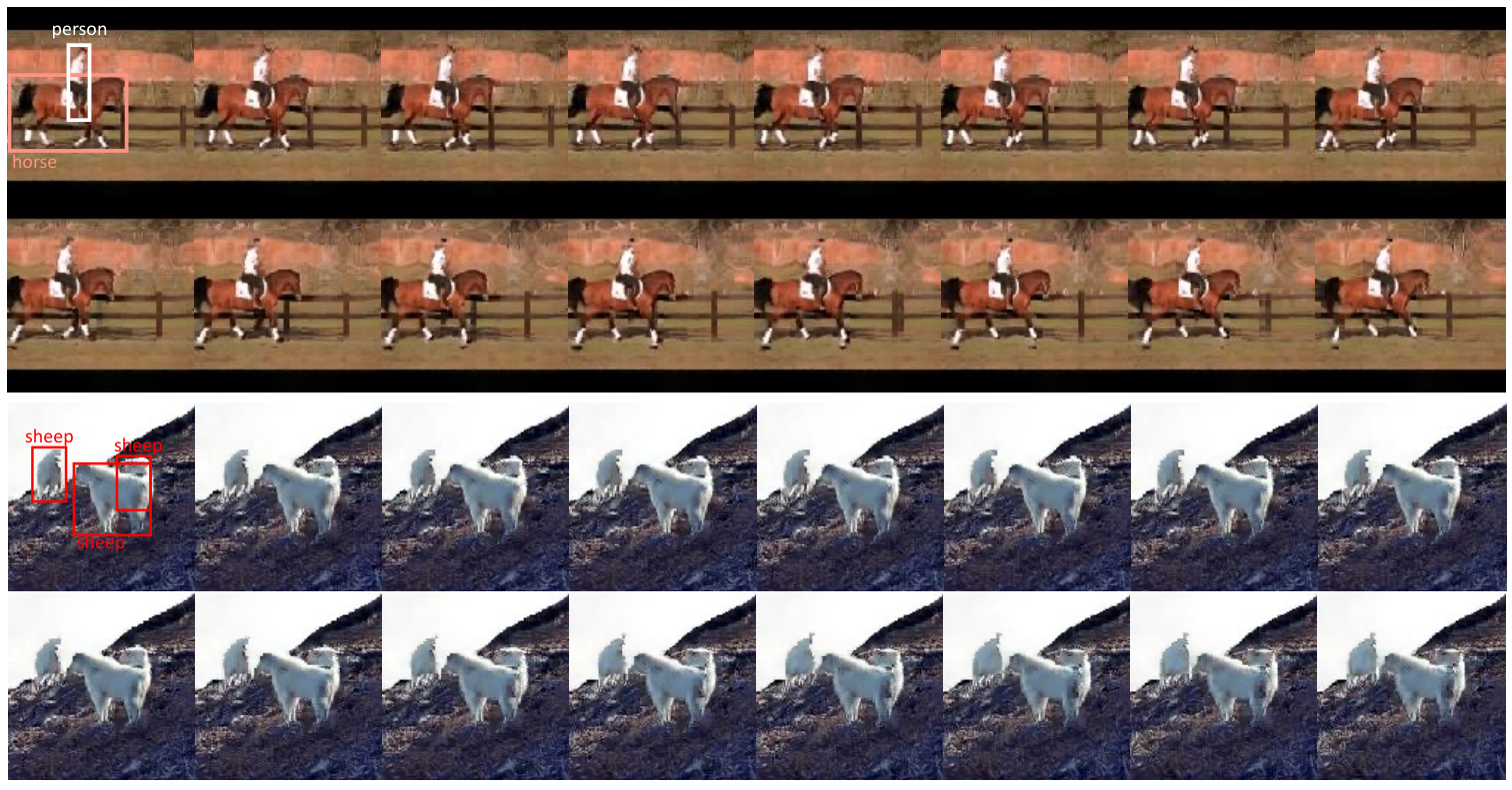
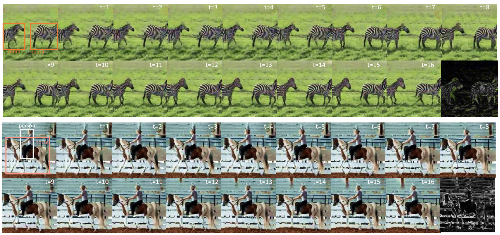
In Fig. 3, from the top row to the bottom row, we provide video editing examples of three types: ‘adding’ a ‘cow’, ‘removing’ a ‘person’ and ‘resizing’ two ‘horses’. These results have shown the ability of our model in easily operating on fine-level features. Moreover, in these 6 figures and results shown in Fig.5, from left to right, though being minuscule11
1
We suggest this is mainly due to the difficulty of the dataset, but since our model is specially designed for multi-objects, it is not our scope to revise our model to fit single object scenarios. However, it may be of interest to seek refined techniques in future works., object motions can be observed.
Resolution Augmentation.
We have also managed to furnish an augmentation trick to the current model to rise the resolution of the synthetic videos. Detailed techniques and results can be found in Appendix B.
V Conclusion
In this paper, we have proposed a new video synthesis framework based on implicit neural representation GAN models, allowing spatio-temporal inference in multiplex scenes. The notable feature of our model is to depend only on layout information from a single frame and self-inferring the dynamics, opening up the possibility for scenarios with limited supervisions. In future works, it may be of interest to address some of the remaining gaps, such as refining our model or composing complete new methods to achieve greater object movements and more logical interactions.
Acknowledgment
This work was supported in part by National Key R&D Program of China under Grant No. 2021ZD0111601, National Natural Science Foundation of China (NSFC) under Grant No. 61836012 and 62272494, Guangdong Basic and Applied Basic Research Foundation under Grant No. 2023A1515012845 and 2023A1515011374. Also, we want to appreciate Dr. Xu Cai from National University of Singapore for his contributions to this paper. The corresponding author of this paper is Hefeng Wu.
References
- [1] I. Goodfellow, J. Pouget-Abadie, M. Mirza, B. Xu, D. Warde-Farley, S. Ozair, A. Courville, and Y. Bengio, “Generative adversarial networks,” Communications of the ACM, vol. 63, no. 11, pp. 139–144, 2020.
- [2] A. Siarohin, S. Lathuilière, S. Tulyakov, E. Ricci, and N. Sebe, “First order motion model for image animation,” in NeurIPS, 2019.
- [3] J. Carreira, E. Noland, A. Banki-Horvath, C. Hillier, and A. Zisserman, “A short note about kinetics-600,” arXiv preprint arXiv:1808.01340, 2018.
- [4] R. Herzig, A. Bar, H. Xu, G. Chechik, T. Darrell, and A. Globerson, “Learning canonical representations for scene graph to image generation,” in ECCV, 2020.
- [5] J. Li, T. Xu, J. Zhang, A. Hertzmann, and J. Yang, “LayoutGAN: Generating graphic layouts with wireframe discriminator,” in ICLR, 2019. [Online]. Available: https://openreview.net/forum?id=HJxB5sRcFQ
- [6] B. Zhao, L. Meng, W. Yin, and L. Sigal, “Image generation from layout,” in CVPR, 2019, pp. 8584–8593.
- [7] I. Skorokhodov, S. Ignatyev, and M. Elhoseiny, “Adversarial generation of continuous images,” in CVPR, 2021, pp. 10 753–10 764.
- [8] T. Hinz, S. Heinrich, and S. Wermter, “Generating multiple objects at spatially distinct locations,” in ICLR, 2019. [Online]. Available: https://openreview.net/forum?id=H1edIiA9KQ
- [9] M. Jaderberg, K. Simonyan, A. Zisserman et al., “Spatial transformer networks,” Advances in neural information processing systems, vol. 28, 2015.
- [10] S. Yu, J. Tack, S. Mo, H. Kim, J. Kim, J.-W. Ha, and J. Shin, “Generating videos with dynamics-aware implicit generative adversarial networks,” in ICLR, 2022. [Online]. Available: https://openreview.net/forum?id=Czsdv-S4-w9
- [11] X. Shang, T. Ren, J. Guo, H. Zhang, and T.-S. Chua, “Video visual relation detection,” in ACM International Conference on Multimedia, Mountain View, CA USA, October 2017.
- [12] X. Shang, D. Di, J. Xiao, Y. Cao, X. Yang, and T.-S. Chua, “Annotating objects and relations in user-generated videos,” in Proceedings of the 2019 on International Conference on Multimedia Retrieval. ACM, 2019, pp. 279–287.
- [13] B. Thomee, D. A. Shamma, G. Friedland, B. Elizalde, K. Ni, D. Poland, D. Borth, and L.-J. Li, “Yfcc100m: The new data in multimedia research,” Communications of the ACM, vol. 59, no. 2, pp. 64–73, 2016.
- [14] A. Nagrani, J. S. Chung, and A. Zisserman, “Voxceleb: a large-scale speaker identification dataset,” in INTERSPEECH, 2017.
- [15] D. P. Kingma, M. Welling et al., “An introduction to variational autoencoders,” Foundations and Trends® in Machine Learning, vol. 12, no. 4, pp. 307–392, 2019.
- [16] P. Sangkloy, J. Lu, C. Fang, F. Yu, and J. Hays, “Scribbler: Controlling deep image synthesis with sketch and color,” in Proceedings of the IEEE conference on computer vision and pattern recognition, 2017, pp. 5400–5409.
- [17] K. K. Singh, U. Ojha, and Y. J. Lee, “Finegan: Unsupervised hierarchical disentanglement for fine-grained object generation and discovery,” in Proceedings of the IEEE/CVF conference on computer vision and pattern recognition, 2019, pp. 6490–6499.
- [18] Y. Men, Y. Mao, Y. Jiang, W.-Y. Ma, and Z. Lian, “Controllable person image synthesis with attribute-decomposed gan,” in Proceedings of the IEEE/CVF conference on computer vision and pattern recognition, 2020, pp. 5084–5093.
- [19] X. Liu, G. Yin, J. Shao, X. Wang et al., “Learning to predict layout-to-image conditional convolutions for semantic image synthesis,” Advances in Neural Information Processing Systems, vol. 32, 2019.
- [20] W. Sun and T. Wu, “Image synthesis from reconfigurable layout and style,” in Proceedings of the IEEE/CVF International Conference on Computer Vision, 2019, pp. 10 531–10 540.
- [21] T. Sylvain, P. Zhang, Y. Bengio, R. D. Hjelm, and S. Sharma, “Object-centric image generation from layouts,” in Proceedings of the AAAI Conference on Artificial Intelligence, vol. 35, no. 3, 2021, pp. 2647–2655.
- [22] A. Ramesh, M. Pavlov, G. Goh, S. Gray, C. Voss, A. Radford, M. Chen, and I. Sutskever, “Zero-shot text-to-image generation,” in International Conference on Machine Learning. PMLR, 2021, pp. 8821–8831.
- [23] E. Zakharov, A. Shysheya, E. Burkov, and V. Lempitsky, “Few-shot adversarial learning of realistic neural talking head models,” in Proceedings of the IEEE/CVF international conference on computer vision, 2019, pp. 9459–9468.
- [24] L. Chen, G. Cui, C. Liu, Z. Li, Z. Kou, Y. Xu, and C. Xu, “Talking-head generation with rhythmic head motion,” in European Conference on Computer Vision. Springer, 2020, pp. 35–51.
- [25] K. Sarkar, D. Mehta, W. Xu, V. Golyanik, and C. Theobalt, “Neural re-rendering of humans from a single image,” in European Conference on Computer Vision. Springer, 2020, pp. 596–613.
- [26] F. Pizzati, P. Cerri, and R. d. Charette, “Model-based occlusion disentanglement for image-to-image translation,” in European conference on computer vision. Springer, 2020, pp. 447–463.
- [27] S. Ge, T. Hayes, H. Yang, X. Yin, G. Pang, D. Jacobs, J.-B. Huang, and D. Parikh, “Long video generation with time-agnostic vqgan and time-sensitive transformer,” arXiv preprint arXiv:2204.03638, 2022.
- [28] A. Mallya, T.-C. Wang, K. Sapra, and M.-Y. Liu, “World-consistent video-to-video synthesis,” in European Conference on Computer Vision. Springer, 2020, pp. 359–378.
- [29] Y. Cong, J. Yi, B. Rosenhahn, and M. Y. Yang, “Ssgvs: Semantic scene graph-to-video synthesis,” ArXiv, vol. abs/2211.06119, 2022.
- [30] Y. Wang, P. Bilinski, F. Bremond, and A. Dantcheva, “Imaginator: Conditional spatio-temporal gan for video generation,” in Proceedings of the IEEE/CVF Winter Conference on Applications of Computer Vision, 2020, pp. 1160–1169.
- [31] T. Karras, S. Laine, M. Aittala, J. Hellsten, J. Lehtinen, and T. Aila, “Analyzing and improving the image quality of stylegan,” in Proceedings of the IEEE/CVF conference on computer vision and pattern recognition, 2020, pp. 8110–8119.
- [32] X. Wang, F. Yu, Z.-Y. Dou, T. Darrell, and J. E. Gonzalez, “Skipnet: Learning dynamic routing in convolutional networks,” in Proceedings of the European Conference on Computer Vision (ECCV), 2018, pp. 409–424.
- [33] M. Heusel, H. Ramsauer, T. Unterthiner, B. Nessler, and S. Hochreiter, “Gans trained by a two time-scale update rule converge to a local nash equilibrium,” in Advances in Neural Information Processing Systems, 2017, pp. 6629–6640.
- [34] T. Unterthiner, S. van Steenkiste, K. Kurach, R. Marinier, M. Michalski, and S. Gelly, “Towards accurate generative models of video: A new metric & challenges,” arXiv preprint arXiv:1812.01717, 2018.
- [35] J. Carreira and A. Zisserman, “Quo vadis, action recognition? a new model and the kinetics dataset,” in proceedings of the IEEE Conference on Computer Vision and Pattern Recognition, 2017, pp. 6299–6308.
- [36] M. Saito, S. Saito, M. Koyama, and S. Kobayashi, “Train sparsely, generate densely: Memory-efficient unsupervised training of high-resolution temporal gan,” International Journal of Computer Vision, vol. 128, no. 10-11, pp. 2586–2606, 2020.
- [37] R. Yang, P. Srivastava, and S. Mandt, “Diffusion probabilistic modeling for video generation,” arXiv preprint arXiv:2203.09481, 2022.
Appendix A Data Refinement
Statistics. Here we present the detailed statistics of the considered two datasets. Since these data are now made to serve video synthesis, we seek to optimize the datasets to fit with our experimental setting:
- •
We have taken out possible invalid frames (e.g. those without any object of interest), to avoid data contamination.
- •
We have made the data to be balanced with respect to different object quantities, since majority of the videos only contain two objects.
- •
We have filtered those video clips with their instance amount exceeding the maximum value we set (mentioned in Section IV).
Eventually, the statistics of the refined datasets can be found in Table II.
| Dataset | #Video | #Category | #Valid Frame | #Max Instance |
|---|---|---|---|---|
| VidVRD | 1,000 | 35 | 46,930 | 11 |
| VidVOR | 10,000 | 80 | 6,834,925 | 26 |
| VidVRD | ||||
| Model | FID | FVD | ||
| 128 | 256 | 128 | 256 | |
| MOVGAN (ours) | 63.52 | 72.35 | 877.22 | 983.74 |
| MOVGAN+ Diff (ours) | 54.67 | 58.26 | 890.20 | 991.56 |
| VidVOR (20 max instance) | ||||
| MOVGAN (ours) | 123.78 | 153.25 | 1781.43 | 2223.32 |
| MOVGAN+ Diff (ours) | 112.12 | 124.78 | 2002.91 | 2329.36 |
Appendix B Additional Experimental Results
B-A Resolution Augmentation
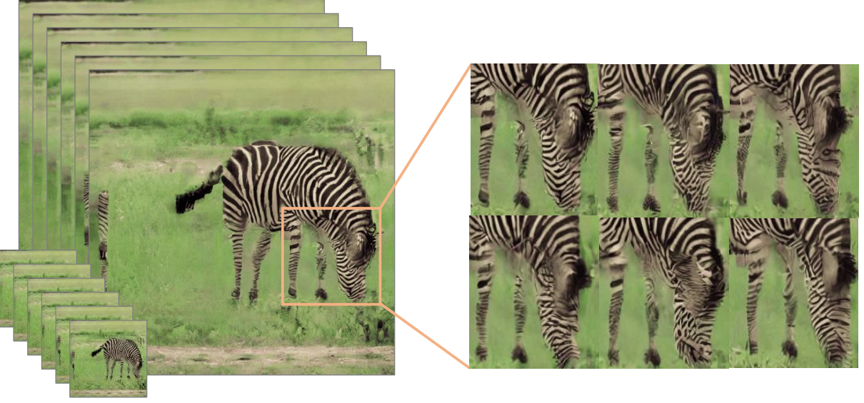

We provide synthetic results in higher resolutions using an augmentation trick, by applying a super resolution algorithm to each synthetic frame. The algorithm we use is the most recent stable diffusion model [37]. From Fig.7, we see little visual difference between the augmented synthetic and training sample, which is also verified through FID scores in Table III. However, at the same time, the FVD score becomes worse, and this might be the reason that some temporal information are missing during augmentation. Regarding this, it may require more advanced techniques to compensate object dynamics.
B-B Further Synthetic Videos