Weighted high dimensional data reduction of finite Element Features - An Application on High Pressure of an Abdominal Aortic Aneurysm
Abstract
In this work we propose a low rank approximation of high fidelity finite element simulations by utilizing weights corresponding to areas of high stress levels for an abdominal aortic aneurysm, i.e. a deformed blood vessel. We focus on the van Mises stress, which corresponds to the rupture risk of the aorta. This is modeled as a Gaussian Markov random field and we define our approximation as a basis of vectors that solve a series of optimization problems. Each of these problems describes the minimization of an expected weighted quadratic loss. The weights, which encapsulate the importance of each grid point of the finite elements, can be chosen freely - either data driven or by incorporating domain knowledge. Along with a more general discussion of mathematical properties we provide an effective numerical heuristic to compute the basis under general conditions. We explicitly explore two such bases on the surface of a high fidelity finite element grid and show their efficiency for compression. We further utilize the approach to predict the van Mises stress in areas of interest using low and high fidelity simulations. Due to the high dimension of the data we have to take extra care to keep the problem numerically feasible. This is also a major concern of this work.
Keywords Dimension Reduction Weights Computer Experiments Multifidelity Simulations Gaussian Markov Random Fields
1 Introduction
The starting point for the method which we develop in this work is a real world application whose nature is tightly connected to the concrete implementation. To be specific, we deal with data from a computationally expensive high fidelity computer simulation that returns the deformations and stresses of an abdominal aortic aneurysm (AAA) in response to blood pressure, see Biehler et al. 2014. This simulation is complex, yet deterministic and returns the vector , with denoting the outcome at location , where is a three-dimensional finite element grid. The outcome quantity is thereby the magnitude of the van Mises stress, which is a mechanical quantity that summarizes the tensor-valued stress at each grid point into one number. The simulation depends on a (tuning) parameter vector of wall parameters and we may therefore denote the outcome of the simulation as .

The outcome of a single simulation is shown as part of Figure 1 (first and third image). These finite element simulations can be used to assess the rapture risk of the blood vessel and to guide medical treatment in a real word scenario.
Because the high fidelity simulation is computationally expensive a two step approach has been proposed in Striegel et al. 2022 (see also Biehler et al. 2016) that uses adjusted low fidelity simulations on a simplified grid as a surrogate for the high fidelity computations. The low fidelity simulation can also be seen as part of Figure 1 (second and fourth image). We denote the low fidelity simulation with . While it can be useful to relate the entire low fidelity simulation to its high fidelity counterpart , as done in Striegel et al. 2022, it is omitted that one is mostly interested in high stress levels, as those indicate the risk of an aortic rupture, leading to internal bleeding, which, if not treated immediately, results in the death of the patient. In other words one aims not to predict the entire high fidelity outcomes but only high stress areas based on a low fidelity simulation . This is the goal of the following paper. To do so we pursue a weighted dimension reduction of through an optimally chosen basis, where the weights account for relevancy of each grid point on the high fidelity mesh with the focus on high stress and hence high risk of rupture. The basis is computed in an iterative way, where each basis vector solves an optimization problem based on the weighted expected quadratic compression error. While the unweighted problem is solved by simple eigenvectors, the addition of weights makes a new numerical solution necessary. As each basis vector has the dimension of the high fidelity grid, i.e. multiple thousand, the optimization is tedious and the numerical solution, which is highly optimized to our problem at hand, is a major contribution of this paper. However, the theoretical derivations given in the paper are applicable to any high dimensional Gaussian random field and even more broadly to any field with a given covariance structure.
Conceptually related work to our basis computation can be found in Gabriel and Zamir 1979, who present the approximation of a matrix with additional weights using a weighted least square loss. Tamuz et al. 2005 uses this approach to develop an effective algorithm to filter out systematic effects in light curves. Similarly to both papers, our work can be seen as a generalization of principal component analysis and uses numerical optimization instead of closed form solutions. Our methodology does assume a Gaussian random field and not a matrix as starting point and also our loss function incorporates the elementwise error for every component of the vector - not the cumulative error for all matrix elements. In this line, we consider our work as a straight forward extension to (general) eigenvalue decomposition and similar methods as presented in Ghojogh et al. 2019 and similarly it allows for dual formulations - though not as a matrix but as a more involved tensor decomposition. Taking the view of popular fields like computer vision and machine learning, the basis computation can be seen as the extraction of features from the grid with respect to a certain loss function. See Zebari et al. 2020 for a comprehensive survey or Soltanpour et al. 2017 for the more related usecase of feature extraction from 3D face images. In contrast to most methods applied in these fields however our work is designed to deal with very small sample sizes in the order of hundreds and even less, where machine learning typically is not applicable.
The remainder of this work is structured as follows: First, we will justify our modeling approach by discussing the nature of the data at hand. In the third part we will derive our data driven weights model which will deliver additional information for the weighted basis approach discussed in the fourth section. Here we define relevant problems for our basis vectors and provide ideas for an efficient solution along with exemplary basis vectors for our application at hand and an evaluation of their quality. We also touch the numerics behind the basis computation. Finally, in the fifth section, we evaluate the use of the weighted basis vectors for an exemplary application, the prediction of high fidelity stress values from low fidelity counterparts. The paper finishes with a brief discussion.
2 Review of the data
We define with the -th high fidelity simulation run with input parameter and accordingly with the matching low fidelity counterpart. The high fidelity outcome is of dimension and the dimension of the low fidelity counterpart is . Note that the computation of a single high fidelity outcome takes approximately CPU seconds (around hours), whereas the computation of a low fidelity simulation takes a mere CPU seconds (around minutes). This readily shows the value of a model that enables high fidelity predictions from low fidelity outcomes. The ultimate goal of the developed methodology is therefore to work based on small samples with only a limited amount of high and low fidelity simulations available. To be specific, we will only use few cases for the training and define the training set as , with . The data at hand trace from a larger experiment and we utilize the remaining data, which consists of observations for evaluating the performance of our approach. We denote the test set with .
As outlined in the introduction we are interested in high (van Mises) stress values. In what follows we will exemplary look at the top and values. In order to analyze the location where these values occur we plot the simple high stress frequency, i.e. the number of samples in the test set for which a high stress value is taken at a certain point, normalized by the number of simulations:
| (1) |
for a given quantile and a point . The results for both percentiles of interest are shown in Figure 2:

We can see that in both cases the values are spatially clustered on the grid. In particular there are no isolated grid points. While in the case of the top stress values only the front part of the geometry is of interest, for the top there are additional smaller stress centers at the back. The fact that the area at the crook has significantly lower stress may be surprising at first glance, but is in fact a direct consequence of the thrombus, i.e. a layer of coagulated blood that strengthens this part of the vessel.
Figure 3 gives the average number of points on the mesh above the quantile when increasing the sample size. We see that high values of van Mises stress tend to occur in similar regions and the number of relevant points on the mesh seems to be bounded when increasing the sample size. This shows that the spatial variance of the high stress areas is low and we can expect to reliably predict which parts of the grid are relevant for high stress.
Overall, as shown in Figure 2, we are dealing with locally clustered areas, i.e. some grid points are of higher interest than others. This is what we aim to take into account when applying dimension reduction tools. In fact, a simple eigenvector decomposition of the grid is less suitable to effectively compress the relevant information. The central contribution of this paper is therefore to construct a suitable basis for dimension reduction which will incorporate additional weights to deliver local features occurring in the data at hand.
3 Modeling of the weights
The first step is the construction of an appropriate weight vector. These weights should mirror the importance of each grid point and should be chosen data driven or, alternatively, by expert knowledge. In the following we take a data driven approach. The derivations are given for a general quantile .
There are multiple facts that we want to account for when estimating the relevancy of a specific point on the grid. Firstly, the points where high stress values occur in the training set are most important. Secondly, points in the local neighborhood of high stress values are informative as well. Finally, as we can see in the training set and as shown in Figure 3, high stresses do overlap between different samples and only vary slightly along the borders. Hence, these points of the mesh are of primary interest.
Given the already high amount of information in the training data and the spatial structure of the data we will use a smoothed version of the high stress frequencies as weight vector . We propose standard kernel smoothing with Gaussian kernels
| (2) |
Here defines the shortest path in edges between two points on the high fidelity grid. The smooth weights are then defined as
| (3) |
with defined as in (1). We can summarize this equation in a vector matrix form with . Here is the smoothing matrix containing the smoothing weights. Further we can select the bandwidth parameter with standard generalized cross validation (see Golub et al. 1979, Li 1986). We omit the plotting of the resulting weight vectors as there is a slight difference to Figure 2.
4 Finite Element features using additional weights
4.1 Basis Definition
Before we outline a general solution and look at some exemplary vectors, we define the weight based basis vectors for the high fidelity grid as a series of optimization problems. For this part we assume the existence of a weight vector with and . We assume further that the high fidelity output follows a Gaussian Markov Random Field (GMRF) assumption, i.e. . The mean vector is of secondary interest and for the covariance matrix we assume a GMRF precision matrix, , built from the finite elements structure. has zero entries except for
Here defines the neighborhood of point on the grid and we refer to Rue and Held 2005 for details. The goal is the approximation of with an orthonormal basis consisting of vectors , i.e. , with and . This basis depends on the weights and - as shown in the previous part - the corresponding stress quantile, i.e. .
4.1.1 First vector
We will compute the basis iteratively and start with a basis of length one consisting of the single vector . If we use this basis for a straight forward compression of it holds
| (4) | ||||
| (5) |
Using this distribution we define the following squared risk function, which summarizes the componentwise expected squared error
| (6) |
We choose the basis vector to minimize the expected L loss (6) and it therefore solves the optimization problem
| (7) |
One can easily show that this problem is equivalent to an eigenvector problem, i.e. the vector that solves this optimization problem is the eigenvector corresponding to the largest eigenvalue of .
Instead of Formula (6) we now incorporate the weight vector constructed above leading to a risk function with weighted componentwise compression errors:
| (8) |
with . The optimal basis then solves the optimization problem:
| (9) |
This problem is not equivalent to simple eigenvalue computation and we have to resort to numerical optimization algorithms. For the actual numeric computation it is preferable to use a slightly different version of the objective risk function, which we get from (8) by plugging in and simplifying:
| (10) |
This leads to the gradient and the Hessian matrix
| (11) | ||||
| (12) | ||||
4.1.2 From p to (p+1)
Given the basis vectors we then derive the basis vector as the vector that optimally compresses the remainder and is orthogonal to the previous basis vectors, i.e.
| (13) | ||||
Then it holds
| (14) | ||||
with . Analogously to above we can define a risk function which summarizes the weighted componentwise compression errors of the remainder
| (15) |
Given the first vectors of the basis the next vector of the basis is then given by an optimization problem with a different objective function:
| (16) |
If all weights are the same the optimal vector will be the -th eigenvector of . A simplified version of the risk function, the gradient and the Hessian can be computed similarly to (10), (11) and (12). We refer to the supplied code for further details.
4.1.3 Beyond the Gaussian
Strictly speaking, the derivations in section 4.1 only need the covariance matrix . The Gaussian distribution is not needed as all expectations in (6) can be expressed as linear combinations of variances and covariances of . This opens up the space for possible applications to any multivariate distribution where the covariance matrix is known and numerically treatable. In fact, we do not need a distribution at all and can just plug in an empirical estimate for .
4.2 Heuristic Solution
Solving the problems defined in (9) and (16) is nontrivial and needs some additional attention. First the series of optimization problems that lead to the basis are not convex. This is also true for the unconstrained case as well as the unweighted. Without going into details and depending on the nature of and the number of local minima is generally in the order of . These correspond to only bases of different compression quality due to the inherent symmetry of the problem, i.e. . This means that are in general a high number of possible local minima that render a brute force numerical optimization approach problematic. Standard approaches using a Lagrange multiplicator that iterate over different points on the surface of the unit cube are - depending on the choice of the starting point - much more likely to end up in a local minimum of the risk function than finding the global one. The deeper reason is the fact that the unconstrained objective function is after all a distorted version of the standard eigenvalue problem, i.e. the potential basis vectors are distributed around the origin, with at most one in each direction. The only point that gives us free access to all of them - the origin itself - however is not part of the available set of vectors. A possible solution is therefore to drop the normalization condition and start numerical optimization at zero - simply following the steepest descent. As the gradient itself vanishes at zero we will instead resort to the smallest eigenvector of the Hessian (12), i.e. use a Taylor approximation of rank two at zero. To get a basis vector we will finally normalize the resulting vector to one. Summing things up, this leaves us with the following heuristic for the first basis vector:
We take a similar approach for the following optimization problems in (16) and end up with the same algorithm but based on a different variance matrix and including an additional step to make sure the resulting vector is orthogonal to the previously computed ones. This algorithm is heuristic but provides - as we show in the following - good results in practice. Note also that the broader ideas behind this approach have been employed multiple times in the literature, see for example Ma et al. 2019.
Finally, want to stress that analogously to the unweighted case, which is equivalent to an eigenvector problem, our weighted basis has a connection to tensor decomposition. We have moved this mathematical reformulation to the Supplementary Material.
4.3 Numerical details
There are a number of minor numerical concerns that have to be addressed in order to make the problem solvable, which we have moved to the Appendix. Our heuristic itself has two steps: In order to compute the direction of the steepest descent for the starting point, as outlined in 4.2 we use the RSpectra (Xuan 2016) library. This allows for the computation of the most negative eigenvector of a matrix which is only specified by a function defining its product with an arbitrary vector and makes it as a result possible to compute the starting point without knowing the full Hessian.
Given this starting point each of these problems then requires its own optimization routine. There are a variety of solvers available for the problem at hand, which is as we have shown in 4.2 nonlinear and non-convex. We resort to the L-BFGS routine which is a standard Quasi-Newton algorithm if the gradient is available in a closed from but the Hessian isn’t. We refer to Nocedal and Wright 2006 for a general overview of numerical optimization. It would also be possible to use a classical Newton routine. We plug in the weight vectors computed in Section 3 into our framework and compute basis vectors for each stress quantile. The overall computation time per vector for both weight vectors is shown in Figure 4.
We can see that the computation time increases linearly with the number of the computed basis vectors. This follows directly from the problem formulation (16): Each vector depends on all the previously computed vectors which one by one add to the complexity of the objective function. There is no significant difference in cost when comparing both weight vectors, even though it might be slightly higher for the top stress values. The overall computation time of the weighted bases is significant - on average around hours or seconds for a basis of length . In combination with the diminishing effectiveness of additional basis vectors this steady increase in computation time make longer bases unattractive.
4.4 Discussion of the Basis vectors
The first four resulting vectors for the top stress values are shown in Figure 5. Basis vectors for the top values show a similar picture and are omitted.

As expected the basis vectors focus on the area in front where the weights are bigger and then vary the pattern of the weight vector as seen as a part of Figure 2. The remainder of the mesh grid is of little interest.
We are interested in the approximation quality the bases provide, i.e. its usability for compression, especially in comparison to ordinary unweighted GMRF bases. These latter bases simply take the leading eigenvectors of the GMRF covariance matrix and can be seen as a special case for a weight vector with equal weights. We look at the empirical error which we define as the simple mean squared compression error of the high stress values
| (17) |
Please notice that we restrict ourselves to the test set as the approximated outcomes depend on the weights derived from the training set. Further note that in practice we have to previously standardize our stress vectors by subtracting the sample mean in correspondence with our assumptions in 4.1. Results are shown in Figure 6.
The plot shows that the gain in compression quality decreases with each additional vector. Moreover, the top stress values are easier to compress with a weighted basis than the top . This is to be expected: Weighted bases get even more powerful for outcomes in a small area where the number of features can approach the number of grid points. For comparison we also show the compression error for the unweighted dimension reduction, i.e. with standard eigenvectors. Overall such comparison highlights that our approach indeed offers a great improvement with respect to the error. The approximation error for eigenvector bases is an order of magnitude larger than for their weighted counterparts. For bases of similar length we get errors which are up to three orders smaller. The extracted eigenvectors in the unweighted basis contain global features and the cutoff results in a significant loss of local information. A problem which we can solve with the introduction of weights.
We also plot the empirical compression errors on top of the geometry for the top stress values in Figure 7 to check for their spatial distribution. In this context we remove the parts of the grid that are of no interest for the high stress prediction, i.e. for all points where a high stress value is not taken at least once for the test cases we set the error to zero.

The error shows the impact of the additional weights. While the front of the geometry has a random pattern of higher errors for the unweighted basis, the error decreases from the middle to the border in the case of the weighted basis. This is explained by the weights which follow Figure 2 and put most emphasis in the middle. Note that the points on the border with higher error are not necessarily problematic as the plotted error does not adjust for the frequency of high stress values, which is low for these points. Looking at the back of the geometry we again get a more random structure for the unweighted basis while for the weighted basis the error is distributed in a more uniform fashion. Overall we see that our weighted basis provides an efficient compression given enough data to narrow down the regions on interest while not relying on enough data to estimate the actual distribution.
5 Application: Prediction of High Stress
The weighted dimensionality reduction can now be utilized in practice, where we aim to predict a high-fidelity outcome from a low-fidelity simulation. As remarked before, when doing so we are nearly exclusively interested in large values of the van Mises stress. We take Striegel et al. 2022 as a starting point. That paper followed a two step approach that uses a Gaussian Markov random field (GMRF) assumption for the construction of bases for both, low and high fidelity simulations. These bases which we denote with for the dimensional low fidelity basis and for its high fidelity counterpart are equivalent to the unweighted case for the method presented in Section 4 and consist of the eigenvectors of the GMRF covariance matrices for both grids seen in Figure 1. In the second step the compressed outcomes and were connected with a regression model as sketched in Figure 8.
In this paper we improve upon this approach by replacing the high fidelity basis with the weighted bases , which was previously denoted with in Section 4.4 and also depends on the stress quantile .
We again use a training set of cases while the remaining cases are left for the purpose of testing. Further we use as experiments show that these vectors are sufficient for an effective compression of the low fidelity outcome, which is defined on an around times smaller grid. Please see the Appendix for a plot of the low fidelity compression error versus the (unweighted) basis length. At the same time we vary the length of the basis used for the high fidelity outcomes . We define the average prediction error as the mean squared error between the top stress values in the test set and the values predicted by our model for the relevant locations:
| (18) |
For comparison we compute for both the weighted basis and the unweighted . Prediction errors are shown in Figure 9.
The overall shape follows the compression error shown in Figure 6: It is simpler to predict the more local top values than the top given a weighted basis of fixed length. Just as in the case of the compression the effectiveness of additional basis vectors decreases for both unweighted and weighted bases. The absolute error however is significantly higher as it also depends on the predictive power of the low fidelity outcomes. Finally, the advantage of the weighted basis in comparison to its unweighted counterpart varies for different basis lengths. As the unweighted bases approach eigenvectors we get similar results to our weighted approach for the top stress values. Still the weighted basis offers a slightly better performance while being four times smaller.
To add a further perspective on the prediction quality we also plot predicted versus real outcomes for the weighted and unweighted bases in Figure 10. We use vectors for the low fidelity and for the unweighted high fidelity basis. For comparison we add a model that only uses highly powerful weighted basis vectors for .
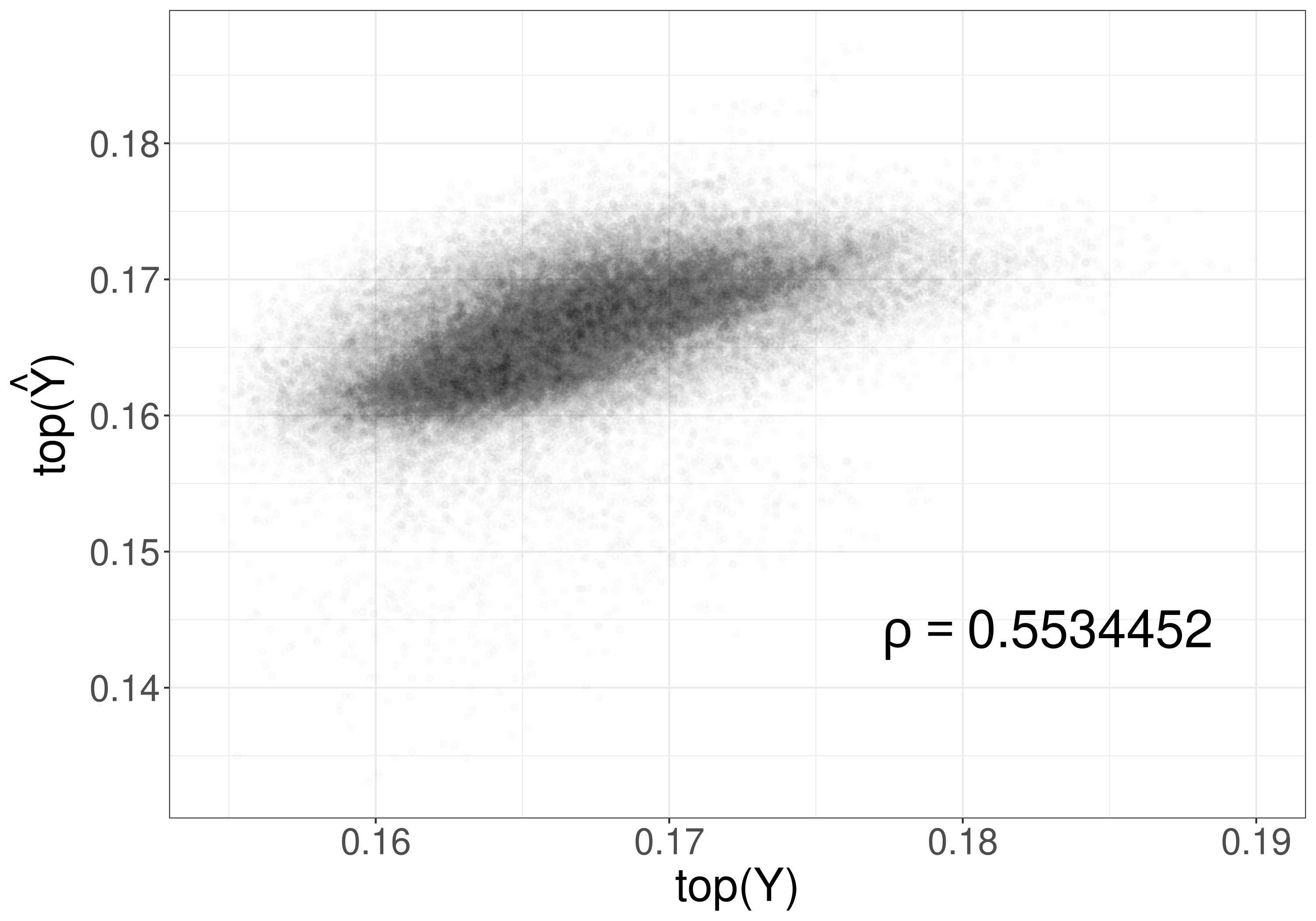
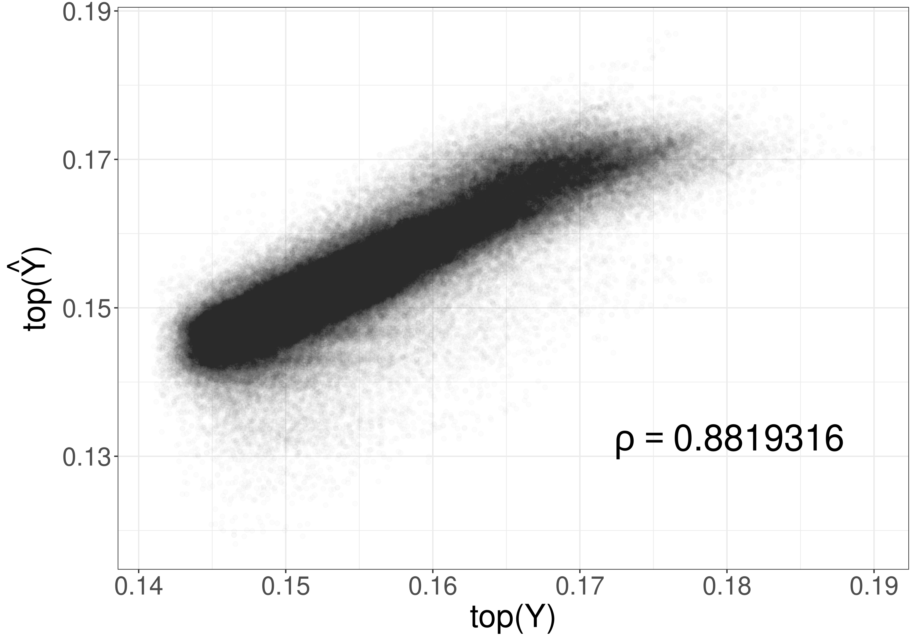
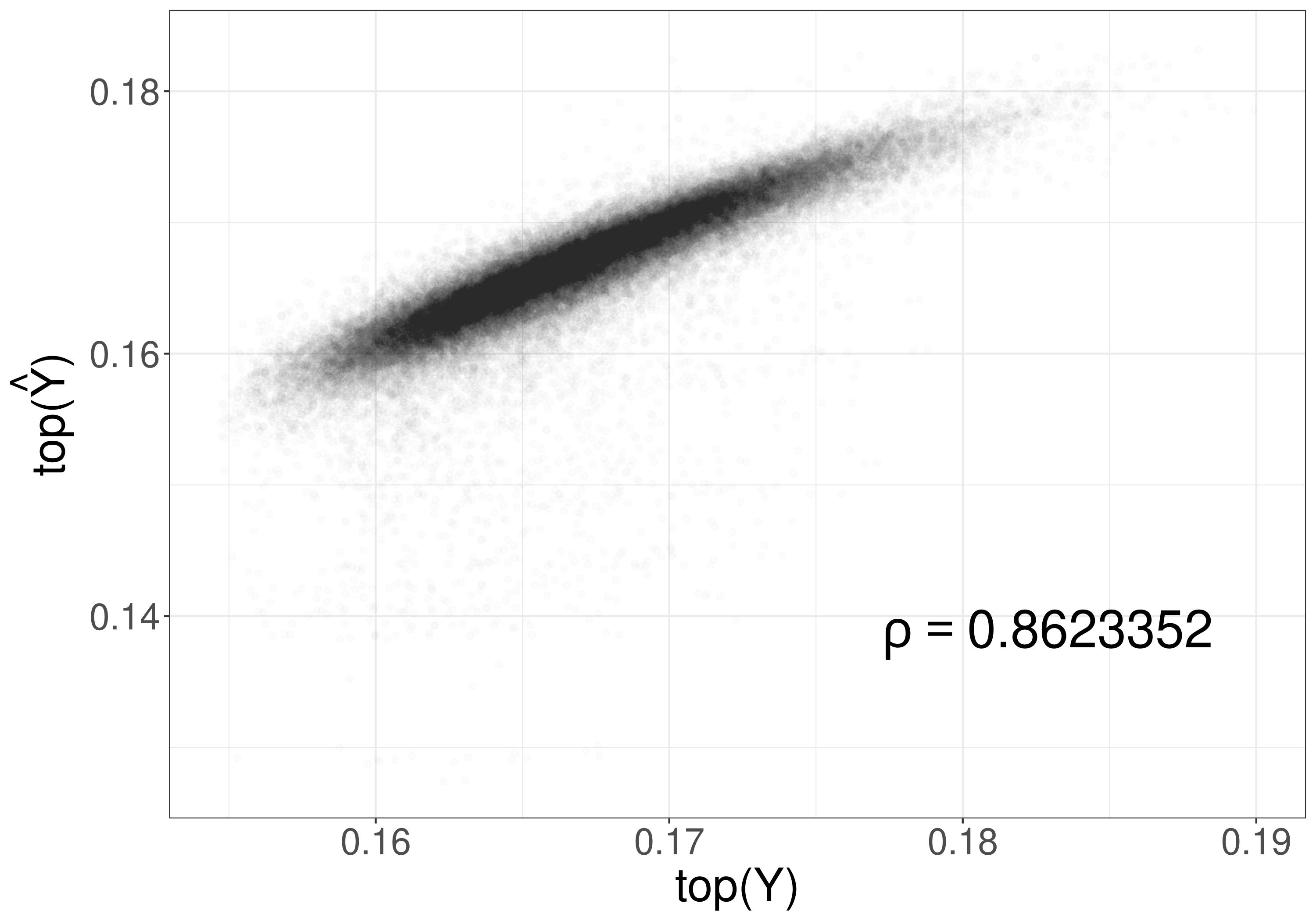
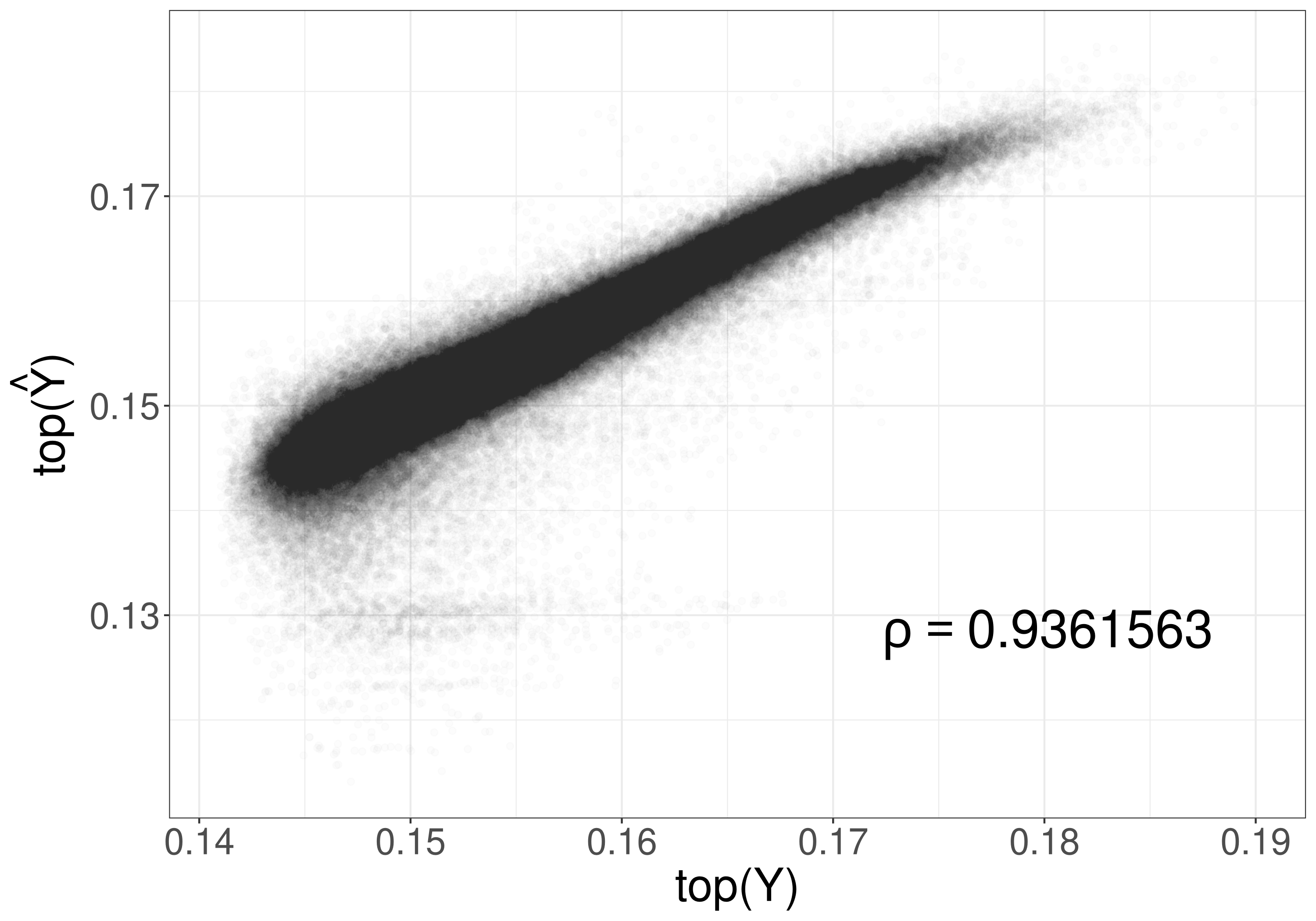
As we see from the two plots at the top the unweighted approach is not well capable to predict high stress values properly - even though there is some correlation present. Bearing in mind that high stress levels correspond to the risk of a highly dangerous rupture of the blood vessel these results are not satisfying. The main reason is the use of a basis for the high fidelity outcome that is not suitable for the compression and prediction of the relevant local high stress parts. The scatterplots for the weighed bases at the bottom show that even though there is a sizable error - most likely due to limited information in the low fidelity outcomes - there is a significant improvement due to the use of weighed basis vectors. This holds despite the fact that the unweighted basis is ten times longer. Points are closer to the diagonal and the average error is lower. Nevertheless, we want to highlight that it remains difficult to predict the highest stress levels.
6 Discussion
This paper proposes dimension reduction utilizing weights corresponding to the relevancy of observations. The starting point is a formula for the projection error using the covariance matrix, which permits a wide range of possible applications. We thereby take advantage of the sparse structure of its inverse, the precision matrix - which follows from the equally sparse neighborhood structure. This allows to numerically solve the resulting optimization problems. Hence, our method only requires numerically treatable covariance structures. Our approach shows advantages in a real world example when predicting high fidelity outcomes from low fidelity simulations. However, it is applicable to other settings as well, where dimension reduction is required but data points differ by relevance, measured by weights.
Appendix
Miscellaneous Numerics
There are a number of crucial numerical concerns that need to be addressed in order to make the basis computation problem laid out in the previous parts solvable in practice. Firstly, we only know the precision matrix, , but not its inverse the GMRF covariance matrix , as seen in (10). , the standard GMRF precision matrix (Rue and Held 2005) is sparse. Moreover, this matrix is not invertible in a strict sense, as the constant vector is an eigenvector with eigenvalue . We can however fix this by adding an identity matrix, i.e. in this work we use
| (19) |
where is a small constant, i.e. and the dimensional identity matrix.
It is not useful nor common to actually invert as this is computationally expensive and results in a dense matrix which consumes a large amount of memory. Instead we compute a sparse Cholesky decomposition which is enough to rapidly compute the matrix / vector operations involving in the formulae for the function value and gradient, like (10) and (11). The decomposition is not sufficient to actually compute the full Hessian matrix as seen in (12). However, this is not necessary as the ability to compute the product of the Hessian with a given vector is sufficient in our case.
There are specialized routines for the case of GMRF type precision matrices which do not only build on the highly sparse nature but also the (up to permutation) band like shape of the matrix in order to achieve a computational cost of up to . This results in a large advantage with regard to computation time in comparison to the ordinary Cholesky decomposition routines which also do not result in sparse matrices. We refer to Davis 2006 as a comprehensive reference. For the computation we use the R package Matrix, which is based on the CHOLMOD (Davis 2021) library. On our machine with GB of RAM and core AMD Ryzen X processor the computation of the decomposition for our dimensional precision matrix takes just seconds.
Low Fidelity Compression Error
Statements and Declarations
No funds, grants, or other support was received.
Additional Material
- Code and Data:
-
full code and data to reproduce the results is available at:
https://drive.google.com/drive/folders/1c68u1bATuOZEIAXuOYzIFb3urSNQwUav?usp=sharing. - Reformulation as Tensor Decomposition:
-
reformulation_tensor_decomposition.pdf contains a reformulation of the first basis vector problem as a tensor decomposition.
- Simulation Study:
-
simulation_study.pdf contains as small simulation study with sampled weight vectors.
References
- Biehler et al. (2014) Biehler J, Gee MW, Wall WA (2014) Towards efficient uncertainty quantification in complex and large-scale biomechanical problems based on a Bayesian multi-fidelity scheme. Biomechanics and Modeling in Mechanobiology 14(3):489–513
- Biehler et al. (2016) Biehler J, Kehl S, Gee MW, Schmies F, Pelisek J, Maier A, Reeps C, Eckstein HH, Wall WA (2016) Probabilistic noninvasive prediction of wall properties of abdominal aortic aneurysms using Bayesian regression. Biomechanics and modeling in mechanobiology
- Davis (2006) Davis TA (2006) Direct Methods for Sparse Linear Systems. Society for Industrial and Applied Mathematics, DOI 10.1137/1.9780898718881, URL https://epubs.siam.org/doi/abs/10.1137/1.9780898718881, https://epubs.siam.org/doi/pdf/10.1137/1.9780898718881
- Davis (2021) Davis TA (2021) Suitesparse. https://github.com/DrTimothyAldenDavis/SuiteSparse, accessed: 2021-09-22
- Gabriel and Zamir (1979) Gabriel KR, Zamir S (1979) Lower rank approximation of matrices by least squares with any choice of weights. Technometrics 21(4):489–498
- Ghojogh et al. (2019) Ghojogh B, Karray F, Crowley M (2019) Eigenvalue and generalized eigenvalue problems: Tutorial. 1903.11240
- Golub et al. (1979) Golub GH, Heath M, Wahba G (1979) Generalized cross-validation as a method for choosing a good ridge parameter. Technometrics 21(2):215–223, DOI 10.1080/00401706.1979.10489751, URL https://www.tandfonline.com/doi/abs/10.1080/00401706.1979.10489751, https://www.tandfonline.com/doi/pdf/10.1080/00401706.1979.10489751
- Li (1986) Li KC (1986) Asymptotic optimality of cl and generalized cross-validation in ridge regression with application to spline smoothing. The Annals of Statistics pp 1101–1112
- Ma et al. (2019) Ma C, Wang K, Chi Y, Chen Y (2019) Implicit regularization in nonconvex statistical estimation: Gradient descent converges linearly for phase retrieval, matrix completion, and blind deconvolution. Foundations of Computational Mathematics 20(3):451–632, DOI 10.1007/s10208-019-09429-9, URL http://dx.doi.org/10.1007/s10208-019-09429-9
- Nocedal and Wright (2006) Nocedal J, Wright SJ (2006) Numerical Optimization, 2nd edn. Springer, New York, NY, USA
- Rue and Held (2005) Rue H, Held L (2005) Gaussian Markov random fields : theory and applications. Chapman & Hall/CRC London
- Soltanpour et al. (2017) Soltanpour S, Boufama B, Jonathan Wu Q (2017) A survey of local feature methods for 3d face recognition. Pattern Recognition 72:391–406, DOI https://doi.org/10.1016/j.patcog.2017.08.003, URL https://www.sciencedirect.com/science/article/pii/S0031320317303072
- Striegel et al. (2022) Striegel C, Biehler J, Wall W, Kauermann G (2022) A multifidelity function-on-function model applied to an abdominal aortic aneurysm. Technometrics pp 1–26, DOI 10.1080/00401706.2021.2024453
- Tamuz et al. (2005) Tamuz O, Mazeh T, Zucker S (2005) Correcting systematic effects in a large set of photometric light curves. Monthly Notices of the Royal Astronomical Society 356:1466 – 1470, DOI 10.1111/j.1365-2966.2004.08585.x
- Xuan (2016) Xuan Y (2016) Rspectra. https://github.com/yixuan/RSpectra/, accessed: 2018-08-09
- Zebari et al. (2020) Zebari R, Abdulazeez A, Zeebaree D, Zebari D, Saeed J (2020) A comprehensive review of dimensionality reduction techniques for feature selection and feature extraction. Journal of Applied Science and Technology Trends 1(2):56–70