Uncertainty Quantification for Fisher-Kolmogorov Equation on Graphs with Application to Patient-Specific Alzheimer Disease Funding: PFA has been partially funded by the research grants PRIN2017 n. 201744KLJL funded by MUR. PFA and AMQ has been partially funded by the research grants PRIN2020 n. 20204LN5N5 funded by MUR. PFA has been partially supported by ICSC—Centro Nazionale di Ricerca in High Performance Computing, Big Data, and Quantum Computing funded by European Union—NextGenerationEU. FB is partially funded by “INdAM - GNCS Project”, codice CUP E53C22001930001. MC, FB, PFA and AMQ are members of INdAM-GNCS.

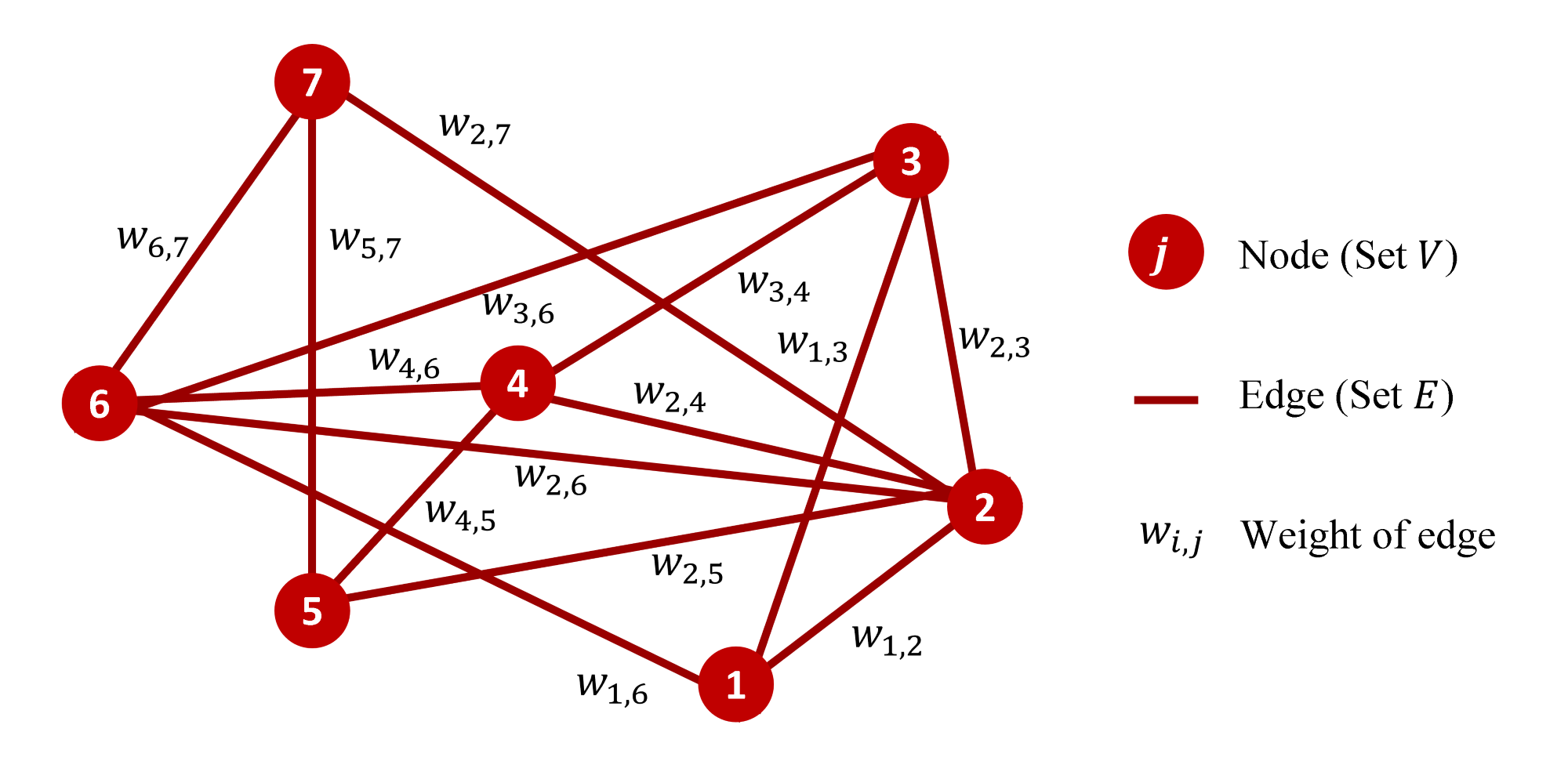
Due to the nature of the prionic diffusion, which is mostly directed as the axonal connections, we discretize Equation (2) on the brain connectome graph, following [21, 8]. More in details, we introduce the graph $\mathscr{G}=(V,E)$ representing a discretization of the domain $\Omega$, where $V=(\boldsymbol{x}_{j})_{j=1}^{M}$ denotes the set of vertices (nodes) of the graph and $E$ denotes the set of edges, as it can be observed in Figure 1.

Applying the theory of discretization of PDEs on graphs [22] to the model problem (2), we find the following semi-discretized formulation

Equation (3) is a system of networked ordinary differential equations (ODEs), where $\mathbf{L}=(\mathbf{L}_{ij})_{i,j=1}^{M}$ denotes the Laplacian matrix that discretizes the continuous Laplacian operator (see [22]), and $c_{j}(t,\boldsymbol{p})\simeq c(\boldsymbol{x}_{j},t,\boldsymbol{p})\colon[0,T]\times\Gamma\rightarrow\mathbb{R}$ is the approximated solution at the $j$-th node $\boldsymbol{x}_{j}$ of the graph $\mathscr{G}$. The solution evaluated at the set of nodes $\boldsymbol{x}_{j}\in V$ is collected into the vector $\boldsymbol{c}=(c_{j})_{j=1}^{M}\colon[0,T]\times\Gamma\rightarrow\mathbb{R}^{M}$. In the same way, the values of the initial condition $c_{0}(\boldsymbol{x})$ at $V$ are collected into the vector $\boldsymbol{c}_{0}=(c_{0j})_{j=1}^{M}\in\mathbb{R}^{M}$, with $c_{0j}=c_{0}(\boldsymbol{x}_{j})$ for all $j=1,\ldots,M$.

To discretize in time, we apply the Crank-Nicolson scheme, with a second-order extrapolation for a semi-implicit treatment of the nonlinear reactive term. In particular, let $\{t_{\ell}\}_{\ell=0}^{N_{t}}$ be the uniform partition of the time interval $[0,T]$ into $N_{t}$ intervals with length $dt=\frac{T}{N_{t}}$, namely, $0=t_{0}<t_{1}<...<t_{N_{t}}=T$ and $t_{\ell}=\frac{\ell T}{N_{t}}$ for $\ell=0,...,N_{t}$. The fully discrete formulation of problem (2) reads: give the initial conditions $\boldsymbol{c}_{0}$ and $\boldsymbol{c}_{-1}$, find $\boldsymbol{c}^{k+1}=\boldsymbol{c}^{k+1}(\boldsymbol{p})$, such that

where $\boldsymbol{\alpha}$ is the vector containing for each node of the graph $\mathscr{G}$, the corresponding value of the reaction parameter $\alpha$, $\boldsymbol{1}$ is a vector of ones and the symbol $\odot$ denotes the (component-by-component) Hadamard product.

As detailed in Section 2, the FK equation (2) depends on the reaction parameter $\boldsymbol{\alpha}(\boldsymbol{x},\boldsymbol{p})$ defined in equation (1). We model it as a stochastic quantity depending on the random vector $\boldsymbol{p}$, because its value encodes many different physical processes that cannot be directly estimated. However, due to the patient-specificity of the neurodegeneration, it is difficult to determine a distribution of the components $(p_{1},\ldots,p_{N})$ that can be used for every patient [13]. For this reason, in this work, we propose to estimate specific distributions of the parameters, starting from the PET medical images and using the MCMC method.

Let us denote with $\mathscr{Q}\in\mathbb{R}$ the QoI or output of the fully-discrete FK formulation (4). It can be seen as a function of the $N$ uncertain parameters, namely $\mathscr{Q}\colon\Gamma\rightarrow\mathbb{R}$, even though generalizations to the vector-valued case are straightforward. Possible examples are the spatial average of the solution at the final time

(see Section 4) or the solution at one specific node $x_{j^{*}}$ at the final time ($\mathscr{Q}(\boldsymbol{p})=c_{j^{*}}(T,\boldsymbol{p}$)).

In order to determine the distribution of the parameter vector $\boldsymbol{p}=(p_{1},\ldots,p_{N})\in\Gamma$, we want to construct a Markov chain, by extracting at every iteration an independent step from a Gaussian distribution $\boldsymbol{\delta}\sim\mathscr{N}(\boldsymbol{0},\widehat{\Sigma})$, where we assume that $\widehat{\Sigma}=\widehat{\sigma}^{2}\mathbf{I}$, with $\widehat{\sigma}$ a scalar value that we assume constant for each parameter of the vector $\boldsymbol{p}$. The idea of the Metropolis-Hastings algorithm is to construct a posterior distribution of the parameter $\pi_{\mathrm{post}}(\boldsymbol{p})$ starting from some assumptions on the prior distributions $\pi_{\mathrm{pr}}(\boldsymbol{p})$ of the parameters. In particular, in this work, we assume a uniform prior distribution of the parameters, with bounds $a_{\ell}$ and $b_{\ell}$ for the $\ell$-th component of the parameters vector $\boldsymbol{p}$.

At each iteration, we choose to accept or not the new value of the chain, by using a Bernoulli distribution of parameter $\rho$, computed using the application of Bayes’ theorem and defined by:

where $\pi(\mathscr{Q}|\boldsymbol{p})$ is the conditioned distribution of the quantity of interest, with respect to the parameters’ realization. The computation of this quantity requires that we assume a model for the uncertainty in the measuring errors. In particular, we can assume that the errors are distributed as a vectorial Gaussian distribution $\mathscr{N}(\boldsymbol{0},\sigma^{2}\mathbf{I})$. In this way, we can obtain a formula for the likelihood distribution:

The MCMC algorithm is reported in Algorithm 1. At the end of the iterations, we compute the vector of the mean $\mu_{\ell}$ and variance $\sigma^{2}_{\ell}$ of the realizations of the $p_{\ell}$ parameter. However, we neglect the first $\widetilde{M}$ realizations, to eliminate the dependency on the initial point of the chain. More information about MCMC methods can be found in [15].

As already discussed in the previous section, FK equation (2) depends on the vector of parameters $\boldsymbol{p}=(p_{1},\ldots,p_{N})\in\Gamma$. The random distribution of each parameter $p_{\ell}$, $\ell=1,\ldots,N$, can be determined following the procedure presented in Section 3.1. In particular, as an output of the inverse UQ problem, we have the set of pairs $\{(\mu_{\ell},\sigma_{\ell})\}_{\ell=1}^{N}$, where each $(\mu_{\ell},\sigma_{\ell})$ denotes the mean and standard deviation of the normal-distributed parameter $p_{\ell}\sim\mathscr{N}(\mu_{\ell},\sigma_{\ell})$. Note that each $p_{\ell}$ takes values in the entire real axes, namely, $\Gamma_{\ell}=\mathbb{R}$, so that $\Gamma=\mathbb{R}^{N}$. Moreover, we denote with $\rho\colon\Gamma\rightarrow\mathbb{R}_{+}$ the joint probability density function (pdf) of $\boldsymbol{p}$. If the entries of $\boldsymbol{p}$ are independent, then there holds $\rho=\prod_{\ell=1}^{N}\rho_{\ell}$, where $\rho_{\ell}\colon\Gamma_{\ell}\rightarrow\mathbb{R}_{+}$ denotes the pdf of a Gaussian random variable $\rho_{\ell}(y)=\frac{1}{\sqrt{2\pi}\sigma_{\ell}}\textrm{exp}\left(\frac{y-\mu_{\ell}}{2\sigma^{2}_{\ell}}\right)$.

In this framework, we are interested in quantifying how the uncertainty in the input parameter vector $\boldsymbol{p}$ affects the QoI, by computing its statistical moments, like the expectation and variance, respectively given by

In particular, in relation to our medical application, we aim at quantifying the impact of varying piecewise constant reaction coefficients of prionic proteins on the onset and progression of Alzheimer disease.

To generate the graph modelling the brain network we employ DWI, a Magnetic Resonance Imaging (MRI), which determines the Brownian motion of the water molecules; indeed the axonal nature of the neuronal connections creates directional paths for the motion. By using DSI studio [20], we can determine the brain’s tractography, highlighting the axons’ principal direction at every point of the brain [25], as we can observe in Figure 2(b).

The tractography is used to derive a weighted graph $\mathscr{G}$, where the nodes in $V$ are associated with a parcellation of the brain regions and the connecting edges $E$ are weighted taking into account both the number of connections and the length of the paths. In this work, we use parcellation based on the Brainnetome Atlas [26] and we group the nodes in $7$ regions: frontal lobe, temporal lobe, parietal lobe, insular lobe, limbic lobe, occipital lobe, and subcortical nuclei. In Figure 2(c) we report the $246$ nodes of the graph coloured according to the corresponding regions, and the edges of the graph are visible in Figure 2(d). We report the local graphs of each region in Figure 3. Moreover, we display the connectogram representing the principal connections between different regions. For readability, the connectogram shows only the principal connections. More specifically, we show the ones associated with weights that are larger than a threshold, which we fix to be equal to the $5\%$ of the maximum weight detected. We underline that the structure of the regions and the graph discretization have a large impact on the parameter calibration and then on the final output of the simulation, as it will be detailed in Section 4.2.

In order to estimate the reaction parameters as well as to set up the initial conditions for the (patient-specific) FK problem, we estimate the concentration $c$ of Amyloid-$\beta$ protein at two different time instances. The medical data used are Positron Emission Tomography images with Pittsburgh compound B (PET-PiB) [4], which uses a radioligand able to identify the presence of Amyloid-$\beta$ plaques (more information on the acquisition techniques of the specific images used in this work can be found in [23]). After having rescaled the values detected by the imaging so that they are between 0 and 1, we average the concentration on the parcellation reconstructed by DSI. Due to the fact that any region of the parcellation is associated with a single node in the brain connectome graph, we are obtaining the values of the concentration $c_{j}$ at any node $j$. The output of the process is the projection of the medical images (at 61 and 68 years of the patient) on the reconstructed graph: see Figure 4(b).

By comparing the two images in Figure 4(b), we notice that the concentration of Amyloid-$\beta$ has increased in the majority of the graph nodes. A more precise comparison is provided in Figure 4(a), where we plot the concentration of the second PET (at 68 years) versus that of the first (at 61 years). Each bullet is coloured according to the region it belongs to (the same color code as in Figure 3 is employed) and its size is proportional to the volume of the represented brain section in the parcellation. The scatter plot confirms the increase of the concentration in most of the nodes. However, it seems that a few nodes exhibit a decrease in the concentration of misfolded proteins. This is non-physical, we also observe that such a non-physical behaviour is mainly located in the subcortical lobe. We attribute this inconsistency to the atrophy of the region, which can be observed in the MRI images around the ventricles, and which is typical of AD [4]. Indeed, a reduction of the tissue can affect the projection of the medical data on the graph, due to the fact that the same pixel of PET image catches a larger part of the domain without neuronal tissue.

In this section, we compute the distributions of the reaction parameters in the 7 regions of the graph by means of the inverse UQ process illustrated in Section 3.1. To better calibrate the distributions, we need to take into account the existence of some outliers in the PET measurements, as explained in Section 4.1. When calibrating the reaction parameters, we will not take into account those nodes at which the concentration in the second PET is lower than in the first one of more than $10\%$.

According to (1), the reaction coefficient $\boldsymbol{\alpha}$ is modelled as a piecewise Gaussian random field, namely, $\boldsymbol{\alpha}$ is a Gaussian random variable whenever restricted to any of the seven brain regions. In particular, we optimize the average concentration of the protein in each region of the graph as follows:

In equation (14) we are computing a weighted average on the $j$-th region of the graph (containing $M_{j}$ nodes), for $j=1,\ldots,7$. The concentration at each node $c^{N_{t}}_{k_{j}}$ is weighted by the volume of the $k_{j}$-th node $v_{k_{j}}$ and divided by the total volume $v_{\mathrm{tot}}$. The corresponding index for each brain region is reported in Table 1.

The Metropolis-Hastings algorithm (see Algorithm 1) is initialized by using a step with standard deviation $\widehat{\sigma}=10^{-2}$. Moreover, we adopt a likelihood with standard deviation $\sigma=0.1$. Finally, we choose the prior distribution for the 7 parameters as $p_{\ell}\sim U(a_{\ell},b_{\ell})$, where $a_{\ell}$ and $b_{\ell}$ are calibrated according to the available medical data (see Table 1).This mean value is also used to initialize the Markov chain, namely $\boldsymbol{p}^{(0)}=\frac{1}{2}(\boldsymbol{a}+\boldsymbol{b})$, where $\boldsymbol{a}=(a_{\ell})_{\ell}$ and $\boldsymbol{b}=(b_{\ell})_{\ell}$. To neglect the impact of the initial choice, we eliminate from the mean and variance computation the first $\widetilde{M}=10\,000$ steps out of the $M=100\,000$ we perform in this simulation.

The output values for $\mu_{\ell}$ and $\sigma^{2}_{\ell}$ are reported in Table 1. We can observe that the mean values feature high variability inside the different regions, and this result justifies the choice of using a non-homogeneous spatial description of the corresponding parameter. Moreover, in Figure 5 we display the 7 different estimated distributions with the histograms associated with the Markov chain realizations. We can observe coherence between the result of the MCMC algorithm and the resulting Gaussian probability distributions, that we use in the following section. Finally, in Figure 5 we report the comparison between the $\mathscr{Q}$ computed starting from the numerical solution, obtained using the mean values of the parameters and the corresponding $\mathscr{Q}$ derived from the medical images, neglecting the outliers as explained in Section 4.1. In the results reported in Figure 5 the size of the bullets is proportional to the volume of the lobes. The accuracy of the estimating algorithm for the parameters can be measured by the distance from the bisecting line, in which the numerical predicted value would be exactly equal to the medical data from PET images. Finally, we report the numerical solution on the graph and the medical data at the final time. In both cases, we observe a higher concentration of misfolded proteins inside the parietal and frontal lobes, coherently to what we expect from the medical literature [27]. This shows that our numerical method is able to reproduce the disease progression.

In this section, we simulate future scenarios of the development of the Amyloid-$\beta$ concentration inside the brain, by following the two approaches presented in Section 3.2, namely MC and SC.

In this simulation, we fix the final time at $T=20\,\mathrm{years}$ and we discretize the time interval $[0,T]$ with a timestep $dt=0.02\,\mathrm{years}$ (we denote the set of all considered time instances as $\mathscr{I}_{T}$). As QoI we choose the spatial average of the concentration inside the seven lobes of the brain graph, evaluated at all time instances $t\in\mathscr{I}_{T}$. In particular, at every $t\in\mathscr{I}_{T}$, we have a vectorial QoI $\mathscr{Q}=(\mathscr{Q}_{1},\ldots,\mathscr{Q}_{7})$, where the $j$-th component is $\mathscr{Q}_{j}=\langle c_{h}\rangle_{j}(t)$ for $j=1,...,7$. We aim at approximating the expected value and the variance of each of the QoI.

The reference expectation and variance are computed using the SC method on a Smolyak sparse grid of level 9 with Leja points (in total, there are $224\,143$ collocation nodes). The reference expectation and variance are denoted by $\boldsymbol{\mu}_{Q}$ and $\boldsymbol{\sigma}_{Q}^{2}$, respectively, and they are both vectors of length $7$: their different components correspond to the regions of the brain graph. In Figure 6(a), we report the computed results in terms of the volume-weighted mean value over the different lobes $\langle\boldsymbol{\mu}_{Q}\rangle$ and a range of standard deviation $[\langle\boldsymbol{\mu}_{Q}\rangle-\langle\boldsymbol{\sigma}_{Q}\rangle;\langle\boldsymbol{\mu}_{Q}\rangle+\langle\boldsymbol{\sigma}_{Q}\rangle]$. We observe a global increase of prionic concentration in time, coherently to what expected by the disease progression [27]. Moreover, the stochastic description yields an increasing uncertainty over the years, which allows for obtaining a range of future possible scenarios after many years.

We perform a convergence analysis, with the aim of assessing the approximation properties of Smolyak sparse grids with increasing level $w=3,4,5,6,7,8$. The errors are reported in Table 2. We can notice that both for $\langle\boldsymbol{\mu}_{Q}\rangle$ and $\langle\boldsymbol{\sigma}^{2}_{Q}\rangle$, we have a monotone decrease of the error as the number of collocation points increases. We can also notice, that the accuracy of the approximation deteriorates as time advances. Indeed, it is reasonable that it is necessary to use a larger number of points, to approximate phenomena with larger variance, such as the concentration after 15-20 years. The convergence results for the SC method are also displayed in Figures 6(b) and 6(c), where the errors at time instances $t=5,10,15,20$ are reported versus the number of collocation points. For the sake of comparison, we also report the convergence of the MC error versus the number of MC samples (note that the MC error decays with the predicted rate $M^{-1/2}$, $M$ being the number of samples). We notice that, with a comparable number of evaluations of the differential problem, the SC method provides a more accurate solution. This is particularly pronounced for smaller time instances.

References

- [1] L. C. Walker and M. Jucker, “Neurodegenerative diseases: Expanding the prion concept,” Annual Review of Neuroscience, vol. 38, no. 1, pp. 87–103, 2015.
- [2] P. Scheltens, B. De Strooper, M. Kivipelto, H. Holstege, G. Chételat, C. E. Teunissen, J. Cummings, and W. M. van der Flier, “Alzheimer’s disease,” The Lancet, vol. 397, pp. 1577–1590, 2021.
- [3] G. S. Bloom, “Amyloid- and tau: the trigger and bullet in Alzheimer disease pathogenesis,” JAMA neurology, vol. 71, no. 4, pp. 505–508, 2014.
- [4] W. M. van Oostveen and E. C. M. de Lange, “Imaging Techniques in Alzheimer’s Disease: A Review of Applications in Early Diagnosis and Longitudinal Monitoring,” International Journal of Molecular Sciences, vol. 22, no. 4, p. 2110, 2021.
- [5] H. Hampel, K. Bürger, S. J. Teipel, A. L. W. Bokde, H. Zetterberg, and K. Blennow, “Core candidate neurochemical and imaging biomarkers of Alzheimer’s disease,” Alzheimer’s & Dementia: The Journal of the Alzheimer’s Association, vol. 4, no. 1, pp. 38–48, 2008.
- [6] B. Franchi and S. Lorenzani, “From a microscopic to a macroscopic model for Alzheimer disease: Two-scale homogenization of the Smoluchowski equation in perforated domains,” Journal of Nonlinear Science, vol. 26, p. 717–753, 2016.
- [7] J. Weickenmeier, M. Jucker, A. Goriely, and E. Kuhl, “A physics-based model explains the prion-like features of neurodegeneration in Alzheimer’s disease, Parkinson’s disease, and amyotrophic lateral sclerosis,” Journal of the Mechanics and Physics of Solids, vol. 124, pp. 264–281, 2019.
- [8] S. Fornari, A. Schäfer, M. Jucker, A. Goriely, and E. Kuhl, “Prion-like spreading of Alzheimer’s disease within the brain’s connectome,” Journal of The Royal Society Interface, vol. 16, no. 159, p. 20190356, 2019.
- [9] A. Schäfer, J. Weickenmeier, and E. Kuhl, “The interplay of biochemical and biomechanical degeneration in Alzheimer’s disease,” Computer Methods in Applied Mechanics and Engineering, vol. 352, pp. 369–388, 2019.
- [10] M. Corti, P. F. Antonietti, F. Bonizzoni, L. Dede’, and A. M. Quarteroni, “Discontinuous Galerkin methods for Fisher-Kolmogorov equation with application to -synuclein spreading in Parkinson’s disease,” arXiv:2302.07126, 2023.
- [11] F. Bonizzoni, M. Braukhoff, A. Jüngel, and I. Perugia, “A structure-preserving discontinuous Galerkin scheme for the Fisher–KPP equation,” Numerische Mathematik, vol. 146, no. 1, pp. 119–157, 2020.
- [12] A. Goriely, E. Kuhl, and C. Bick, “Neuronal oscillations on evolving networks: Dynamics, damage, degradation, decline, dementia, and death,” Physical Review Letters, vol. 125, no. 12, p. 128102, 2020.
- [13] A. Schäfer, M. Peirlinck, K. Linka, E. Kuhl, and ADNI, “Bayesian Physics-Based Modeling of Tau Propagation in Alzheimer’s Disease,” Frontiers in Physiology, vol. 12, p. 1081, 2021.
- [14] A. Schäfer, P. Chaggar, A. Goriely, E. Kuhl, and ADNI, “Correlating tau pathology to brain atrophy using a physics-based Bayesian model,” Engineering with Computers, vol. 38, no. 5, pp. 3867–3877, 2022.
- [15] C. P. Robert and G. Casella, Monte Carlo Statistical Methods. Springer, 2 ed., 1999.
- [16] W. K. Hastings, “Monte Carlo Sampling Methods Using Markov Chains and Their Applications,” Biometrika, vol. 57, no. 1, pp. 97–109, 1970.
- [17] J. H. Halton, “A Retrospective and Prospective Survey of the Monte Carlo Method,” SIAM Review, vol. 12, no. 1, pp. 1–63, 1970.
- [18] I. Babuška, F. Nobile, and R. Tempone, “A Stochastic Collocation Method for Elliptic Partial Differential Equations with Random Input Data,” SIAM Journal on Numerical Analysis, vol. 45, no. 3, pp. 1005–1034, 2007.
- [19] F. Nobile, R. Tempone, and C. G. Webster, “A Sparse Grid Stochastic Collocation Method for Partial Differential Equations with Random Input Data,” SIAM Journal on Numerical Analysis, vol. 46, no. 5, pp. 2309–2345, 2008.
- [20] “DSI-Studio: A Tractography Software Tool for Diffusion MRI Analysis.” https://dsi-studio.labsolver.org/.
- [21] R. F. Betzel and D. S. Bassett, “Generative models for network neuroscience: Prospects and promise,” Journal of The Royal Society Interface, vol. 14, no. 136, p. 20170623, 2017.
- [22] A. J. Smola and R. Kondor, “Kernels and Regularization on Graphs,” in Learning Theory and Kernel Machines, pp. 144–158, Springer, 2003.
- [23] P. J. LaMontagne, T. L. Benzinger, J. C. Morris, S. Keefe, R. Hornbeck, C. Xiong, E. Grant, J. Hassenstab, K. Moulder, A. G. Vlassenko, M. E. Raichle, C. Cruchaga, and D. Marcus, “Oasis-3: Longitudinal neuroimaging, clinical, and cognitive dataset for normal aging and alzheimer disease,” medRxiv, 2019.
- [24] C. Piazzola and L. Tamellini, “The Sparse Grids Matlab kit – a Matlab implementation of sparse grids for high-dimensional function approximation and uncertainty quantification,” arXiv:2203.09314, 2022.
- [25] F.-C. Yeh, “Shape analysis of the human association pathways,” NeuroImage, vol. 223, p. 117329, 2020.
- [26] L. Fan, H. Li, J. Zhuo, Y. Zhang, J. Wang, L. Chen, Z. Yang, C. Chu, S. Xie, A. R. Laird, P. T. Fox, S. B. Eickhoff, C. Yu, and T. Jiang, “The Human Brainnetome Atlas: A New Brain Atlas Based on Connectional Architecture,” Cerebral Cortex, vol. 26, no. 8, pp. 3508–3526, 2016.
- [27] H. Hampel, J. Hardy, K. Blennow, C. Chen, G. Perry, S. H. Kim, V. L. Villemagne, P. Aisen, M. Vendruscolo, T. Iwatsubo, C. L. Masters, M. Cho, L. Lannfelt, J. L. Cummings, and A. Vergallo, “The Amyloid- Pathway in Alzheimer’s Disease,” Molecular Psychiatry, vol. 26, no. 10, pp. 5481–5503, 2021.
- [28] S. Salsa, Partial Differential Equations in Action: from Modeling to Theory. Springer, 3 ed., 2016.