Emulation Learning for Neuromimetic Systems

The work being reported continues our effort to develop the theoretical foundations of control system designs that exhibit key features of the neural mechanisms that govern movement and other behaviors in animals. One such feature is control modulation involving actions of very large numbers of simple inputs and outputs that are effective in influencing the system dynamics only in their aggregate operation. The goal of research on such control systems is to understand the engineering analogs of neuroplasticity, learning and relearning, memory and adaptation. Previously reported work has introduced what we call neuromimetic linear models. The focus has been on finite dimensional linear systems that are overcomplete in that they have many more input and output channels than the dimension of the state [1],[6]. Such systems have been shown to have reduced cost of operation in terms of standard $L_{2}$ metrics, reduced uncertainty in the face of input channel noise, and resilience with respect to drop-outs of input or output channels, [9]. With such qualities in mind, research is now aimed at overcomplete models with simple neuron-like discrete inputs taking values $\{-1,0,1\}$ and exploring how well these are able to emulate the behaviors of systems with standard continuous feedback designs. In [10], algorithms based on ideas from machine learning were used to solve a restricted emulation problem. The solutions were useful in comparing optimal and nearby suboptimal designs as well as in suggesting approaches to understanding the complexity of neuromimetic feedback designs.

One of the approaches to feedback control using the quantized control inputs of [10] involved reinforcement learning (RL)–specifically, a DQN-like algorithm [11],[12]. RL can solve continuous decision-making tasks remarkably effectively. Agents can improve their performance by interacting with the environment through trial-and-error to minimize an emulation error metric [2]. However, when the state and action sets become large or possibly infinite, tabular solution methods must be abandoned in favor of approaches that lead only to approximate solutions. The approach here, following basic ideas from [11], is to replace the Q-table of basic RL with a deep Q neural network (DQN). Revisiting [5] in what follows, we examine the inherent complexity arising from the set of state-action pairs being infinite and the decision space being discrete. Even in this somewhat simple case, obtaining a sufficient sample of interactions as the emulation problem under study changes remains challenging since it is a time-sensitive problem, [7]. For this reason, we consider transfer learning (TL) [3] as a way to utilize the experience from other emulation problems to accelerate the learning process for the new problem, [8].

The rest of the paper is organized as follows. Section II describes the emulation problems, our system models, and the design goals of the learning algorithm. Section III introduces two approaches: an MPC-data based learning method and a generalized deep Q-network (DQN). Section IV presents the transfer learning algorithm to adapt the learned model a new emulation problem. Section V shows simulation results that illustrate the proposed approaches, and we make a summary in Section VI.

Consider the linear time-invariant (LTI) systems of the form

By applying the simple feedback control law $u=Kx$, where $K$ is a stabilizing gain chosen as in [10], we obtain the closed-loop LTI system

where $H=A+BK\in\mathbb{R}^{n\times n}$ is Hurwitz. Following [9], [10], we consider the problem of emulating (2) by means of a discrete-time system with quantized inputs

where $x_{qs}\in\mathbb{R}^{n}$ is the system state, $u\in\mathbb{U}=\{-1,0,1\}^{m}$ is the set of possible quantized inputs. Following [10], we refer to these inputs $u(k)$ as activation patterns. $h$ is the time step and $m\gg n$ denotes the large number of input channels. Here we provide an example.

Consider solutions to the linear ordinary differential equation (ODE) (2). The goal of the general emulation problem is to find piecewise constant quantized inputs with sampling interval $h>0$ such that the resulting trajectories of (3) with initial state $x_{qs}(0)=x_{0}$ approximate the continuous system $(\ref{equation:LTI})$. Here, we solve the emulation problem that finds a partition of the state space $\{U_{i}\,:\,\cup\ U_{i}=\mathbb{R}^{n};\ \ U_{i}^{o}\cap U_{j}^{o}=\emptyset;\ U_{i}^{o}={\rm interior}\ U_{i}\}$ and a selection rule depending on the current state $x_{qs}(k)$ for assigning values of the input at the $k$-th time step to be $u(k)\in{\cal U}=\{-1,0,1\}^{m}$, so that for each $x_{qs}\in U_{i}$, $e^{Ah}x_{qs}(k)+\int_{0}^{h}e^{A(h-s)}dsBu(k)$ is as close as possible to the emulated LTI system. We have defined various metrics in terms of which we determine the fitness of an approximation such as the direction and magnitude between two systems as was studied in [9]. When $m$ is large ($B$ is $n\times m$ with $m\gg n$), it will frequently be the case that several activation patterns have comparable fitness. Because two or more activation patterns may give approximately equal quality of emulation, it may be the case that over the course of a trajectory, we need to consider multi-step fitness. This is illustrated in the Fig.1, where we see that the red approximants have the best first vector step matching the vectorfield (black vector), but in considering pairs of steps, the blue pair of vectors end up closer to the black pair than the red. Hence, when applying algorithms to learn to optimally emulate a given system, we need to focus on methods that consider multiple steps, and we need to be aware that there may be multiple solutions of approximately equal value.

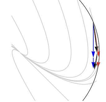
Our goal is to design algorithms that can meet the following objectives:

• •

  Quantized system (3) can emulate the LTI system (2), i.e., at any given point, the model generated by the algorithm can compute an optimal quantized direction taking into account multiple steps.

• •

  The emulation task can still be achieved when there are channel dropouts in the quantized system during the emulating process.

• •

  When the emulated LTI system has changed, the model still works well under new circumstances directly without the need of retraining.

For emulation learning of trajectories of a given LTI system, we propose two approaches: an MPC data-based supervised learning approach that trains a neural network using training data collected from solving the MPC optimization problem and a generalized DQN algorithm by exploring the environment. We shall discuss the advantages of these approaches in terms of the optimality of trajectory, computational efficiency and resilience to channel dropouts.

In addition to the ability to learn, neurobiological system have the ability to generalize and adapt what they have learned to new but similar problem domains. To explore such transfer learning in the context of our emulation problems, suppose that a DQN has been trained for emulating a particular LTI system. Suppose another LTI system has the form

and $H_{o}=OHO^{-1}$ where $O$ is known and invertible. To emulate this LTI system, we utilize a mapping-based transfer learning method [13]. The coordinate is transformed by setting $z=Ox$, then the dynamic equations of these two LTI systems have the following relation:

Assume we have already obtained a trained model from the MPC data-based or the DQN-like algorithm for the emulation problem of (2) using (3), say $F:\mathbb{R}^{2n}\rightarrow\mathbb{R}^{n}$, which is expressed by a neural network. $2n$ is the dimension of state $s$ and $n$ is the dimension of the quantized direction $d$. The model can predict the optimal quantized direction at any given state $s$. For example, $d=\arg\max\limits_{d}Q^{*}_{\phi}(s,d)$ if the DQN model is used.

Instead of learning $F_{o}$ by constructing another dataset by solving a new MPC problem or learning a new deep Q network—which are time-consuming, we try to obtain a selection policy $F_{o}$ from $F$. The strategy will be to use mapping-based transfer learning, [12]. The main idea is to express the relationship of features. Therefore, $F$ can be used directly by the following steps to obtain the learned policy $F_{o}$:

• •

  Record the learning metric like the error vector between the new LTI system (15) and the quantized system (3) as feature $f_{1}\in\mathbb{R}^{n}$, the direction (i.e., $[x(k+1)-x(k)]/h$) or the location of the LTI system (i.e., $x(k)$) as feature $f_{2}\in\mathbb{R}^{n}$. Combine these features to be $f_{o}=[f_{1};f_{2}]\in\mathbb{R}^{2n}$;

• •

  Transform the coordinate of features $f_{o}$ to the coordinate system of (2): $f=\begin{bmatrix}O^{-1}&0\\ 0&O^{-1}\end{bmatrix}{f_{o}}$;

• •

  Predict the optimal direction by $\vec{d}=F(f)$;

• •

  Change back the predicted direction to the coordinate system of (15): $\vec{d_{o}}=O\vec{d}$. It is noted that $\vec{d_{o}}$ may not be in the quantized direction set formed in the current coordinate;

• •

  Find the nearest neighbor of $\vec{d_{o}}$ in the direction set by kd-tree or Hebbian-Oja algorithm [10], and denote this by $\vec{d^{*}}$.

• •

  It is the (sub)optimal output direction for emulating the system (15).

In this section, we provide simple simulations of the learned trajectory per the MPC-based method and per the DQN algorithm. The LTI system we try to emulate is $\dot{x}=Hx=\begin{bmatrix}0&1\\ -1&-2\end{bmatrix}x$ with all its eigenvalues located in the left-half plane. To simplify the example, we set $A$ and $B$ be as in Example 1 and choose time step $h=0.05$. In the cost function, we design $P=Q=\begin{bmatrix}5&0\\ 0&5\end{bmatrix}$ and $R$ to be $0.05*\mathbb{I}_{m}$. The result is shown in Fig. 4(a). It can be observed that by solving the MPC optimization problem (III-A), we generate a sequence of vector steps that emulate the LTI system moving towards the origin.

At the same time, we collect a total of 10000 data points with error vector, i.e., $x(k)-x_{qs}(k)$ and directions, i.e., $[x(k+1)-x(k)]/h$ and $[x_{qs}(k+1)-x_{qs}(k)]/h$ of two systems as features, and quantized directions as their labels. Then, we construct a regular densely-connected four-layer neural network with ReLU, Sigmoid, or Linear as their activation functions. The number of nodes in each layer is 1200, 1200, 1200, and 25, respectively. After 20 training epochs, we obtain a model with a training accuracy of 94.1%. The test dataset comes from another emulation with all initial points in the unit circle, which contains 840 data points, and the accuracy is 90.7%. The trajectory generated by this model is shown in Fig. 4(b).

Using the same $A,B$ matrices and the same emulated system, we also construct a two linear-layer $Q$ network with a hidden layer with 200 activation units between them to learn the trajectory. The activation function is ReLU. Fig. 5(a) is an emulating system produced by the generalized DQN algorithm. The learning metric in the algorithm only considers the $L_{2}$ norm of the error vector between two systems. At time $T$, the location of the LTI system is $x(T)=e^{THh}x_{0}$, while the quantized system is in the location $x_{qs}(T)=x_{0}+hBu(0)+hBu(1)+\cdots+hBu(T-1)$. Therefore, $G(u,T)=||e^{THh}x_{0}-(x_{0}+hB\sum_{t=0}^{T-1}u(t))||^{2}$, where $x_{0}$ is the initial point. In this simple example, there are 25 distinct directions (including zero vector) in the quantization output alphabet formed by $Bu$, where $u_{i}\in\{-1,0,1\}^{4}$. Fig. 5(b) provides an example of having one channel randomly dropout at each time instant. Though it has degraded performance, it still has the ability to emulate.

Next, we use the mapping-based transfer learning method to emulate another LTI system $\dot{z}=H_{o}z=\begin{bmatrix}-2&1\\ -1&0\end{bmatrix}z$. The transform matrix is $O=\begin{bmatrix}0&1\\ -1&0\end{bmatrix}$ in (16), which results in the action space being invariant. The models we use are the MPC data-based learning and the DQN-like algorithm, respectively. The tracking performance is shown in Fig. 6. It illustrates that both of these two models can be transferred to solve another emulation problem.

When the transform matrix is $O=\begin{bmatrix}1&0.5\\ -0.5&1\end{bmatrix}$ in (16), the action space is no longer invariant as is illustrated in Fig. 7(a). The red vector directions form the new action space, used in emulating a new LTI system. For this example, the new emulated LTI system is $\dot{z}=H_{o}z=\begin{bmatrix}-0.5&0\\ -1&-2.5\end{bmatrix}z$. The model we used is the DQN-like Algorithm 1 and the tracking performance is shown in Fig. 7(b).

To compare the training time of the model with initial weights and the existing model obtained from the previous emulation problem, we still choose the new emulated LTI system to be $\dot{z}=H_{o}z=\begin{bmatrix}-0.5&0\\ -1&-2.5\end{bmatrix}z$. The existing DQN model is obtained from emulating the LTI system $\dot{x}=Hx=\begin{bmatrix}0&1\\ -1&-2\end{bmatrix}x$, which generates the trajectory of Fig.5(a). Then, we train 20 episodes of these two models, respectively. Simulation results are shown in Fig. 8. It can be observed that the existing model has a better emulation performance after the same training episodes. The reason is that borrowing the existing model’s structure and parameters for the new problem can reduce the value of the loss function to a certain extent during the initial training to shorten the training time.

The work we have reported examines techniques in machine learning by which the neuromimetic linear models introduced in [9] and [10] can learn to emulate stable closed-loop systems. We have proposed a learning model incorporating model predictive control (MPC) as well as a custom deep Q network (DQN) algorithm. For both approaches, we have studied specific cases in which transfer learning is possible for systems related by certain classes of coordinate transformations. For all cases, it is noted that the kinds of resilience to channel dropouts reported previously persist in the learned models. Future work will be aimed at showing how a continuous observer can be used to synthesize quantized trajectories for the class of overcomplete systems under consideration.

References

- [1] J. Baillieul and Z. Kong, “Saliency based control in random feature networks,” in 53rd IEEE Conference on Decision and Control’, Los Angeles, CA, 2014, pp. 4210-4215. doi: 10.1109/CDC.2014.7040045
- [2] R. S. Sutton and A. G. Barto, Reinforcement learning: An introduction. MIT press, 2018.
- [3] A. Lazaric, “Transfer in reinforcement learning: a framework and a survey.” in Reinforcement Learning: State-of-the-Art, Springer, 2012.
- [4] R. Bellman, “A markovian decision process,” Journal of mathematics and mechanics, 1957.
- [5] K. Arulkumaran, M. P. Deisenroth, M. Brundage, and A. A. Bharath, “A brief survey of deep reinforcement learning,” arXiv preprint arXiv:1708.05866, 2017.
- [6] J. Baillieul, ”Perceptual Control with Large Feature and Actuator Networks,” 2019 IEEE 58th Conference on Decision and Control (CDC), Nice, France, 2019, pp. 3819-3826, doi: 10.1109/CDC40024.2019.9029615.
- [7] Zhu, Z., Lin, K. and Zhou, J., ”Transfer learning in deep reinforcement learning: A survey”, arXiv preprint arXiv:2009.07888, 2020.
- [8] S. J. Pan and Q. Yang, “A survey on transfer learning,” IEEE Transactions on knowledge and data engineering, 2009.
- [9] J. Baillieul and Z. Sun, “Neuromimetic Control–A Linear Model Paradigm,” 2021 60th IEEE Conference on Decision and Control (CDC), 2021, pp. 2709-2716, doi: 10.1109/CDC45484.2021.9683392.
- [10] Z. Sun, and J. Baillieul. ”Neuromimetic Linear Systems—Resilience and Learning.” 2022 IEEE 61st Conference on Decision and Control (CDC), pp. 7388-7394. IEEE, 2022.
- [11] Mnih, V., Kavukcuoglu, K., Silver, D. et al. Human-level control through deep reinforcement learning. Nature 518, 529–533 (2015). https://doi.org/10.1038/nature14236
- [12] Matteo Hessel, Joseph Modayil, Hado Van Hasselt, Tom Schaul, Georg Ostrovski, Will Dabney, Dan Horgan, Bilal Piot, Mohammad Azar, and David Silver. Rainbow: Combining improvements in deep reinforcement learning. In Thirty-Second AAAI Conference on Artificial Intelligence, 2018.
- [13] C. Tan, F. Sun, T. Kong, W. Zhang, C. Yang, and C. Liu. ”A survey on deep transfer learning.” In Artificial Neural Networks and Machine Learning–ICANN 2018: 27th International Conference on Artificial Neural Networks, Rhodes, Greece, October 4-7, 2018, Proceedings, Part III 27, pp. 270-279. Springer International Publishing, 2018.
- [14] John N Tsitsiklis and Benjamin Van Roy. An analysis of temporal-difference learning with function approximation. IEEE transactions on automatic control, 42(5):674–690, 1997.
- [15] Hado Van Hasselt, Yotam Doron, Florian Strub, Matteo Hessel, Nicolas Sonnerat, and Joseph Modayil. Deep reinforcement learning and the deadly triad. arXiv preprint arXiv:1812.02648, 2018.
- [16] S. El-Tantawy, B. Abdulhai, and H. Abdelgawad, “Multiagent reinforcement learning for integrated network of adaptive traffic signal controllers (marlin-atsc): methodology and large-scale application on downtown toronto,” IEEE Transactions on Intelligent Transportation Systems, 2013.
- [17] Z. Sun, and J. Baillieul. ”Model Predictive Control for Neuromimetic Quantized Systems.” arXiv preprint arXiv:2212.09887, 2022.
- [18] E. Oja, “Simplified neuron model as a principal component analyzer,” 1982. Journal of Mathematical Biology, 15(3), pp.267-273.
- [19] Wang, Z.T. and Ueda, M., 2021. Convergent and efficient deep Q network algorithm. arXiv preprint arXiv:2106.15419.
- [20] Sergey Levine, Peter Pastor, Alex Krizhevsky, Julian Ibarz, and Deirdre Quillen. Learning hand- eye coordination for robotic grasping with deep learning and large-scale data collection. The International Journal of Robotics Research, 37(4-5):421–436, 2018.
- [21] Christopher John Cornish Hellaby Watkins. Learning from delayed rewards. 1989.