Towards Causal Representation Learning and Deconfounding from Indefinite Data
Abstract
Owing to the cross-pollination between causal discovery and deep learning, non-statistical data (e.g., images, text, etc.) encounters significant conflicts in terms of properties and methods with traditional causal data. To unify these data types of varying forms, we redefine causal data from two novel perspectives and then propose three data paradigms. Among them, the indefinite data (like dialogues or video sources) induce low sample utilization and incapability of the distribution assumption, both leading to the fact that learning causal representation from indefinite data is, as of yet, largely unexplored. We design the causal strength variational model to settle down these two problems. Specifically, we leverage the causal strength instead of independent noise as the latent variable to construct evidence lower bound. By this design ethos, The causal strengths of different structures are regarded as a distribution and can be expressed as a 2D matrix. Moreover, considering the latent confounders, we disentangle the causal graph into two relation subgraphs and . contains pure relations between observed variables, while represents the relations from latent variables to observed variables. We implement the above designs as a dynamic variational inference model, tailored to learn causal representation from indefinite data under latent confounding. Finally, we conduct comprehensive experiments on synthetic and real-world data to demonstrate the effectiveness of our method.
1 Introduction
Identifying causal relationships from observed data, known as Causal Discovery, has drawn much attention in the fields leveraging substantial statistical datasets, such as the CPRD [11], the DWD Climate [8] and AutoMPG [2]. However, in light of the recent advances in deep learning, particularly in LLMs, there is a growing tendency to incorporate causal discovery in more complex forms of data, including images [9], text [5], and videos [22].
These data, sourced from various modalities and non-statistical, have lacked a unified definition due to their intricate characteristics and complex structures [25]. For instance, the Netsim dataset [29] introduced 50 distinct causal structures. When conventional methods [33, 30, 6] are extended to the Netsim dataset, they have to refit a new probabilistic model to account for a set of new samples whenever the causal structure does not hold. Another example is the IEMOCAP dataset [4], wherein the causal variables are text type and cannot be directly represented numerically. In computations, these are often quantified using multi-dimensional deep representation (word embeddings). Unlike traditional datasets containing statistical data such as body temperature, blood pressure, wind strength, etc., capitalizing on conventional methods like conditional independence [30], regression residual [36], or rank of covariance [31], prove challenging for such deep representation due to their dimension values’ interdependencies.
Hence, trying to give an unified redefinition of both emerging datasets and the traditional ones, we, from a new perspective, utilize the skeleton quantity to represent the number of involved causal sturctures and adopt the dimensionality of the causal representation to gauge the complexity of the one causal variable. The distinction between multi-skeleton () and single-skeleton () lies in whether multiple causal structures exist within a dataset. Simultaneously, the difference between multi-value () and single-value () depends on whether the causal variables are deep representations or not.
Consequently, we categorize causal data into three data paradigms systematically: Definite data characterized by a single-skeleton structure () and single-value variables (); Semi-definite data characterized either by a single-skeleton structure () and multi-value variables (), or by multi-skeleton structures () and single-value variables (); and Indefinite data characterized by multi-skeleton structures () and multi-value variables ().
On the extreme end, a number of methods have been proposed to address these two challenges, but all of them face diverse limitations. For example, to ameliorate the problem of multi-skeleton structures, some methods [7, 13, 19] account for different structures by learning the dynamics across all samples, which can infer causal relations in previously unseen samples without refitting the model. However, these methods impose a stringent assumption of a stationary number of observed nodes which is often violated in many applications. Moreover, to model multi-value nodes, existing methods [5, 9, 35] seek to learn a causal representation via auto regression model while ignoring the effect of latent confounders.
Towards causal representation learning and deconfounding from multi-skeleton and multi-value data, We designed a novel dynamic variational framework. Specifically,
i) We designed a variational model with the causal strength matrix as the latent variable. Comparing with the conventional method which adopts noise matrix as the latent variable, it has significant superiority in processing multi-skeleton and multi-value data.
ii) We adopted the individual-specific effects on each observed node instead of estimation on latent variables to probe latent confounding. Under this observe-node-oriented representation, we can disentangle the causal graph into two subgraphs and . includes the pure relations between observed nodes, and includes the relations from latent variables to observed nodes. We can thus capture the aggressive property of confounders and predict the disentangled causal representation.
Overall, this work contributes a redefinition of causal data, a design of causal strength probabilistic method, a theoretical insight of confounders disentanglement, an implementation of the variational model, and comprehensive experimental evaluations.
2 Definition, Hypothesis, and Background
We begin with establishing consistent terminology: the terms “causal model”, “causal structure”, and “causal graph” are equivalent, and the prototype of these concepts is “causal skeleton.” (e.g., the causal graph is a DAG, but the causal skeleton is a PDAG or others) Similarly, the terms “causal variable” and “node” in a causal graph are synonymous, as are “causal representation” and “node attribute”, both of which represent the value of the causal variable (or node). Moreover, each sample within a dataset should depict a causal model and therefore possess a corresponding causal skeleton, consisting of causal variables. Each causal variable exists as a node, and directed edges between nodes represent causal relationships. Please note that throughout this paper, we assume that causal graph are DAGs, and we do not consider the case of maximum ancestor graphs (MAGs).
Definition 1 (Causal Data).
11 1 The skeleton and variable dimension we propose serve to broaden perspectives on causal data, hence introducing certain conflicts with traditional cognition of causal model. This caused previous reviewers to struggle with conceiving what indefinite data looks like, what constitutes a multi-skeleton structure, and what multi-value variables are. Therefore, we dedicatedly established Appendix A, which elucidates these questions through abundant data examples and details the essential differences among the three data paradigms.The causal relationships exist in a dataset which has samples and () causal structures (). Each structure corresponds to several samples separately Hence, each sample belongs to a causal structure and consists of variables: . represents the causal representation of a varaible where denotes the dimension of the causal representation. We assume that the number of causal skeletons is equal to the number of causal structures.
Based on the above datasets, we define three data paradigms:
- •
Definite Data: The causal structure is single-skeleton () and the causal variable is single-value ().
- •
Semi-Definite Data: The causal structure is single-skeleton () and the causal variable is multi-value (), or the causal structure is multi-skeleton () and the causal variable is single-value ().
- •
Indefinite Data: The causal structure is multi-skeleton () and the causal variable is multi-value ().
Moreover, in view of the exsiting prevalent indefinite datasets, which mostly include resources like textual conversations and video sources, we propose a hypothesis compatible with indefinite data:
Hypotheses 1.
The variables of indefinite data satisfy a natural partial order , where the explanation of this partial order is, if , it indicates there is no causal relationship .
In most instances, the poset property of Hypothesis 1 satisfies time series, and it is a crucial basis for identifying the direction of causal relationships when the noise distribution is unknown. Causal variables in the poset only exist in causal relationships where previous variables point to later ones. Of course, such a poset possesses transitivity, anti-symmetry, and reflexivity. Based on the properties of the poset, if we assume non-existence of loop-itself, then this poset correlates directly with DAGs. Thus, the majority of indefinite data studies do not need to postulate Acyclic restrictions (such as the NOTEARS [40], etc.), and only need to restrict the adjacency matrix to be a strictly triangular matrix.
2.1 Examples for Three Data Paradigms
Example 1 (Definite Data).
Arrhythmia Dataset [10] is a case record dataset from patients with arrhythmias, including 452 samples, and each sample consists of 279 single-value representations (e.g., age, weight, heart rate, etc.). All samples contribute a common causal graph with 279 nodes, where the edge value indicates some causal relationship, such as the causal strength of how age affects heart rate.
Example 2 (Semi-definite Data (Multi-skeleton and Single-value)).
The Netsim dataset [29] is a simulated fMRI dataset. Because different activities in brain regions over time imply different categories, a set of records of one patient corresponds to one causal skeleton. This dataset includes 50 skeletons and each skeleton consists of 15 nodes that measure the signal strength of 15 brain regions.
Example 3 (Semi-definite Data (Single-skeleton and Multi-value)).
CMNIST-75sp [9] is a graph classification dataset with controllable bias degrees. In this dataset, all researchers concentrate on one causal graph including 4 variables: causal variable , background variable , observed graph and label . is a part of the MNIST image including multi value of a group of pixels.
Example 4 (Indefinite Data).
IEMOCAP Dataset [4] is a conversation record dataset with each sample including a dialogue between two speakers. All 100 samples are assigned into 26 graphs (i.e., 26 skeletons) based on the speaker identifies and turns and each sample consists of 5-24 nodes where the attribute of each node is an utterance represented by or in prevalent pretrained language models.
We aim to illustrate the relationships among three data paradigms through Examples 1,2,3,4 and Figure 2, focusing particularly on the number of skeletons (single or multi-skeleton) and the dimension of causal representations (single or multi-value).
single or multi-skeleton: Compared to single-skeleton data, multi-skeleton data lacks discrimination about which samples belong to the same causal model. Therefore, it requires algorithms capable of distinguishing between different causal structures or clustering similar samples. Simultaneously, multi-skeleton data often have trouble in low sample utilization since samples from other skeletons contribute nothing when identifying a specific causal structure. Consequently, the pathways that algorithms focus on single-skeleton and multi-skeleton data are different.
single or multi-value: multi-value data often facilitate the quantification by deep models, such as text, image, audio, and video, as exemplified in our Figure 2. Compared to single-value data, it involves more complex environments. The statistical strengths of single-value data are more significant, such as computing independence between two single-value representations. On the contrary, determining such “independence” among multi-value representations is challenging, often approximated through algorithms like cosine similarity. In Structural Causal Models (SCMs), one can assume that the noise of single-value data follows a specific distribution, but in multi-value data, the noise items are multi-value and interdependent among dimensions, causing many traditional causal discovery methods to make no efforts with multi-value data.
2.2 Why We Definite Three Data Paradigms?
Specifically, we employ the theory illustrated in [25] to explicate why the skeleton and variable dimension are pivotal in engendering differences in causal discovery algorithms. In accordance with the assumption in [25], the domain of causal variables acquires a causal representation via the encoder and decoder , showcasing the causal mechanism in structural equations:
| (1) |
where represent the parent node set of . For instance, and . Without prior knowledge, there exist two pathways to recover the causal model: 1) Given a fixed causal structure and known causal representation, the causal strength can be estimated by the statistical strength observable in the samples. 2) If encoder and decoder are feasible, optimal solutions of the causal model can be achieved by minimizing the reconstruction loss . Here we would like to delimit the solvability of this process in contexts of single-skeleton () and multi-skeleton ().
For a single-skeleton model: When the causal structure is fixed, causal strengths can be calculated. If the causal representation is single-value, the causal structure can be determined without the encoder or decoder . The reconstruction loss in this case is . However, for multi-value data, in the reconstruction loss function , represents the determined part.
For a multi-skeleton model: The multi-skeleton data induce uncertainty in causal structures, unclear of which samples correspond to the same causal structure and therefore making causal strengths unsolvable directly. However, under single-value condition with precise quantification processes, the precision of clustering is guaranteed. We can approach by first clustering the samples, and then separate the problem to several tasks of definite data problem-solving (, ). In this regard, reconstruction loss amounts to , representing the set containing each sub-task’s , or in other words, reconstruction loss can be regarded as a multi-task optimization problem, , where is the weights of the sample quantity per structure. The worst-case scenario arises with multi-value data, only able to attain an approximate encoder , which results in a final reconstruction loss of . Causal strength comprises an unspecified part.
In summary, for definite data (, ), it suffices to identify the causal strength between any two causal variables under a certain causal structure. Semi-definite data addresses the problem of discriminating multi-skeleton structures and quantifying multi-value variables separately. As for indefinite data, in the absence of additional assumptions, causal discovery in such datasets presents an ill-posed problem, given it requires deliberation of variable encoding in resolving structure discernibility.
2.3 Related Works
Although indefinite data is a new definition proposed by this paper, a number of methods have been proposed to address the emerging challenge of recovering causal relations from multi-skeleton or multi-value datasets. These methods fall into two general categories. First, some methods try to learn an invariance for multi-skeleton data, such as ACD [19], which leverages the shared dynamics information to train a single model inferring causal relations across samples with diverse underlying causal graphs. This range of approaches to multi-skeleton data [37, 19, 13] uses neural networks to automate the learning of causal structure across examples, limited in the setting where plenty of related datasets are cohesive [7, 13, 14, 12]. A second method for multi-value data also exists. Within the stationary structure of discovering causal models on post-partitioned observed nodes, these methods try to learn the favorable causal representation of the rationalization task. As the most prevailing formulation, these methods involve GNN interpretability and transferability [9, 35], conversation relationship analysis [5, 39], and domain generalization [20, 15]. But the fundamental equation structure does not work when the latent confounders are considered.
Our method inherits the task requirements of these methods, aiming to learn causal representations and identify causal models to address some high-level causality-related tasks. Simultaneously, our approach consider the both multi-skeleton and multi-value challenges, as well as the deconfounding of latent variables.
3 Proposed Probabilistic Framework
Many variational models for causal discovery, including linear SEM variational model [37], autoregressive [34] and recently substitude of noise [5], can be encapsulated by a probabilistic framework:
- 1.
Construct a Linear Structural Equation Model (SEM) to displace SCM. Specifically, let A be the adjacency matrix, and stands for the number of variables (i.e., the number of attributes from the dataset view or the number of nodes from the graph view). is a sample of sample. SCM describes the generation process of a single variable, but it can be trivially represented by a matrix form, where each row of represents the causal strength from all variables to one observed variable. It is a strong inductive bias that is a strictly lower triangular due to the acyclic causal order [28]. The linear SEM model reads:
(2) where is the matrix of independent noise . Under this matrix form, generating a random independent noise can be equivalent to ancestral sampling from the DAG: .
- 2.
Build a pair of Autoregression SEMs:
(3) (4) Equation 4 describes a general form as a decoder of a generation model that takes noise as input and returns as results and Equation 3 describes the corresponding encoder. Despite the diverse implementation of parameterized deep learning networks, we without loss of generality adopt to encapsulate the neural network architecture:
(5) (6) where perform nonlinear transforms on and . Graph neural network (GNN) and Multilayer perceptron (MLP) are popular amplification of function .
- 3.
Considering a specification of noise () distribution sampling in definite data, Equation 6 can be written by a maximization of log-evidence:
(7) Continuing the theory of variational Bayes, we regard as the latent variable in variational autoencoder (VAE) [16] and use variational posterior to approximate the intractable posterior , thus the evidence lower bound (ELBO) reads:
(8) From the VAE view, for each sample , the inference model encodes it to output latent variable with , and then the decoder reconstructs from via . From the causal graph view, defining that represents the domain of samples: , represents the domain of exogenous variable , represents the domain of causal representation. Therefore, a variational model consists of two functions: an exogenous variable inference: , and observation relation reconstruction: .
The shortcoming of this framework is that when we extend it to indefinite data with different skeletons , the variational posterior must be optimized separately for each of them. Meanwhile, for the in each skeleton, it is hard to define the prior with the brief distribution. DAG-GNN [37] modeled it as the standard matrix normal to apply to variables of multi-independent values, but there is always a correlation between any two values in indefinite data (and it also faced building a range of models). Here we ascribe the failure on multi-value data to the inability to make each value independent. As a result, variational models for indefinite data from this framework cannot 1) utilize enough samples to discover one skeleton, 2) use one model to finish all samples, 3) find an adequate distribution assumption for prior.
4 Dynamic Variational Inference Model
4.1 Causal Strength as Latent Variables
Variational models employed for causal discovery are based on the structural causal models (SCMs) (The definition of SCMs is provided in Appendix A.3). Conventionally, noise terms are treated as latent variables within these variational formulations, enabling the assignment of an i.i.d. prior distribution. We offer a detailed explanation of this proposed framework in Section refAppC, and analyse the challenges when deployed on multi-skeleton and multi-value data.
Therefore, we designed a probabilistic framework utilizing causal strength as latent variables to achieve these challenges. Due to the trait of multi skeletons, the variables (nodes) are different and incapable of satisfying the same distribution when samples belong to different skeletons. However, a set of causal graphs satisfy a particular distribution in which one skeleton’s causal strength distributionally resembles those of other skeletons, even though they differ. We can take advantage of such variance induced by many skeletons to learn causal graphs without refitting a new model. Meanwhile, the causal strength is single-value, so we do not concern about how to assume the distribution of multi values.
Given an indefinite data , our framework obeys the CAM from Equation 3 in Appendix. A.3, and we can build the same SCM to describe the causal discovery of indefinite data:
| (9) |
| (10) |
where and are both multi-value data, but is still a single-value matrix representing the stable statistic of samples from one skeleton, . In traditional causal discovery, acyclicity constraints are often introduced to ensure that the adjacency matrix is causal. However, given Hypothesis 1 in Appendix A.2, we merely need to apply a strict triangular mask to the adjacency matrix.
From the overall view, sampling from a set of DAGs is equal to generating a set of causal strengths which reads:
| (11) |
From the generation model view, we can briefly assume that to represent the encoder that takes as input and return and thus we can obtain:
| (12) |
Equation 12 justifies that there exists an equal generation function replacing with . Figure 1 differs our framework from the existing framework in architecture. In the causal view, our framework consists of two functions: a causal strength encoder: and a relation reconstruction decoder: . Consequently, we deem as latent variables and use variational posterior instead of to describe the new log-evidence:
| (13) |
When , Equation 13 resembles Equation 9 in Appendix B, indicating that multi-skeleton maximization of log-evidence is the sum of maximization of log-evidence from each skeleton, which corroborates the superiority of our framework being capable of utilizing one model to learn all causal graphs from indefinite data.
Corresponding for the ELBO, the KL term and reconstruction term need to be modified to :
| (14) |
For simplicity, we follow the typical setting in definite data and model the prior as the standard normal , which indicates that each causal strength . Note that even though the nodes are probably connected in a true graph, however, they are independent in prior.
By elucidating the causal strengths from different skeletons within a particular distribution, we can utilize variational inference to separate the causal relation prediction from the learning of observed representation. This setup allows us to ensemble all samples and learn the invariance of diverse skeletons via a single model, significantly improving sample utilization.
Besides, we resort to a single-value matrix format to represent the causal strengths between all nodes, which makes it amenable to the assumption of a prior distribution. Consequently, we replace the estimation of independent noise with the estimation of causal strength to achieve a deductive lower bound shift, especially in the case of multi-valued data, where independent noise distributions are not easily assumed.
4.2 Confounding Disentanglement
Considering the confounders is another breakthrough of our method, especially for indefinite data. From the probabilistic framework, a causal structure can be modeled by a causal DAG, where the nodes are observed variables, and the edges represent the direct causal strength these variables have on one another. However, in many realistic circumstances, only a part of the variables are observed, i.e., the latent confounders on observed variables is induced. Therefore, in the presence of latent confounders, the SCM needs to be added a confounding variable.
Definition 2 (SCM including confounders).
An SCM is a 3-tuple , where is the total set of observed variables and latent confounding variables . Structural equations are functions that determine with , where . is a distribution over .
Definition 2 describes two relations in a causal DAG under confounding: the relation between observed variables and the relation from confounders to observed variables. Corresponding to the CAM assumption, we add a confounding term to indicate this effect:
| (15) |
where is the confounder set having effects on . is the number of latent confounders. . Besides, the linear SEM model also modifies:
| (16) |
Equations 15 and 16 indicate that latent confounders are a critical problem in our research: when they exist, non-autoregression SEM invalidates the VAE. Hence, to eliminate the effect of confounders and reconstruct the true causal relations, we consider the following disentanglement model in this paper:
| (17) |
where , , . From a causal graph view, graph , represents the edge ‘’, and graph . represents the edge ‘’. Graph is the full causal graph with all observed and latent relations. Note that is only in theory because we can not obtain confounders. if we omit the latent confounders, which embraces the traditional causal discovery aspect (Equation 4 in Appendix B). if there are no confounders in this causal skeleton. See also Figure 3 for an illustration.
In general, the ultimate goal of causal discovery under confounding is to correct and recover from observed variables set . However, indefinite data, such a complicated data paradigm, makes it stubborn to achieve because some prevalent assumptions about solving confounding can not hold here (e.g., there is no relation between any two observed variables [31], or all observed variables are affected by one confounder [1]), which results in the problems that we can not know and assume the locations, numbers, and effects of confounders.
To this end, we design this causal disentanglement, which makes relations of observed variables amenable without assuming confounders. For , we follow the variational interference in Equation 10, which can reconstruct the deconfounding variables . For , we would like to compute the confounding effects on each observed variables instead of the value of confounders. The confounding effects structurally resemble reconstruction variables . From the CAM view, it reads:
| (18) |
Due to the assumption of causal strength is irrelevant to ‘confounding strength’ , equation 18 is intractable without approximate statistics as we shown in following,
Definition 3.
there exist an approximate estimation
| (19) |
when the latent variables vastly outweigh independent noise .
Definition 3 (Proofs are shown in Appendix C) describes an expectation statistic irrelevant to while involved with , which collaborates the inductive bias that when confounding effects drastically exceed independent noise, is approximately contributed by rather than . We thus design a dynamic reconstruction loss : when (i.e., the confounding effects are significant), measures the distance between and ; on the contrary, in the case that confounding effects are negligible, measures the distance between and as well as is hard to estimate.
4.3 A Probabilistic Implementation
The causal strength model contributes an available variation posterior , and confounding disentanglement contributes a dynamic reconstruction loss. In this section, we will introduce the probabilistic implementation.
We formalized dynamic variational inference model as follows. represents the domain of data samples: . represents the domain of all possible causal strengths on . Note that the effect of latent confounders (i.e., ) is disentangled in . Therefore, our method consists of three functions: a causal graph encoder , an observation relation decoder , and an estimation function .
In Figure 4, we resort to VAE to design the functions and . Specifically, we designed a gnn-based encoder to output a distribution over . Intrinsically, represents the causal strength of observed variables, also called the edge in causal subgraph . Hence, the decoder probabilistically learns to model the invariance of the various causal graph, outputting the causal representation without confounding.
4.3.1 Encoder
The encoder applies a graph attention module [32] to the input. It produces an adjacent matrix across a causal skeleton mask. (We regulate the mask as a DAG satisfying the requirement of )
| (20) |
We introduced a Gumbel distributed noise [21] to be capable of backpropagating via the discrete distribution samples.
| (21) |
The output implies the possible distribution of causal strength over . Specifically, indicates a high probability relation . Note that we set a strict lower triangle matrix to hold the acyclic graph. In this cohesive way, our method addresses multi-value and multi-skeleton challenges.
4.3.2 Decoder
First, we extract by utilizing a multi-layer perceptron (MLP) upon graph :
| (22) | ||||
| (23) |
where is instantiated by graph neural network: , which yields a nonlinear multiple of adjacent matrix , feature matrix and weight matrix . Corresponding to Equation 5, the SEM encoder should be: in which a nonlinear function is set for . We do adopt a dropout layer to initialize it: , while we omit it and replace it by ‘’ for simplicity. Then, the decoder accumulated the incoming messages to each node via causal strength and employed a new graph neural network :
| (24) |
The output of the decoder equals the dimension of and it is the pure representation of without confounding.
4.3.3 Confounding Effect Estimation
We used the same MLP module to extract and two sigmoid functions: and , to project and into the range of , which expresses the probability estimating .
| (25) | ||||
| (26) |
The output of Estimation module equals the individual-specific effects of confounding on each if there exactly exists strong confounding, we will detail this problem in following.
| Method | Sample | ||
|---|---|---|---|
| Syn1 | Syn2 | Syn3 | |
| GIN | 0.504±0.005 | 0.512±0.006 | 0.541±0.004 |
| LFCM | 0.512±0.009 | 0.518±0.006 | 0.545±0.007 |
| pcss | 0.537±0.004 | 0.546±0.003 | 0.582±0.004 |
| DAG-GNN | 0.551±0.009 | 0.567±0.010 | 0.585±0.009 |
| biCD | 0.581±0.003 | 0.595±0.002 | 0.623±0.003 |
| Method | Confounder | ||
|---|---|---|---|
| Syn3 | Syn4 | Syn5 | |
| GIN | 0.541±0.004 | 0.543±0.006 | 0.558±0.003 |
| LFCM | 0.545±0.007 | 0.540±0.008 | 0.555±0.003 |
| pcss | 0.582±0.004 | 0.553±0.003 | 0.541±0.004 |
| DAG-GNN | 0.585±0.009 | 0.588±0.012 | 0.571±0.021 |
| biCD | 0.623±0.003 | 0.619±0.005 | 0.611±0.003 |
| Method | Observed node | ||
|---|---|---|---|
| Syn6 | Syn3 | Syn7 | |
| GIN | 0.578±0.004 | 0.541±0.004 | 0.516±0.007 |
| LFCM | 0.588±0.007 | 0.545±0.007 | 0.536±0.001 |
| pcss | 0.611±0.005 | 0.582±0.004 | 0.552±0.003 |
| DAG-GNN | 0.621±0.018 | 0.585±0.009 | 0.588±0.017 |
| biCD | 0.647±0.004 | 0.623±0.003 | 0.626±0.002 |
| Method | Pervasiveness | ||
|---|---|---|---|
| Syn8 | Syn9 | Syn3 | |
| GIN | 0.572±0.005 | 0.559±0.002 | 0.541±0.004 |
| LFCM | 0.581±0.007 | 0.569±0.002 | 0.545±0.007 |
| pcss | 0.545±0.002 | 0.559±0.003 | 0.582±0.004 |
| DAG-GNN | 0.577±0.012 | 0.577±0.013 | 0.585±0.009 |
| biCD | 0.633±0.007 | 0.635±0.005 | 0.623±0.003 |
4.3.4 Dynamic Reconstruction Error
Unlike definite data, the indefinite data w.r.t. different causal skeletons are unlikely to have sufficient confounding effects in all causal samples. For those skeletons without confounding or with negligible confounding, graph is meaningless. The reconstruction error (We adopt mean squared error (MSE) in implementation) only involved and , so our reconstruction error is :
| (27) |
However, for those skeletons with obvious confounding, the reconstruction error must consider the confounding effects . The reconstruction error involved , , and .
| (28) |
Therefore, we naturally design a confounding score for each graph as ( is computed by equation 26. The graphs with high can be regarded as confounding samples because the high rank of the matrix stands for the extensive independent noises in , which indicates that sufficient exogenous confounding variables point to the , and vice versa. Finally, the reconstruction error and ELBO can be encapsulated by:
| (29) | ||||
| (30) |
5 Experiments
In this section, we conduct extensive experiments to answer two research questions: RQ1:How effective is our method in causal discovering from multi-skeleton and multi-value data? RQ2:What are the insights of and ? Especially, how to justify the confounding disentanglement?
5.1 Datasets and Experiment Setup
To show the efficacy of our approach, we applied it to both synthetic and real-world data. In the synthetic data, we construct four sets of datasets to investigate four key ingredients respectively: the number of samples (5, 10, 50), the number of confounders (1, 5, 10), the number of observed variables (20, 50, 100), and the pervasiveness (0.1, 0.4, 0.7) of confounding. Besides, for real-world data, we conducted experiments on affective reasoning datasets, including emotion-cause conversation data. We introduced these datasets, baselines adopted, and experiment setup in Appendix E and F.
The synthetic datasets function as semi-definite data which seeks to evaluate the capabilities under multi skeletons: we measure predicted causal graph performance by the area under the receiver operator curve (AUROC) of predicted causal strength probabilities over test samples. We compare the MSE loss of between the estimation of the above deconfounding approaches and the ground truth value. The real-world datasets, composed of indefinite data, aim to measure the actual enhancement provided by our causal representations for high-level tasks via F1 scores.
5.2 Synthetic Data
5.2.1 Main Results (RQ1)



First, we tested our approach on the synthetic datasets and compared the causal graph performance (AUROC) with three definite causal discovery SOTA approaches. Because GIN and LFCM cannot recover the relationship between observed nodes, we computed the causal graph by subtracting from structure .
In Table 1, ours and DAG-GNN comprehensively perform better than other definite causal discovery work in all ingredient settings because multi-skeleton data is an adverse condition for traditional causal discovery. They have to construct different causal structures here for different skeletons, which leads to most samples being unavailable in a particular structure. Besides, with the decrease in Sample of per skeleton ( in Syn3, Syn2, and Syn1, respectively), ours is relatively resilient and steady, but existing approaches have a significant decline. These pure independence-based algorithms deservedly get stuck in low statistic strength data. Finally, ours comprehensively performs better with lower std than DAG-GNN, which indicates that the estimation of causal strength distribution is exactly a surrogate bound to those of independent noise distribution.
Meanwhile, we find that cluster-based algorithms (GIN and LFCM) had a contrary performance when the number of Confounders and the Pervasiveness of confounding changed. These results corroborate the theory of each algorithm: GIN and LFCM concentrate the node cluster induced by different confounders more, while pcss more benefit from the pervasive confounding. However, biCDs guarantee soundness in these two ingredient settings since the confounding effect can unveil the true causal structure in a confounding-agnostic solution.
Additionally, we have shown Figure 2 in Appendix. G.1 to visualize the causal graphs of each approach in the test set. Our method obviously has the most approximate estimation of the true causal graph.
5.2.2 Disentanglement Performance (RQ2)
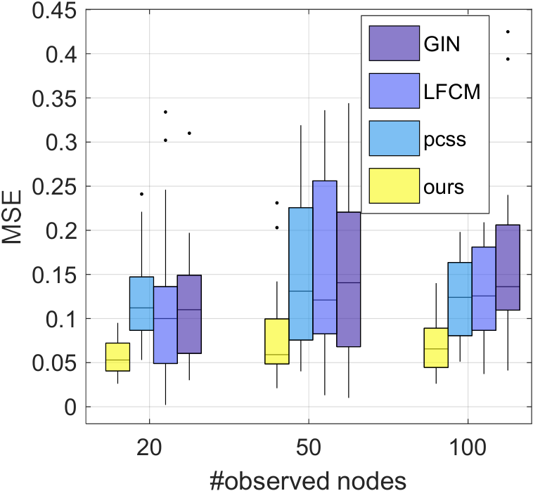
We are also concerned about the accuracy of the estimation of graph to justify our causal disentanglement, so we quantify the mean-squared estimation (MSE) error of . In Figure 5, our method likewise performs best in all ingredient settings, demonstrating that our confounding disentanglement pool the statistical strength better than other estimation algorithms in multi skeleton data. Besides, combined with the conclusion in [1], this error should decrease as the number of samples increases. Figure 5 (a) is exactly indicative of this conclusion. Additionally, to observe the distribution of graph and graph , we visualize the 2-D cluster of and in the varying of all ingredient settings. Appendix G.2 shows the projection of and extracted from the observation relation decoder and estimation function, respectively, using t-SNE [17]. The results indicate that our approach successfully disentangled the confounders and observed nodes through the true causal structure.
5.3 Real-World Data
| Modal | Method | Daily Dialog | MELD | EmoryNLP | IEMOCAP | RECCON |
| Text | Baseline | 54.31 | 60.91 | 34.42 | 65.22 | 63.51 |
| ACD | 55.47 | 59.47 | 35.18 | 65.13 | 65.29 | |
| CACD | 59.53 | 63.81 | 39.54 | 69.17 | 73.17 | |
| DAG-GNN | 57.19 | 61.48 | 38.22 | 67.85 | 71.36 | |
| biCD | 59.68 | 63.24 | 40.55 | 69.86 | 77.42 | |
| Video-Audio | Baseline | 58.30 | 56.49 | 51.87 | ||
| ACD | 58.67 | 63.27 | 68.26 | |||
| CACD | 60.18 | 68.47 | 70.83 | |||
| DAG-GNN | 61.22 | 66.83 | 73.21 | |||
| biCD | 64.62 | 69.47 | 76.59 |
To evaluate the quality of the deconfounding representation of that applies in further downstream tasks, we make the assessments in the real-world dataset of indefinite data. According to the endeavor of [5], affective reasoning tasks are adequate for investigating causal representation. The datasets are introduced in Appendix E.
In Table 2, ours has a much better representation ability than other models. Although ACD and CACD can recover causal representation from indefinite data, ACD only applies to the stationary confounders, and CACD is unable to deconfounding. Besides, it is interesting to observe that DAG-GNN lags further behind the ours. This performance differs from the synthetic definite data, indicating that the independent noise estimation is inadequate for indefinite data.
| Model | Datasets | ||||
|---|---|---|---|---|---|
| Daily Dialog | MELD | EmoryNLP | IEMOCAP | RECCON | |
| Ours | 59.68 | 63.24 | 40.55 | 69.86 | 77.42 |
| w/o | 1.12 | 2.11 | 0.85 | 3.09 | 2.29 |
| w/o | 1.57 | 1.58 | 1.64 | 2.33 | 3.74 |
| w/o estimation | 3.84 | 2.45 | 2.31 | 4.61 | 4.79 |
To validate the importance of each module in our method, in Table 3, we conduct ablation studies ‘w/o ’, ‘w/o ’, and ‘ w/o estimation’. is important for weighing confounding samples but removing it causes a performance decrease. Furthermore, sampling from adjacent matrix guarantees that our model can learn the invariance of multi-skeleton data, so removing also hampers the structure learning. Finally, ‘w/o ’ decreases most heavily, indicating that confounding disentanglement is crucial for recovering the true causal relations.
6 Discussion
| Causal Structure | Attribute | Edge |
|---|---|---|
| known () | known() | |
| substitute () | unknown | |
| partially known | unknown |
6.1 achievement of Our Method
Our method tries to recover entire causal relations including observed variables and latent confounders, while this appetite for indefinite data has been partially addressed.
Table 4 summarizes the achievement of our method in three causal structures. For , pure causal relations between observed variables, our method is capable of gaining attribute and edge. Our experiment also demonstrates that it does build a subgraph without confounding via as nodes and as edges. However, our method only gains esoteric knowledge for confounders via computing confounding effect . In other words, we do not know where and how many confounders are, which leads to the puzzle when we try to draw an edge from latent confounders to observed variables. Similarly, the unknown of latent confounders prevents us from understanding and computing the entire causal structures, thus hampering their construction.
This is also a prevalent obstacle existing in other causal discovery methods. Intrinsically, we can not obtain precise information on latent variables without any extra knowledge so we have to make many assumptions, set many conditions or find substitutes. Nevertheless, our endeavor of causal discovery in the presence of latent confounders has continued to show the feasibility of recovering entire relations from purely observational, non-experimental data.
6.2 Endogenous Confounders
Besides, another discussion is to explain the situation when latent confounders are not exogenous variables. Our model, especially two disentangled subgraphs, is based on an underlying assumption: each latent variable is exogenous, i.e., there is no edge like ‘’. So it is a problem of how our method works when there is an edge from an observed variable to a latent confounder.
In fact, our method achieve this problem by some projections as shown in Figure 6. We assume that , , , following the SCMs. In graph , we can obtain that:
| (31) | ||||
| (32) | ||||
| (33) |
In graph , we can obtain that:
| (35) | ||||
| (36) |
Overall, there is an underlying projection when our method handles these skeletons, which constructs an equal latent confounder to displace endogenetic and build direct edges from ancient observed nodes in the path when latent confounding is blocking.
7 Conclusion
In this paper, we first introduce two key traits- skeleton quantity and variable dimension, and three data paradigms of Causal Discovery. Then to learn the causal and deconfounding representation from indefinite data, we design a dynamic varaitional framework, which includes a deduction of the available variational posterior and analysis of dynamic reconstruction loss. The well-designed variational posterior settle down two essential problems induced by indefinite data (i.e., multi skeletons and multi values). Furthermore, the novel reconstruction describes the causal representation dynamic varying with the confounding effect’s strength. Moreover, we detailed comprehensive experiments on synthetic and real-world data to gauge the effectiveness of causal graph identification, causal disentanglement, and the high level performance of causal representation. Finally, we discuss the limitations about unknown information about causal graph and endogenous confounders. From the promising results, we thus argue that dynamic variational framework is our de facto need for causal discovery in an indefinite data paradigm.
References
- Agrawal et al. [2021] R. Agrawal, C. Squires, N. Prasad, and C. Uhler. The decamfounder: Non-linear causal discovery in the presence of hidden variables. arXiv preprint arXiv:2102.07921, 2021.
- Asuncion and Newman [2007] A. Asuncion and D. Newman. Uci machine learning repository, 2007.
- Bühlmann et al. [2014] P. Bühlmann, J. Peters, and J. Ernest. Cam: Causal additive models, high-dimensional order search and penalized regression. The Annals of Statistics, 42(6):2526–2556, 2014.
- Busso et al. [2008] C. Busso, M. Bulut, C.-C. Lee, A. Kazemzadeh, E. Mower, S. Kim, J. N. Chang, S. Lee, and S. S. Narayanan. Iemocap: Interactive emotional dyadic motion capture database. Language resources and evaluation, 42(4):335–359, 2008.
- Chen et al. [2023] H. Chen, J. Luo, X. Yang, and W. Zhu. Affective reasoning at utterance level in conversations: A causal discovery approach, 2023.
- Chickering [2002] D. M. Chickering. Optimal structure identification with greedy search. Journal of machine learning research, 3(Nov):507–554, 2002.
- Dhir and Lee [2020] A. Dhir and C. M. Lee. Integrating overlapping datasets using bivariate causal discovery. In Proceedings of the AAAI Conference on Artificial Intelligence, volume 34, pages 3781–3790, 2020.
- Dietrich et al. [2019] H. Dietrich, T. Wolf, T. Kawohl, J. Wehberg, G. Kändler, T. Mette, A. Röder, and J. Böhner. Temporal and spatial high-resolution climate data from 1961 to 2100 for the german national forest inventory (nfi). Annals of Forest Science, 76(1):1–14, 2019.
- Fan et al. [2022] S. Fan, X. Wang, Y. Mo, C. Shi, and J. Tang. Debiasing graph neural networks via learning disentangled causal substructure. arXiv preprint arXiv:2209.14107, 2022.
- Guvenir et al. [1997] H. Guvenir, B. Acar, G. Demiroz, and A. Cekin. A supervised machine learning algorithm for arrhythmia analysis. In Computers in Cardiology 1997, pages 433–436, 1997. doi: 10.1109/CIC.1997.647926.
- Herrett et al. [2015] E. Herrett, A. M. Gallagher, K. Bhaskaran, H. Forbes, R. Mathur, T. Van Staa, and L. Smeeth. Data resource profile: clinical practice research datalink (cprd). International journal of epidemiology, 44(3):827–836, 2015.
- Huang et al. [2019] B. Huang, K. Zhang, P. Xie, M. Gong, E. P. Xing, and C. Glymour. Specific and shared causal relation modeling and mechanism-based clustering. Advances in Neural Information Processing Systems, 32, 2019.
- Huang et al. [2020a] B. Huang, K. Zhang, M. Gong, and C. Glymour. Causal discovery from multiple data sets with non-identical variable sets. In Proceedings of the AAAI Conference on Artificial Intelligence, volume 34, pages 10153–10161, 2020a.
- Huang et al. [2020b] B. Huang, K. Zhang, J. Zhang, J. D. Ramsey, R. Sanchez-Romero, C. Glymour, and B. Schölkopf. Causal discovery from heterogeneous/nonstationary data. J. Mach. Learn. Res., 21(89):1–53, 2020b.
- Jiang and Veitch [2022] Y. Jiang and V. Veitch. Invariant and transportable representations for anti-causal domain shifts. arXiv preprint arXiv:2207.01603, 2022.
- Kingma and Welling [2022] D. P. Kingma and M. Welling. Auto-encoding variational bayes, 2022.
- Knyazev et al. [2019] B. Knyazev, G. W. Taylor, and M. Amer. Understanding attention and generalization in graph neural networks. Advances in neural information processing systems, 32, 2019.
- Li et al. [2017] Y. Li, H. Su, X. Shen, W. Li, Z. Cao, and S. Niu. DailyDialog: A manually labelled multi-turn dialogue dataset. In Proceedings of the Eighth International Joint Conference on Natural Language Processing (Volume 1: Long Papers), pages 986–995, Taipei, Taiwan, Nov. 2017. Asian Federation of Natural Language Processing. URL https://aclanthology.org/I17-1099.
- Löwe et al. [2022] S. Löwe, D. Madras, R. Zemel, and M. Welling. Amortized causal discovery: Learning to infer causal graphs from time-series data. In Conference on Causal Learning and Reasoning, pages 509–525. PMLR, 2022.
- Lv et al. [2022] F. Lv, J. Liang, S. Li, B. Zang, C. H. Liu, Z. Wang, and D. Liu. Causality inspired representation learning for domain generalization. In Proceedings of the IEEE/CVF Conference on Computer Vision and Pattern Recognition, pages 8046–8056, 2022.
- Maddison et al. [2016] C. J. Maddison, A. Mnih, and Y. W. Teh. The concrete distribution: A continuous relaxation of discrete random variables. arXiv preprint arXiv:1611.00712, 2016.
- Oh et al. [2021] G. Oh, E. Jeong, and S. Lim. Causal affect prediction model using a facial image sequence. arXiv preprint arXiv:2107.03886, 2021.
- Poria et al. [2019] S. Poria, D. Hazarika, N. Majumder, G. Naik, E. Cambria, and R. Mihalcea. MELD: A multimodal multi-party dataset for emotion recognition in conversations. In Proceedings of the 57th Annual Meeting of the Association for Computational Linguistics, pages 527–536, Florence, Italy, July 2019. Association for Computational Linguistics. doi: 10.18653/v1/P19-1050. URL https://aclanthology.org/P19-1050.
- Poria et al. [2021] S. Poria, N. Majumder, D. Hazarika, D. Ghosal, R. Bhardwaj, S. Y. B. Jian, P. Hong, R. Ghosh, A. Roy, N. Chhaya, et al. Recognizing emotion cause in conversations. Cognitive Computation, 13(5):1317–1332, 2021.
- Schölkopf et al. [2021] B. Schölkopf, F. Locatello, S. Bauer, N. R. Ke, N. Kalchbrenner, A. Goyal, and Y. Bengio. Toward causal representation learning. Proceedings of the IEEE, 109(5):612–634, 2021.
- Shen et al. [2021] W. Shen, S. Wu, Y. Yang, and X. Quan. Directed acyclic graph network for conversational emotion recognition. In Proceedings of the 59th Annual Meeting of the Association for Computational Linguistics and the 11th International Joint Conference on Natural Language Processing (Volume 1: Long Papers), pages 1551–1560, Online, Aug. 2021. Association for Computational Linguistics. doi: 10.18653/v1/2021.acl-long.123. URL https://aclanthology.org/2021.acl-long.123.
- Shimizu and Bollen [2014] S. Shimizu and K. Bollen. Bayesian estimation of causal direction in acyclic structural equation models with individual-specific confounder variables and non-gaussian distributions. J. Mach. Learn. Res., 15(1):2629–2652, 2014.
- Shimizu et al. [2006] S. Shimizu, P. O. Hoyer, A. Hyvärinen, A. Kerminen, and M. Jordan. A linear non-gaussian acyclic model for causal discovery. Journal of Machine Learning Research, 7(10), 2006.
- Smith et al. [2011] S. M. Smith, K. L. Miller, G. Salimi-Khorshidi, M. Webster, C. F. Beckmann, T. E. Nichols, J. D. Ramsey, and M. W. Woolrich. Network modelling methods for fmri. Neuroimage, 54(2):875–891, 2011.
- Spirtes et al. [2000] P. Spirtes, C. N. Glymour, R. Scheines, and D. Heckerman. Causation, prediction, and search. MIT press, 2000.
- Squires et al. [2022] C. Squires, A. Yun, E. Nichani, R. Agrawal, and C. Uhler. Causal structure discovery between clusters of nodes induced by latent factors. In Conference on Causal Learning and Reasoning, pages 669–687. PMLR, 2022.
- Veličković et al. [2017] P. Veličković, G. Cucurull, A. Casanova, A. Romero, P. Lio, and Y. Bengio. Graph attention networks. arXiv preprint arXiv:1710.10903, 2017.
- Verma and Pearl [1992] T. Verma and J. Pearl. An algorithm for deciding if a set of observed independencies has a causal explanation. In Uncertainty in artificial intelligence, pages 323–330. Elsevier, 1992.
- Wang et al. [2020] Y. Wang, V. Menkovski, H. Wang, X. Du, and M. Pechenizkiy. Causal discovery from incomplete data: a deep learning approach. arXiv preprint arXiv:2001.05343, 2020.
- Wu et al. [2022] Y.-X. Wu, X. Wang, A. Zhang, X. He, and T.-S. Chua. Discovering invariant rationales for graph neural networks. arXiv preprint arXiv:2201.12872, 2022.
- Xie et al. [2020] F. Xie, R. Cai, B. Huang, C. Glymour, Z. Hao, and K. Zhang. Generalized independent noise condition for estimating latent variable causal graphs. Advances in Neural Information Processing Systems, 33:14891–14902, 2020.
- Yu et al. [2019] Y. Yu, J. Chen, T. Gao, and M. Yu. Dag-gnn: Dag structure learning with graph neural networks. In International Conference on Machine Learning, pages 7154–7163. PMLR, 2019.
- Zahiri and Choi [2018] S. Zahiri and J. D. Choi. Emotion Detection on TV Show Transcripts with Sequence-based Convolutional Neural Networks. In Proceedings of the AAAI Workshop on Affective Content Analysis, AFFCON’18, pages 44–51, New Orleans, LA, 2018. URL https://sites.google.com/view/affcon18.
- Zhao et al. [2022] W. Zhao, Y. Zhao, Z. Li, and B. Qin. Knowledge-bridged causal interaction network for causal emotion entailment. arXiv preprint arXiv:2212.02995, 2022.
- Zheng et al. [2018] X. Zheng, B. Aragam, P. K. Ravikumar, and E. P. Xing. Dags with no tears: Continuous optimization for structure learning. Advances in neural information processing systems, 31, 2018.
.1 Structural Causal Model (SCM)
The causal additive model (CAM) has some desirable properties, making it a suitable method for introducing low-dimensional structures to improve statistical efficiency and flexibility [3, 27]. To attempt to unveil the causal structure of indefinite data, we will first provide an interpretation of SCMs in indefinite data. We begin with a general CAM for definite data, assuming that any node in definite data satisfies the following generating process:
| (38) |
where represents the independent and identically distributed noise variable (Existing methods support it satisfies some particular distribution assumption, including both non-gaussian distribution [28] or gaussian distribution [1]). represents the causal strength from node to in -th sample. is the parent set of . Without loss of generality, we can omit the sample number . Continuing equation 38, we make CAM assumption for indefinite data and consider the following generating process:
| (39) |
where is a distribution-agnostic noise variable. represents the -th multi-value node in -th skeleton. Consequently, we can obtain the general definition of SCM between any sample in definite data and any sample in one skeleton of indefinite data:
Definition 4 (Structural Causal Model).
An SCM is a 3-tuple , where is the entire set of observed variables . Structural equations are functions that determine with , where . is a distribution over .
Appendix A Proof of Definition 3
By equation 7 in main text and 39 in Appendix,
| (40) |
Hence,
| (41) | ||||
| (42) |
Intuitively, the term reflects a particular graph consisting of . Hence, we would like to transform Equation 42 into a statistic about ‘’. Fortunately, a sufficient statistic is supported by [1]. It makes identifiable under the Gaussian and . Along with their inference, we find the branch point under our data condition:
| (43) | ||||
| (44) |
If the is negligible, we can obtain the same statistic due to . In other words, when apparently exceeds , latent confounders essentially contribute the , and naturally, is meaningless when it is mainly affected by .
Finally, we could approximately estimate the discrete probability of under a strong confounding assumption:
| (46) | ||||
| (47) |
Additionally, is not easy to calculate under weak confounding, so the dynamic reconstruction loss function does not consider C when confounding influence is insufficient (See Subsection “Dynamic Reconstruction Error” for details).
Appendix B Datasets
Synthetic datasets afford several advantages not present in real-world datasets. For instance, causal relationships within synthetic datasets remain unbiased; synthetic datasets grant control over the sample size of each structure within the multi-skeleton setting. In addition, complete labels for latent confounding can be included in synthetic datasets; along with the capacity to dictate variations in other parameters, such as the quantity of observed nodes and confounders. However, synthetic datasets also exhibit certain limitations, primarily their inability to construct multi-value variables. This arises due to the complex interdependencies between values within these variables, which cannot be defined through distribution assumptions.
Therefore, to conduct the proposed experiment, we adopt an approach incorporating both synthetic and real-world datasets. The synthetic datasets function as semi-definite data involving multi-skeleton and single-value data. This setup seeks to evaluate the causal discovery capabilities of our proposed methods and their ability to decouple confoundings under various conditions under multi skeletons. The real-world datasets, composed of indefinite data with multi-skeleotn and multi-value, aim to measure the actual enhancement provided by our model-generated causal representations for high-level tasks. Table 5 shows the detailed statistic about synthetic datasets and real-word datasets.
B.1 Synthetic Data
| Category | Dataset | Train Set | Valid Set | Test Set | |||
|---|---|---|---|---|---|---|---|
| sample | skeleton | sample | skeleton | sample | skeleton | ||
| Synthetic | Syn1 | 2250 | 450 | 500 | 100 | 1000 | 200 |
| Syn2 | 4500 | 450 | 1000 | 100 | 2000 | 200 | |
| Syn3 | 22500 | 450 | 5000 | 100 | 10000 | 200 | |
| Syn4-9 | 22500 | 450 | 5000 | 100 | 10000 | 200 | |
| Real-world | DailyDialog | 11118 | 35 | 1000 | 25 | 1000 | 23 |
| MELD | 1038 | 14 | 114 | 7 | 280 | 9 | |
| EmoryNLP | 713 | 31 | 99 | 14 | 85 | 11 | |
| IEMOCAP | 100 | 13 | 20 | 4 | 31 | 5 | |
| RECCON-DD | 833 | 37 | 47 | 15 | 225 | 28 | |
| RECCON-IE | 16 | 14 | |||||
| ID | sample | confounder | observed nodes | pervasiveness |
|---|---|---|---|---|
| Syn1 | 5 | 1 | 50 | 0.7 |
| Syn2 | 10 | 1 | 50 | 0.7 |
| Syn3 | 50 | 1 | 50 | 0.7 |
| Syn4 | 50 | 5 | 50 | 0.7 |
| Syn5 | 50 | 10 | 50 | 0.7 |
| Syn6 | 50 | 1 | 20 | 0.7 |
| Syn7 | 50 | 1 | 100 | 0.7 |
| Syn8 | 50 | 1 | 50 | 0.1 |
| Syn9 | 50 | 1 | 50 | 0.4 |
Specifically, We randomly draw Causal DAG from a random graph model with an expected neighborhood size of 5 and consider graphs with the number of observed nodes . For probing how our approach is affected by the pervasiveness of confounding, we assume that each confounder is a direct cause of node with a chance . Given the graph, we stochastically set a trend type for each causal strength weight with equal probability. Meanwhile, we add noise to each node. Finally, we consider the number of confounders and the number of samples of each skeleton , respectively. These key ingredients of each set of synthetic data are shown in Table 6.
B.2 Real-World Data
We use five real datasets for two affective reasoning tasks. These datasets are conducted by Conversational Affective Causal Discovery (CACD) [5].
DailyDialog [18]: A Human-written dialogs dataset with 7 emotion labels (neutral, happiness, surprise, sadness, anger, disgust, and fear). We follow [26] to regard utterance turns as the speaker turns.
MELD [23]: A multimodel ERC dataset with 7 emotion labels as the same as DailyDialog.
EmoryNLP [38]: A TV show scripts dataset with 7 emotion labels (neutral, sad, mad, scared, powerful, peaceful, joyful).
IEMOCAP [4]: A multimodel ERC dataset with 9 emotion labels (neutral, happy, sad, angry, frustrated, excited, surprised, disappointed, and fear). However, models in ERC field are often evaluated on samples with the first six emotions due to the too few samples of the latter three emotions. 20 dialogues for validation set is following [26].
RECCON [24]: The first dataset for emotion cause recognition of conversation including RECCON-DD and RECCON-IE (emulating an out-of-distribution generalization test). RECCON-DD includes 5380 labeled ECPs and 5 cause spans (no-context, inter-personal, self-contagion, hybrid, and latent).
Appendix C Baselines and Experiment setup
To the best of our knowledge, no baseline approach is broadly applicable in single-value and multi-value data, even single-skeleton and multi-skeleton datasets. So we choose the SOTA work in Causal Discovery from definite and indefinite data, respectively. In synthetic data, we investigated pcss [1], LFCM [31], and GIN [36], which are all SOTA approaches in Causal Discovery, especially from single-value and single-skeleton data.
pcss: estimates causal relationships in the non-linear, pervasive confounding setting by leveraging an approximate spectral decomposition of the observed data matrix.
LFCM: finds ordered clusters of observed nodes, a partial ordering over clusters, and finally the entire structure over both observed and latent nodes via the theorem of Trek separation and Tetrad representation.
GIN: designs a Linear Non-Gaussian Latent variable Model to identify important information, including where the latent variables are, the number of latent variables behind any two observed variables, and the causal order of the latent variables.
In Real-world data, we investigated DAG-GNN [37], ACD [19] and CACD [5]. DAG-GNN is the SOTA method for single-skeleton and multi-value data, ACD is the SOTA method for multi-skeleton data while single-value. CACD is the SOTA work on multi-skeleton and multi-value data while neglecting the confounding.
ACD: leverages shared dynamics to learn to infer causal relationships from multi-skeleton time-series data via a single, amortized model.
CACD: discover causal relationships in multi-value data via designing a common skeleton and generating a substitute for independent noise.
DAG-GNN: leverages SEM to construct a gnn-based variational model adopting independent noise as latent viariable.
Due to dissatisfing data structure, ACD and CACD are not capable for synthetic data. In synthetic data, we only add DAG-GNN to represent indefinite data method. Besides, pcss, LFCM, and GIN are all unavailable for real-world dataset.
Appendix D Visualization
D.1 Causal Strength
In Figure 7, we illustrate the causal graph generated by various methods, based on samples of 20 observed variables, in the form of adjacency matrices. For each in the matrix, the value signifies the probability of a causal relationship from node to (); therefore, the graph is a strict lower-triangular matrix. Subfigure f represents the actual causal model, w hile subfigure a-e display the predictions made by various methods concerning this causal structure. Significant similarities are observed between our approach (subfigure e) and ground truth f, as evidenced by the highest number of correct predictions (and the least number of incorrect predictions) attained via our method: On average, for a causal structure with 20 observational nodes, our method exceeds other approaches by predicting over 2 directed edges correctly and lessens the error by over 1 predicted directed edge. However, this is an unsuitable metric, as it does not consider the continuous values of the causal relationships. Consequently, we utilize the AUROC for the quantitative experimentation.


D.2 2-D Cluster Visualization


