Task-Aware Risk Estimation of
Perception Failures for Autonomous VehiclesManuscript received January 20, 2002; revised August 13, 2002.
Abstract
Safety and performance are key enablers for autonomous driving: on the one hand we want our autonomous vehicles (AVs) to be safe, while at the same time their performance (e.g., comfort or progression) is key to adoption. To effectively walk the tight-rope between safety and performance, AVs need to be risk-averse, but not entirely risk-avoidant. To facilitate safe-yet-performant driving, in this paper, we develop a task-aware risk estimator that assesses the risk a perception failure poses to the AV’s motion plan. If the failure has no bearing on the safety of the AV’s motion plan, then regardless of how egregious the perception failure is, our task-aware risk estimator considers the failure to have a low risk; on the other hand, if a seemingly benign perception failure severely impacts the motion plan, then our estimator considers it to have a high risk. In this paper, we propose a task-aware risk estimator to decide whether a safety maneuver needs to be triggered. To estimate the task-aware risk, first, we leverage the perception failure —detected by a perception monitor— to synthesize an alternative plausible model for the vehicle’s surroundings. The risk due to the perception failure is then formalized as the “relative” risk to the AV’s motion plan between the perceived and the alternative plausible scenario. We employ a statistical tool called copula, which models tail dependencies between distributions, to estimate this risk. The theoretical properties of the copula allow us to compute probably approximately correct (PAC) estimates of the risk. We evaluate our task-aware risk estimator using NuPlan and compare it with established baselines, showing that the proposed risk estimator achieves the best -score (doubling the score of the best baseline) and exhibits a good balance between recall and precision, i.e., a good balance of safety and performance.
I Introduction
Despite the fast-paced progress in robotics and autonomous systems, perception modules in autonomous vehicles (AVs) still encounter a spate of failure modes (e.g., misclassification or misdetection of objects, ghost obstacles, out-of-distribution (OOD) objects, etc.), which can compromise the safety of passengers, other drivers, and pedestrians. Consequently, the problem of developing detectors for such perception failures has recently gained traction [4, 44, 35, 10]. However, these failures occur frequently enough that reverting to a fallback safety maneuver for each such detection is prohibitively detrimental to the performance of the AV. In this paper, we work towards developing a task-aware perception monitor that only triggers when the perception failure poses a significant risk to the AV’s motion plan, thereby, promoting safe yet performant driving; an example highlighting the importance of developing a task-aware perception monitor, which focuses on task-relevant perception failures, is illustrated in Fig. 1.
We envision a task-aware perception monitor that embodies three main components, as shown in Fig. 2. First, the perception failure detection and identification module identifies perception faults and isolates the responsible modules and failure modes. Second, the plausible scene generator leverages the knowledge of the perception failure modes, provided by the failure identification, to construct a probabilistic (possibly multi-modal) description of plausible alternative models for the AV’s surroundings that supports the actual world scene.11 1 The probabilistic description of plausible AV surroundings might be highly stochastic and multi-modal. Planning in the plausible scene would be impractical and possibly not conducive to a good plan; however, we can still leverage it to estimate the risk of the perception failures to the AV using the approach we develop in this paper. Finally, a task-aware risk estimator assesses the increased risk to the AV’s motion plan due to the perception failure. There is a plethora of recent work on perception failure detection [4, 40, 35, 10], and also some work on plausible scene generation [11, 24, 3], comparably much less work on task-aware risk estimation. The primary subject of this paper is, indeed, the development of the task-aware risk estimator.
The task-aware risk estimator we develop in this paper compares the risk to the AV’s motion plan in the perceived scenario with the one in the generated plausible scenarios. The risk posed to the AV’s motion plan in both the scenes (perceived and plausible) is expressed as a probability distribution on a risk metric, e.g., time-to-collision. We introduce the notion of relative scenario risk (RSR), which measures the probability that the plausible scene has a high risk when the perceived scene does not. To empirically estimate RSR, we employ the statistical tool called copula [38], which models tail dependencies between distributions, and we provide probably approximately correct (PAC) bounds on the RSR estimate. Finally, we provide a detection algorithm based on the RSR PAC bounds that, with high probability, triggers an alarm when faced with high-risk task-relevant failures.
Statement of Contributions. Our contributions in this paper are as follows: (i) We formalize the notion of relative scenario risk (RSR), which underlies our task-aware risk estimation; (ii) We develop an algorithm to estimate RSR at runtime by leveraging the copula and also provide probabilistic guarantees on the correctness of our estimation; (iii) Finally, we demonstrate the efficacy of our framework by comparing our method with prior approaches on a dataset of realistic perception failure scenarios created in NuPlan [18]. We show that our risk estimator achieves the highest F1 score, exhibits a good balance of precision and recall, and anticipates collisions with sufficient time to allow mitigation measures. The code is available at https://github.com/NVlabs/persevere.
II Related Work
We discuss prior art for all of the three stages of our perception monitoring scheme, i.e., perception failure detection, plausible scene generation, and task-relevant risk estimation.
Perception Failure Detection and Identification. Autonomous vehicles rely on onboard perception systems to provide situational awareness and inform the onboard decision-making and control systems. Reliability of the perception system is critical for safe operation of AVs. While it is desirable for the perception system to be fault-free under any conditions, it is hard to guarantee it [10]; therefore, detection and identification of failures in the perception system at runtime have gained increasing attention. The problem of fault detection and identification is studied in [3] where the authors proposed a system-level framework for online monitoring of the perception system of an AV. Besides failure detection, the framework in [3] also identifies, at runtime, the failure modes that the system is experiencing, from an a priori known list of failures. Other approaches in the literature include spatio-temporal information from motion prediction to assess 3D object detection [47], Timed Quality Temporal Logic (TQTL) to reason about desirable spatio-temporal properties of a perception algorithm [5, 6], or detect anomalies by placing logical-constraint model assertions [28]. Since perception systems are composed of multiple modules, failure detection for specific submodules has also received attention. Previous works focused on object detection [35], semantic segmentation [9, 39], localization [25, 19], out-of-distribution (OOD) detection [42, 21], or changes in high-definition map [30]. All of the above works focus on detecting and identifying failures in the perception system, but do not assess their impact on the AV’s motion plan.
Plausible Scene Generation. While there is limited prior work on explicit plausible scene generation, many works in the literature reason about plausible alternative scenes in order to detect or avoid failures. Indeed, failure detection methods often use spatio-temporal inconsistencies between different sensor modalities, where each modality implicitly proposes a plausible scene. You et al. [47] use historical information from a number of previous 3D scenes to predict a plausible scene, that is then compared with the perceived scene to detect errors. Similarly, [33] correlates camera images and LIDAR point clouds to detect missing (or ghost) obstacles. Beside obstacle detection, previous work also tackled the mislocalization error. Li et al. [32] use particle filters to retain multiple likely positions of the AV. Futhermore, the literature on planning under occlusions contains both model-based [17, 29, 48] and learning based approaches [11, 24, 20]. These works augment the scene to include possible missing (occluded) obstacles in the scene. The same techniques can be used to generate plausible scenes whenever the failure detection does not provide enough information about the plausible scene.
Risk Assessment. There are several risk assessment techniques in the literature [12, 46]. One approach to “measure” the risk is to monitor the deterioration of the cost of the motion plan, as was done in [15, 14, 16]. Another approach is to use a criticality metric, such as Time To Collision (TTC), which computes the time before a collision happens between two actors if their speeds and orientations remain the same. There is a large variety of criticality metrics in the literature, and the interested reader is referred to [46] for a comprehensive overview; however, these metrics, in general, only assess whether a scenario is dangerous while assuming that the inferred scene from perception is correct. A recent approach uses a neural network to classify the risk level using labeled data [1]. However, learning-based methods suffer from lack of OOD robustness, and are usually less interpretable and lack guarantees. Other works on perception-aware risk assessment, such as [7], which proposes risk-ranked recall for object detection systems, and [8], which develops perception-uncertainty-based risk envelopes, do not reason about the future actions of other agents. Topan et al. [44] do account for the future actions of other agents for perception failures by computing “inevitable” collision sets (ICS) via Hamilton-Jacobi (HJ) reachability analysis [36], and flagging a situation as unsafe if another agent is close to entering the ICS [31, 22, 23]. However, [44] assumes the worst-case scenario will occur, i.e., the AV and other road agents will try to collide with each other, and does not consider the interactions between multiple agents, resulting in over-conservatism. In this paper, we estimate the risk to the AV’s motion plan in the presence of a perception failure while accounting for future actions of other agents by leveraging a trajectory prediction network [41]. Furthermore, our approach is accompanied with PAC bounds and is run-time capable.
III Task-Aware Perception Monitors: Overview and Risk Estimation Formulation
This section provides an overview of the building blocks of our task-aware perception monitor, which comprises of three components: perception failure detection and identification, plausible scene generator, and task-aware risk estimator. Moreover, the section formalizes the problem of task-aware risk estimation, which is the main focus of this paper. Throughout the rest of the paper we will refer to the AV as the ego vehicle while any other agent is referred to as a non-ego agent.
Perception Failure Detection and Identification. We assume access to a perception failure detection and identification module, such as the algorithms presented in [3], that identifies the set of failure modes the perception system is experiencing. The perception system is composed of a set of modules, each of which is responsible for a specific task, e.g., object detection, localization, etc. Each module is subject to a finite set of failure modes. The perception failure detection and identification module computes a failure state vector , containing the relevant information about the active failures, that is, the set of active failure modes and the corresponding perception diagnostic information (such as intermediate detection results, raw sensor data, etc.).
Plausible Scene Generator. Before we assess the risk that the perception failure poses to the AV’s motion plan, we need to understand the actual scene in which the AV is operating. To this end, we construct a new estimate of the surrounding scene using what we call a plausible scene generator . Let be an estimate of the world state at time , provided by the perception module (this is the “perceived scene”). We assume that the world state comprises the ego vehicle’s state , non-ego agents’ states , and map attributes , e.g., lane lines, stop signs, traffic signals, etc. Given the perceived world state from the perception module, and the active perception failure modes information from the perception failure detection and identification, the plausible scene generator returns alternative plausible scenes in the form of a probability distribution over the plausible world states at time ; we require the plausible scene generator to support the actual world state.
While there are some approaches that can be used for scenario generation [3, 47, 11, 24, 20], the approach we adopt here is based on the perception failure identification method in [3]. In a nutshell, the method in [3] detects inconsistencies between intermediate perception results and infers the set of faults that could have caused such inconsistencies.22 2 The method [3] can also integrate more complex tests, including logic formulas, mathematical certificates of correctness, and a priori bounds. For instance, consider the case where the radar-based detection module detects an obstacle in front of the ego-vehicle, but the same obstacle is missed by the camera-based detection module: in this case the perception system might prioritize camera detection and discard the radar detection as a false detection; therefore, the perceived scene would have no obstacle in front of the ego-vehicle. However, the approach in [3] can detect the inconsistency between the radar and the camera and, making spatio-temporal considerations, can infer that the radar detection is indeed correct. The plausible scene generator can then use the information about the failure to generate an alternative plausible scene that contains an obstacle as detected by the radar. In general, the alternative scene may not be unique. For example, since the radar-based detection module may only be able to detect the position and the velocity of the missing obstacle, but not its class (e.g., car, pedestrian, etc.), such a detected failure may give rise to a probability distribution over plausible scenes (e.g., the uniform distribution over the missing obstacle’s class). Similarly, this distribution can also model uncertainty in the radar position and velocity measurements. Assuming that at least a module in the perception pipeline computed the correct result, the distribution of generated scenes will support the actual scene.33 3 This approach can also be generalized to early-fusion and middle-fusion perception systems as spatio-temporal information across frames can provide useful diagnostic information regardless of the perception architecture. In this paper, we do not assume a particular implementation of the plausible scene generator, which might depend on the perception system architecture, but we rather focus on the risk assessment. We only require the plausible scene distribution to support the actual scene, which has been shown to be possible for the most common perception failure modes [3, 47, 11, 33, 17] (as discussed in Section II).
Relative Scenario Risk. We are interested in understanding how much more risk does the ego’s motion plan encounter in the generated plausible scenes compared to the perceived scene . Let be the ego’s motion plan generated by a planning module for a time horizon . We assume the availability of a trajectory prediction module which provides a distribution on the future world state trajectories conditioned on the world state history and the ego’s motion plan. The trajectory predictor reasons about agent interactions and provides multimodal predictions that account for multiple agent intentions; in our experiments we use Trajectron++ [41] which is a state-of-the-art trajectory prediction model that satisfies these criteria. The approach we describe is agnostic to the choice of the planning and prediction modules. Let be a cost function such that higher values imply riskier scenarios for the ego vehicle. Examples of such functions might be the distance between the ego vehicle and the closest non-ego agent or a surrogate (so that higher values imply smaller times) of the time-to-collision metric [46]. The distribution on the future world states induces a sequence of univariate distributions over the predicted costs for each time step in the future. In the rest of the paper, we will work with the predicted cost distribution for a particular and for a particular motion plan . For the sake of notational compactness, we drop the explicit dependence of on and to express the predicted cost distribution as . Similarly, the plausible scene distribution on the plausible world state induces the cost distribution .
We are now ready to formalize our task-aware notion of risk in the following definition.
Definition 1 (Relative Scenario Risk (RSR)).
Let be the world state history for the perceived scene and let be the distribution of the generated plausible scenes due to the perception faults , detected by a perception failure detection and identification module. Let be the distribution of the costs for the perceived scene and be the distribution of the costs for the plausible scenes. Let be the cost threshold that the planner desires to stay below. The relative scenario risk (RSR) between the plausible and the perceived scenes is then defined as:
| (1) |
For a given , the higher the RSR is, the further the plausible scene cost distribution is skewed towards higher costs, as illustrated in Fig. 2. Hence larger values of imply that the plausible scenes are riskier than the perceived scene. Note that, in the general, and will not be independent as the underlying scene is largely the same.
The choice of defines a desired safety threshold: for instance, if the cost is the distance between agents, can be the smallest acceptable distance between the ego and the nearest agent. The choice of may be scenario dependent (e.g., the minimum distance might be different when driving on a highway vs. a traffic jam). To overcome this dependency, we take to capture the bulk of the probability mass in the perceived scene cost distribution (). To make this more concrete, let be the marginal cumulative distribution function (CDF) of and be the CDF of . Recall that the generalized inverse of a CDF , here denoted by , is defined as:
| (2) |
Then, we choose . This is equivalent to taking to be the maximum value of the risk cost, among the most common situations in the perceived scene. We call the risk aversion parameter as it denotes the amount of risk the ego agent is willing to accept in its motion plan.
We can now define the -quantile relative scenario risk.
Definition 2 (-quantile Relative Scenario Risk).
Let be the relative scenario risk in Definition 1. Let be the risk aversion parameter described above. Then, the -quantile relative scenario risk (-RSR) is defined as:
| (3) |
Note that the definition above is simply restating Definition 1 in terms of the risk aversion parameter .
Problem Statement. Given the perceived world state history , the perception module fault modes , and risk aversion , we want to estimate the -quantile relative scenario risk in Definition 2. It is worth pointing out that this is a challenging problem because the distributions and are not independent, and we do not have an explicit analytical representation for them or their CDFs , ; hence, we cannot analytically compute or . However, we can sample from these distributions independently. In particular, we take samples from these distributions in a way that they are independent (any new sample does not depend on the previous) and identically distributed (the underlying scene and behavior of the agents is fixed). In the next section, we present a method to estimate using these samples.
IV Task-Aware Risk Estimation
In this section, we use copulas [26], a statistical tool used to model tail dependencies between distributions, to provide an algorithm to estimate the RSR defined in Definition 2.
IV-A Introduction to Copulas
To model the dependency between the two univariate distributions and , we use the concept of copula (for a more extensive introduction see [26, Chapter 1]). Copulas are tools for modelling dependence of several random variables, and the name “copula” was chosen to emphasize the manner in which a copula couples a joint distribution function to its univariate marginals. We make this mathematically precise in the following definition.
Definition 3 (Copula [38]).
A -dimensional copula is a function defined on a -dimensional unit cube that satisfies the following:
- 1.
for any , ,
- 2.
for any in any position, and
- 3.
is -non-decreasing.44 4 That is, for each hyper-rectangle , the C-volume of is non-negative: , where
These three properties ensure that the copula behaves like a joint distribution function. To gain intuition, consider each to be a probability in the range . The first condition says that if the probability of the event associated to is zero, then, regardless of the probability of the other events, the joint probability of all events happening at the same time is zero. Conversely, if all events are sure to occur except one, then the probability of the joint event is the probability of the single non-sure event. Finally, the last condition imposes the copula to be non-decreasing in each component.
Sklar’s theorem [43], presented next, provides the theoretical foundation for the application of copulas together with the conditions for the existence (and uniqueness) of the copula. Note that in this paper, we only require the existence of the copula, but we include the uniqueness conditions as well below for the sake of completeness.
Theorem 1 (Sklar’s theorem [43]).
Let be a joint distribution function, and let , be the marginal distributions. Then, there exists a copula such that for all in
| (4) |
Moreover, if the marginals are continuous, then is unique; otherwise, is uniquely determined on where denotes the range (image) of .
The importance of copulas in studying multivariate distribution is emphasized by Sklar’s theorem, which shows, firstly, that all multivariate distribution can be expressed in terms of copulas, and secondly, that copulas may be used to construct multivariate distribution functions from univariate ones. The latter point is particularly important for us because, as we noted in the previous section, we cannot sample from the joint distribution , but we can sample from the marginals and .
IV-B Estimating -RSR using Copula
Let , be random variables drawn from and with CDFs and , respectively (notation introduced in Definition 1); as a quick reminder, is the cost distribution of the perceived scene and of the plausible scene. Let’s assume for a moment that we can estimate the copula relating and . Since the copula contains the information on the dependence structure between , we can use it to measure the tail dependency between the two distributions. Hence, using the definition of conditional probability and Eq. 4 from Theorem 1, we can express -RSR in Eq. 1 as follows:55 5 For notational brevity, we are dropping the distributions from which the random variables and are drawn from under the probability sign .
| (5) | ||||
Unfortunately, we do not have access to the explicit expression of the two CDFs and and the copula , therefore, cannot be computed analytically. In what follows, we will provably bound by constructing empirical estimates and of the CDFs and , respectively, with i.i.d. samples from both, and .
Theorem 2 (PAC bound on -RSR).
Let and be i.i.d. samples from CDFs and , respectively. Let
be empirical estimates of and , respectively. Let the risk aversion parameter be as described in Section III and let . Then, with probability at least :
where
and .
Proof.
See Section -A. ∎
Both bounds are sharp in the sense that they can be attained. In particular, the lower bound is attained when and are perfectly positively dependent in the sense that is almost surely a strictly increasing function of . Conversely, the upper bound is attained when and are perfectly negatively dependent, meaning that is almost surely a strictly decreasing function of .
The PAC bounds in Theorem 2 are tractable to compute and allow us to estimate -RSR at runtime. In particular the assumption on i.i.d. samples is not restrictive: as we noted in Section III, our problem formulation allows i.i.d. samples. Also we do not assume a particular copula, but only its existence, which is proved by Sklar’s theorem.
IV-C Triggering Safety Maneuvers
With the results presented in Theorem 2, we have a way to measure if, compared to the perceived scene, the plausible scene exposes the ego-vehicle to unwanted risk in terms of probability. However, if the probability is low, it might be detrimental for the ego-vehicle’s performance to trigger safety maneuvers to mitigate the risk. In the following we design a detection algorithm (Algorithm 1) that can be used to detect if the system is likely to be experiencing a high-risk situation, which can be used to trigger safety maneuvers.
Consider a risk threshold that denotes high-risk situations. If the lower bound on in Theorem 2 is above , it means that with probability at least , the current scene indeed corresponds to a high-risk situation (in the sense of -RSR). In such a case, Algorithm 1 detects a task-relevant failure (line 7), which can be used to trigger a safety maneuver. This reasoning can be easily extended to consider multiple thresholds for multiple criticality levels, each associated with different mitigation strategies or different driving scenarios (e.g., highway, urban driving, pickup/drop-off, etc.).
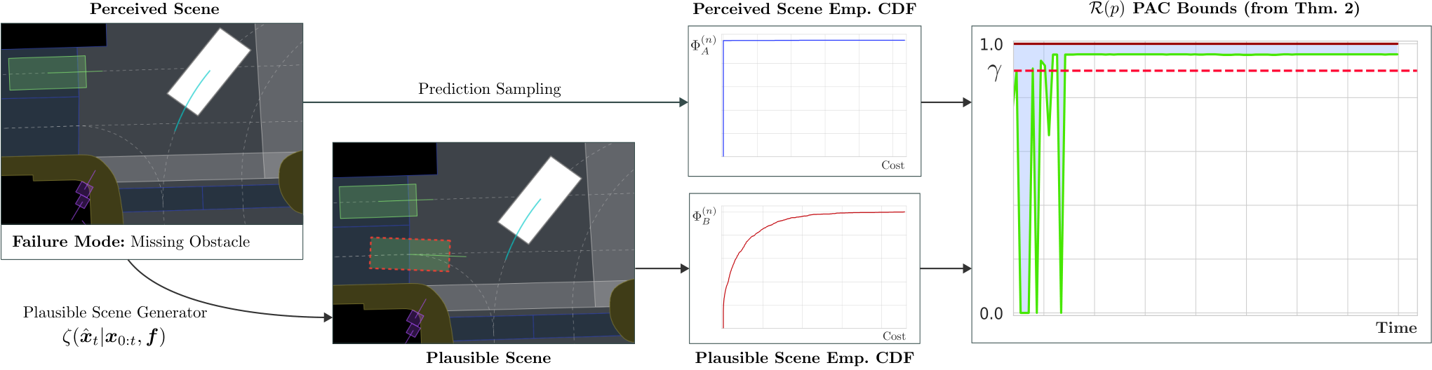
Algorithm 1 can be summarized as follows: after a failure is identified and the plausible scene generated, the algorithm samples the two scenes (line 3) and estimates the empirical CDFs (lines 4-5). It then returns if the lower bound in Theorem 2 is above the risk threshold , or otherwise (line 6). The algorithm steps are depicted in Fig. 3.
The algorithm has four parameters: the risk aversion , the risk threshold , the number of samples , and the confidence level . The risk aversion measures the risk tolerance of the ego-vehicle, in terms of quantiles of the perceived scene risk distribution. Higher values indicate high risk tolerance, i.e., the ego-vehicle is be expected to behave safely in riskier situations. Our risk metric -RSR represents the probability that the plausible scene is riskier than the perceived scene. If this probability is significant, i.e., above the risk threshold , the algorithm will classify the scene as high risk. To estimate -RSR we use the PAC bounds in Theorem 2 requires the choice of a desired confidence level and the number of predicted cost samples. Clearly, should be as high as possible, but this is limited by the computational budget of the system. If the the values on , , and are close to the algorithm will be imprudent, i.e., it will classify most of the scenes as low risk; on the other hand, if these values are small, the algorithm will be overly prudent, i.e., it will classify most of the scenes as high risk. In our experiments, we found that the values of , , and in the range provided a good trade-off between prudence and imprudence.
V Experimental Results
In this section, we compare the performance of our task-aware risk estimator against various other baselines. Our experiments were conducted on a desktop computer with an Intel i9-10980XE CPU (36 cores) and an NVIDIA GeForce RTX 3090 GPU.
V-A Dataset
We tested the proposed approach using the publicly available NuPlan dataset [18]. To test the risk estimation we implement a fault injection mechanism into a NuPlan scenario. We considered classes of failures, namely, Misdetection, Missed Obstacle, Ghost Obstacle, and Mislocalization. Each of these classes is further divided into various subclasses.
Misdetection. A misdetection represents an error in the estimation of one of the agents/objects around the vehicle. We consider:
(i) Orientation: the ego perception system estimates the wrong orientation of the agent; (ii) Size: the ego perception estimates the wrong size of an agent; (iii) Velocity: the ego perception estimates the wrong velocity (both direction and/or magnitude) of the agent; and finally (iv) Traffic Light: the ego perception estimates the wrong status for the traffic light.All misdetection subtypes (except traffic light) are subject to noise, that can vary across scenarios. For example, an orientation misdetection might offset the vehicle heading with a Gaussian distribution with mean and standard deviation of . Ghost Obstacle. The ego perception system wrongly detects an obstacle that does not exist (i.e., a ghost obstacle). The ghost obstacle can be:
(i) in-path, if it lays on the ego trajectory, or (ii) not in-path, if it is not on the ego trajectory.Missing Obstacle. The ego perception system fails to detect an agent; the missed obstacle can be:
(i) in-path, if it is on the ego trajectory, or (ii) not in-path, if it is not on the ego trajectory.Mislocalization. The ego perception system fails to localize itself in the map. Each failure mode can be:
(i) staticif the failure persists for the whole duration of a scenario (), or (ii) dynamic, if it randomly appears/disappears over time.In our experiments, a dynamic failure mode appears with probability and lasts at least before disappearing.
We manually designed realistic scenarios for evaluation, each with at least one common failure mode typically found in autonomous vehicles; see Table I for a breakdown of the failures across scenarios. Examples of such realistic scenarios include flickering detection of a pedestrian crossing the road, wrong orientation/velocity estimation of a vehicle with the right-of-way, misdetection of the traffic light with incoming traffic, etc. For a detailed illustration of all the scenarios, please refer to the website https://anonymous.4open.science/w/task-relevant-risk-estimation/.
| Failure Mode | Subtype | Static | Dynamic |
| Ghost Obstacle | In-path | 5 | 5 |
| Not in-path | 10 | 10 | |
| Missing Obstacle | In-path | 5 | 10 |
| Not in-path | 10 | 10 | |
| Misdetection | Orientation | 10 | |
| Velocity | 10 | ||
| Size | 5 | ||
| Traffic Light | 5 | ||
| Mislocalization | 5 |
V-B Implementation Details
We implemented all the components of the proposed approach in Python. As mentioned in Section III, the proposed approach is planner agnostic. In our experiments, we used the Intelligent-Driver Model (IDM) planner [45, 2] provided in the NuPlan-devkit [37]. The planner is designed to move towards the goal, following the lane, while avoiding collisions with the leading agent in front of the ego vehicle. For the non-ego-prediction module, we instead used Trajectron++ [41].
To create high-risk situations, such as collisions, we use the closed-loop capability provided by NuPlan. Closed-loop simulations enable the ego vehicle and other agents to deviate from what was originally recorded in the dataset by the expert driver. In our simulations, each vehicle also behaves according to the IDM policy [45, 2]. However, due to a limitation of the NuPlan simulator, pedestrians and bicycles follow the original trajectory recorded in the dataset (open-loop).
V-B1 Plausible Scene Generation
The primary goal of the experimental evaluation is to focus on the task-relevant risk-estimation. We use a plausible scene generation method that, given the perception failure mode, proposes a plausible scene by corrupting the ground-truth information (i.e., velocity, size, orientation or location of the agents) with Gaussian noise. In particular, we add zero-mean Gaussian noise with standard deviation m to the position, rad to the heading, and m/s to the velocity magnitude and direction. This approach arises in the following common scenario. Consider a perception system with two sensor modalities, e.g., camera and radar, and a sensor fusion algorithm. Suppose, without loss of generality, that the sensor fusion is misdetecting the velocity of an agent due to a camera-based detection error, while the radar is fault-free. Once the fault detection and identification module recognizes the camera as the cause for the wrong perceived scene, the plausible scene generator could use a Kalman filter to track the radar detections (non-failing sensor modality) to propose a plausible velocity of the vehicle. Since the Kalman filter produces a Gaussian estimate of the uncertainty, the velocity of the vehicle is also Gaussian. This logic can be extended to other failure modes (e.g., missing vehicle), and the plausible scene generator used in this paper emulates it. Generating plausible scenes directly from a perception failure monitor and raw sensor data is beyond the scope of this paper; as discussed in Section VI, we will explore this topic further in our future work.
V-B2 Baselines
We tested our approach against two baselines, one based on the Hamilton-Jacobi (HJ) reachability analysis [44] and another based on the collision probability. HJ Reachability. The core idea of HJ-Reachability is computing a set of target states that agents reason about either seeking or avoiding collision within a fixed time horizon. There are two types of agent reactions in HJ-reachability, namely, collision-seeking (min) and collision-avoiding (max). The idea behind the approach presented in [44] is to compensate for the lack of information about the perception failure by considering the conservative case in which both the agent and the ego vehicle are in a situation where the preferred actions are collision-seeking, namely the min-min strategy. For each agent in the scene, the HJ-reachability computes a value function (in our case based on the signed distance between the two bounding boxes), where its zero-sublevel set indicates the existence of a set of control inputs that lead to a collision. The value function is pre-computed offline, and at runtime we perform look-ups, making this approach extremely fast. Since there are multiple agents in the scene, we compute the value function for each agent and then we take the minimum value across the whole scene, if this value is smaller than zero, we say that the scene is high-risk. Collision Probability. The second baseline uses the trajectory prediction module to compute the probability of collision with any agents in the scene. Analogous to our proposed approach, this baseline uses the plausible scene to estimate the risk. It samples the trajectories using the trajectory prediction module in both the perceived scene and the plausible scene, and if the collision probability in the plausible scene is greater than the perceived scene, and the former is above the threshold , we say that the scene is high-risk. The key difference between our approach and the collision probability baseline is that the latter does not capture the dependency between the perceived and the plausible scene. Both baselines, Collision Probability and HJ-Reachability, use absolute risk thresholds that do not adapt to the scenarios. In contrast, -RSR measures the shift in the risk distribution due to the perceptual error between the perceived and plausible scenes, implicitly adapting the risk threshold to the scenario. For example, suppose a correctly detected vehicle cuts into the ego vehicle’s lane (high risk), but the speed of a distant cyclist (low risk) is underestimated. Both baselines consider this a high risk scenario because the correctly perceived vehicle is making a risky maneuver, even though the perception error is a low risk. Since the failure does not significantly shift the risk distribution, our approach correctly classifies it as low risk.
| Algorithm | Parameters | F1 Score | Accuracy | Precision | Recall | Alarm-to-Collision [] | Runtime [] | ||
| Average | Median | Average | Median | ||||||
| Momentum-Shaped Distance (Proposed) | 0.70 | 0.80 | 0.55 | 0.96 | 5.28 | 3.60 | 0.29 | 0.2 | |
| 0.79 | 0.88 | 0.68 | 0.96 | 5.18 | 3.60 | ||||
| 0.86 | 0.93 | 0.81 | 0.92 | 4.72 | 3.03 | ||||
| Time-To-Collision (Proposed) | 0.70 | 0.80 | 0.55 | 0.96 | 4.61 | 2.45 | 0.26 | 0.17 | |
| 0.76 | 0.86 | 0.65 | 0.92 | 4.16 | 2.05 | ||||
| 0.79 | 0.90 | 0.79 | 0.79 | 4.13 | 2.25 | ||||
| Collision Probability | 0.40 | 0.32 | 0.26 | 0.96 | 6.53 | 4.95 | 0.25 | 0.17 | |
| 0.41 | 0.33 | 0.26 | 0.96 | 6.31 | 4.95 | ||||
| 0.43 | 0.41 | 0.28 | 0.92 | 4.33 | 3.48 | ||||
| HJ-Reachability | 0.39 | 0.28 | 0.24 | 0.96 | 7.10 | 5.75 | 0.01 | 0.01 | |
| Predicted | |||
| High-Risk | Low-Risk | ||
| Actual | High-Risk | 22 (True Positive) | 2 False Negative |
| Low-Risk | 5 False Positive | 71 True Negative | |
V-C Results
In our experiments we use samples from each scene, the confidence and the risk threshold are set to . We tested several values of risk aversion, namely, , reported in Table II. We tested the time-to-collision [46] and the Momentum-Shaped Distance cost metrics (described in Section -B) to assess the risk. As mentioned before, the time-to-collision computes the time before a collision happens between two actors if their speeds and orientations remain the same. The Momentum-Shaped Distance instead computes the distance between the bounding boxes of two actors, taking into account the relative velocity and orientation of the two actors. The two metrics are described in greater details in Section -B. We consider a scenario to be high-risk if there is a collision. This also allows us to compute the Alarm-To-Collision metric, which measures the time between the first alarm raised by the perception monitor and the actual collision.
Table II reports the results averaged across the scenarios. As mentioned above, we consider a scenario to be high-risk if there is a collision (ground-truth label), and report the F1 score, precision, recall, accuracy, and the Alarm-To-Collision metric. The proposed approach outperforms both baselines, i.e., HJ-Reachability and collision probability, in terms of F1 Score, precision, recall, and accuracy. In particular, our approach outperforms all others when using the Momentum-Shaped Distance with risk aversion . Thus, while the baselines achieve similar performance on evidently risky situations (similar recall), our approach demonstrates greater finesse in subtle situations, increasing precision (and hence the F1 score). Beside the relevant classification results, it anticipates the collision by an average of , giving enough time to the AV to take risk mitigation actions. HJ-Reachability has the fastest runtime (recall that the value function is precomputed and, at runtime, the approach simply uses a lookup-table), but also the most conservative; it exhibits a high recall (on par with our approach) but the lowest precision, accuracy, and F1 Score.
Table III reports the confusion matrix for the Momentum-Shaped Distance metric. The table shows that our approach is able to detect both high-risk and low-risk scenarios reliably, with very few misclassifications. It is worth noticing that several of the false positives result from situations in which there was a failure associated with an agent that is close to the ego vehicle, but the ego vehicle does not collide with it.
Other Runtime Considerations. The Momentum-Shaped Distance with risk aversion averages a runtime of and a median of . The bottleneck of the proposed approach is the trajectory sampling, which is performed by the trajectory prediction module, in our case Trajectron++ [41]. From Fig. 5 we can see that the trajectory prediction module takes on average, roughly of the total runtime. This limitation can be easily overcome by using a faster trajectory prediction module, such as PredictionNet [27], which is two orders of magnitude faster than Trajectron++ [27]. Moreover, the proposed approach can be easily parallelized, as the cost computation can be computed in parallel for each agent in the scene and the two scenes can be batched into a single query for the prediction network. With the suggested implementation improvements, we expect to achieve significantly faster runtimes.


VI Conclusions and Future Work
In this paper, we presented a framework to assess the risk a perception failure poses to the AV’s motion plan. We achieved this by first identifying the perception failure mode, followed by synthesizing plausible alternatives for the current scene, and then assessing how much more risk the AV faces in the plausible scene as compared to the perceived one. We formalized the notion of task-aware risk as the -quantile relative scenario risk and then developed an algorithm to estimate it using i.i.d. samples. Additionally, we provide PAC bounds for our risk estimate which ensures the correctness of our algorithm with high probability. Finally, experimental evaluation of our approach revealed that our detector outperforms the baselines in terms of precision, recall, accuracy, and F1 score.
As part of our future work, we will develop the entire integrated task-aware perception monitor with each of the three building blocks (perception failure detection and identification module, plausible scene generator, task-aware risk estimator) and evaluate its closed-loop performance. We will also explore data-driven calibration and online adaptation of the risk aversion and the risk threshold parameters. Finally, we will work towards improving the runtime of our approach. As mentioned above, the computational bottleneck in our experiments arises from querying Trajectron++. We will use faster prediction networks, such as [27], to speed up our computation.
-A Proof of Theorem 2
Before proving Theorem 2, we introduce two useful results. Let’s start by noticing that the risk function in Eq. 5 relies on the copula, and the CDFs of and , namely and . Therefore, to provide the performance bound on the risk function , we first need to bound the copula value. To this end, we can use the well-known Fréchet–Hoeffding copula bounds.
Theorem 3 (Fréchet–Hoeffding Theorem ([38], Theorem 2.2.3)).
For any copula and any , the following bounds hold:
| (6) |
where
In this paper, we are interested in the bi-dimensional copula, so we can apply Theorem 3 to a copula and obtain:
In particular, for the risk estimation, we take . However, we do not have access to the explicit expression of the two CDFs and ; therefore, we need to estimate them empirically. The following theorem provides estimation bounds on the empirical CDFs.
Theorem 4 (Dvoretzky–Kiefer–Wolfowitz Confidence Interval [13, 34]).
Let be the CDF of an unknown distribution, and let the empirical CDF computed using i.i.d. samples from , then, with probability at least ,
| (7) |
where .
We use Theorem 4 to estlablish bounds on in the next lemma.
Lemma 1.
Let , be two random variables with CDFs and , respectively. Let and be the empirical CDFs estimated using i.i.d. samples from and , respectively. Then, with probability at least we have:
where
and .
Proof.
We are now ready to prove Theorem 2.
-B Cost Functions
Let , be the position and velocity of the ego vehicle. Similarly, let , be the position and velocity of any non-ego agent. Moreover, let be a term used to penalize the violation of traffic rules, such as driving on the wrong side of the road, or driving in the opposite direction of the traffic or crossing an intersection with a red traffic light.
The time-to-collision cost is defined as:
where represent a maximum value for the function, which outputs the time until a collision between the ego vehicle and another agent occurs (assuming constant velocity at their current heading direction), or is infinite if no collision occurs. In our experiments we use . This cost function takes values in , and higher values indicate smaller Time-To-Collisions, thus higher risk.
The Momentum Shape Distance is instead defined as:
were we used the subscript and to denote the projection of a vector along the parallel and perpendicular direction to the ego vehicle’s heading, respectively. The scaling factor weighs the importance of an agent: in our experiments we set when the agent is a vehicle, and when the agent is a pedestrian.
References
- Agarwal and Chen [2022] Nakul Agarwal and Yi-Ting Chen. Risk perception in driving scenes. In Proceedings of Workshop on Machine Learning for Autonomous Driving at NeurIPS, 2022.
- Albeaik et al. [2022] Saleh Albeaik, Alexandre Bayen, Maria Teresa Chiri, Xiaoqian Gong, Amaury Hayat, Nicolas Kardous, Alexander Keimer, Sean T McQuade, Benedetto Piccoli, and Yiling You. Limitations and improvements of the intelligent driver model (IDM). SIAM Journal on Applied Dynamical Systems, 21(3):1862–1892, 2022.
- Antonante et al. [2022] P. Antonante, H. Nilsen, and L. Carlone. Monitoring of perception systems: Deterministic, probabilistic, and learning-based fault detection and identification. arXiv preprint arXiv: 2205.10906, 2022.
- Antonante et al. [2021] Pasquale Antonante, David I. Spivak, and Luca Carlone. Monitoring and diagnosability of perception systems. In Proceedings of IEEE/RSJ International Conference on Intelligent Robots and Systems (IROS), pages 168–175, 2021. doi: 10.1109/IROS51168.2021.9636497.
- Balakrishnan et al. [2019] A. Balakrishnan, A. G. Puranic, X. Qin, A. Dokhanchi, J. V. Deshmukh, H. Ben Amor, and G. Fainekos. Specifying and evaluating quality metrics for vision-based perception systems. In Proceedings of Design, Automation Test in Europe Conference Exhibition (DATE), pages 1433–1438, 2019.
- Balakrishnan et al. [2021] Anand Balakrishnan, Jyotirmoy Deshmukh, Bardh Hoxha, Tomoya Yamaguchi, and Georgios Fainekos. Percemon: Online monitoring for perception systems. In Proceedings of International Conference on Runtime Verification, pages 297–308. Springer, 2021.
- Bansal et al. [2021] Ayoosh Bansal, Jayati Singh, Micaela Verucchi, Marco Caccamo, and Lui Sha. Risk ranked recall: Collision safety metric for object detection systems in autonomous vehicles. In Proceedings of Mediterranean Conference on Embedded Computing (MECO), pages 1–4, 2021.
- Bernhard et al. [2022] Julian Bernhard, Patrick Hart, Amit Sahu, Christoph Schöller, and Michell Guzman Cancimance. Risk-based safety envelopes for autonomous vehicles under perception uncertainty. In Proceedings of IEEE Intelligent Vehicles Symposium (IV), pages 104–111, 2022.
- Besnier et al. [2021] Victor Besnier, Andrei Bursuc, David Picard, and Alexandre Briot. Triggering failures: Out-of-distribution detection by learning from local adversarial attacks in semantic segmentation. In Proceedings of the IEEE/CVF International Conference on Computer Vision, pages 15701–15710, 2021.
- Bogdoll et al. [2022] Daniel Bogdoll, Maximilian Nitsche, and J Marius Zöllner. Anomaly detection in autonomous driving: A survey. In Proceedings of the IEEE/CVF Conference on Computer Vision and Pattern Recognition, pages 4488–4499, 2022.
- Christianos et al. [2022] Filippos Christianos, Peter Karkus, Boris Ivanovic, Stefano V Albrecht, and Marco Pavone. Planning with occluded traffic agents using bi-level variational occlusion models. arXiv preprint arXiv:2210.14584, 2022.
- Dahl et al. [2018] John Dahl, Gabriel Rodrigues de Campos, Claes Olsson, and Jonas Fredriksson. Collision avoidance: A literature review on threat-assessment techniques. IEEE Transactions on Intelligent Vehicles, 4(1):101–113, 2018.
- Dvoretzky et al. [1956] Aryeh Dvoretzky, Jack Kiefer, and Jacob Wolfowitz. Asymptotic minimax character of the sample distribution function and of the classical multinomial estimator. The Annals of Mathematical Statistics, pages 642–669, 1956.
- Farid et al. [2021] Alec Farid, Sushant Veer, and Anirudha Majumdar. Task-driven out-of-distribution detection with statistical guarantees for robot learning. In Proceedings of Conference on Robot Learning (CoRL), pages 970–980, 2021.
- Farid et al. [2022a] Alec Farid, David Snyder, Allen Z Ren, and Anirudha Majumdar. Failure prediction with statistical guarantees for vision-based robot control. arXiv preprint arXiv:2202.05894, 2022a.
- Farid et al. [2022b] Alec Farid, Sushant Veer, Boris Ivanovic, Karen Leung, and Marco Pavone. Task-relevant failure detection for trajectory predictors in autonomous vehicles. arXiv preprint arXiv:2207.12380, 2022b.
- Galceran et al. [2015] Enric Galceran, Edwin Olson, and Ryan M Eustice. Augmented vehicle tracking under occlusions for decision-making in autonomous driving. In Proceedings of IEEE/RSJ International Conference on Intelligent Robots and Systems (IROS), pages 3559–3565, 2015.
- H. Caesar [2021] K. Tan et al. H. Caesar, J. Kabzan. Nuplan: A closed-loop ml-based planning benchmark for autonomous vehicles. In Proceedings of CVPR ADP3 workshop, 2021.
- Hafez et al. [2020] O. A. Hafez, G. D. Arana, M. Joerger, and M. Spenko. Quantifying robot localization safety: A new integrity monitoring method for fixed-lag smoothing. IEEE Robotics and Automation Letters, 5(2):3182–3189, 2020.
- Han et al. [2021] Yutao Han, Jacopo Banfi, and Mark Campbell. Planning paths through unknown space by imagining what lies therein. In Proceedings of Conference on Robot Learning (CoRL), pages 905–914, 2021.
- Hendrycks et al. [2019] Dan Hendrycks, Steven Basart, Mantas Mazeika, Mohammadreza Mostajabi, Jacob Steinhardt, and Dawn Song. Scaling out-of-distribution detection for real-world settings. arXiv preprint arXiv:1911.11132, 2019.
- Hsu et al. [2022] Kai-Chieh Hsu, Allen Z Ren, Duy Phuong Nguyen, Anirudha Majumdar, and Jaime F Fisac. Sim-to-lab-to-real: Safe reinforcement learning with shielding and generalization guarantees. arXiv preprint arXiv:2201.08355, 2022.
- Hu et al. [2022] Haimin Hu, Kensuke Nakamura, and Jaime F Fisac. Sharp: Shielding-aware robust planning for safe and efficient human-robot interaction. IEEE Robotics and Automation Letters, 7(2):5591–5598, 2022.
- Itkina et al. [2022] Masha Itkina, Ye-Ji Mun, Katherine Driggs-Campbell, and Mykel J Kochenderfer. Multi-agent variational occlusion inference using people as sensors. In Proceedings of International Conference on Robotics and Automation (ICRA), pages 4585–4591, 2022.
- Jing et al. [2022] Hao Jing, Yang Gao, Sepeedeh Shahbeigi, and Mehrdad Dianati. Integrity monitoring of gnss/ins based positioning systems for autonomous vehicles: State-of-the-art and open challenges. IEEE Transactions on Intelligent Transportation Systems, 23(9):14166–14187, 2022. doi: 10.1109/TITS.2022.3149373.
- Joe [2014] Harry Joe. Dependence modeling with copulas. CRC press, 2014.
- Kamenev et al. [2022] Alexey Kamenev, Lirui Wang, Ollin Boer Bohan, Ishwar Kulkarni, Bilal Kartal, Artem Molchanov, Stan Birchfield, David Nistér, and Nikolai Smolyanskiy. Predictionnet: Real-time joint probabilistic traffic prediction for planning, control, and simulation. In Proceedings of International Conference on Robotics and Automation (ICRA), pages 8936–8942, 2022.
- Kang et al. [2018] Daniel Kang, Deepti Raghavan, Peter Bailis, and Matei Zaharia. Model assertions for debugging machine learning. In Proceedings of Advances in Neural Information Processing Systems (NeurIPS), 2018.
- Koschi and Althoff [2020] Markus Koschi and Matthias Althoff. Set-based prediction of traffic participants considering occlusions and traffic rules. IEEE Transactions on Intelligent Vehicles, 6(2):249–265, 2020.
- Lambert and Hays [2021] John Lambert and James Hays. Trust, but verify: Cross-modality fusion for hd map change detection. In Proceedings of Advances in Neural Information Processing Systems (NeurIPS), 2021.
- Leung et al. [2020] Karen Leung, Edward Schmerling, Mengxuan Zhang, Mo Chen, John Talbot, J Christian Gerdes, and Marco Pavone. On infusing reachability-based safety assurance within planning frameworks for human–robot vehicle interactions. The International Journal of Robotics Research, 39(10-11):1326–1345, 2020.
- Li et al. [2018] Franck Li, Philippe Bonnifait, and Javier Ibañez-Guzmán. Map-aided dead-reckoning with lane-level maps and integrity monitoring. IEEE Transactions on Intelligent Vehicles, 3(1):81–91, 2018.
- Liu and Park [2021] Jinshan Liu and Jung-Min Park. ”Seeing is Not Always Believing”: Detecting perception error attacks against autonomous vehicles. IEEE Transactions on Dependable and Secure Computing, 18(5):2209–2223, 2021.
- Massart [1990] Pascal Massart. The tight constant in the dvoretzky-kiefer-wolfowitz inequality. The Annals of Probability, pages 1269–1283, 1990.
- Miller et al. [2022] Dimity Miller, Peyman Moghadam, Mark Cox, Matt Wildie, and Raja Jurdak. What’s in the black box? the false negative mechanisms inside object detectors. arXiv preprint arXiv:2203.07662, 2022.
- Mitchell et al. [2005] Ian M Mitchell, Alexandre M Bayen, and Claire J Tomlin. A time-dependent hamilton-jacobi formulation of reachable sets for continuous dynamic games. IEEE Transactions on Automatic Control, 50(7):947–957, 2005.
- [37] Motional. NuPlan-devkit. URL https://github.com/motional/nuplan-devkit.
- Nelsen [2007] Roger B Nelsen. An introduction to copulas. Springer Science & Business Media, 2007.
- Rahman et al. [2022] Quazi Marufur Rahman, Niko Sünderhauf, Peter Corke, and Feras Dayoub. Fsnet: A failure detection framework for semantic segmentation. In IEEE Robotics and Automation Letters, volume 7, pages 3030–3037, 2022. doi: 10.1109/LRA.2022.3143219.
- Ramanagopal et al. [2018] Manikandasriram Srinivasan Ramanagopal, Cyrus Anderson, Ram Vasudevan, and Matthew Johnson-Roberson. Failing to learn: Autonomously identifying perception failures for self-driving cars. IEEE Robotics and Automation Letters, 3(4):3860–3867, 2018.
- Salzmann et al. [2020] Tim Salzmann, Boris Ivanovic, Punarjay Chakravarty, and Marco Pavone. Trajectron++: Dynamically-feasible trajectory forecasting with heterogeneous data. In Proceedings of European Conference on Computer Vision (ECCV), pages 683–700, 2020.
- Sharma et al. [2021] Apoorva Sharma, Navid Azizan, and Marco Pavone. Sketching curvature for efficient out-of-distribution detection for deep neural networks. In Proceedings of Uncertainty in Artificial Intelligence (UAI), pages 1958–1967, 2021.
- Sklar [1959] M Sklar. Fonctions de repartition an dimensions et leurs marges. Publications de l’Institut de Statistique de l’Université de Paris, 8:229–231, 1959.
- Topan et al. [2022] Sever Topan, Karen Leung, Yuxiao Chen, Pritish Tupekar, Edward Schmerling, Jonas Nilsson, Michael Cox, and Marco Pavone. Interaction-dynamics-aware perception zones for obstacle detection safety evaluation. In Proceedings of IEEE Intelligent Vehicles Symposium (IV), pages 1201–1210, 2022. doi: 10.1109/IV51971.2022.9827409.
- Treiber et al. [2000] Martin Treiber, Ansgar Hennecke, and Dirk Helbing. Congested traffic states in empirical observations and microscopic simulations. Physical Review E, 62(2):1805, 2000.
- Westhofen et al. [2023] Lukas Westhofen, Christian Neurohr, Tjark Koopmann, Martin Butz, Barbara Schütt, Fabian Utesch, Birte Neurohr, Christian Gutenkunst, and Eckard Böde. Criticality metrics for automated driving: A review and suitability analysis of the state of the art. Archives of Computational Methods in Engineering, 30(1):1–35, 2023.
- You et al. [2021] Chengzeng You, Zhongyuan Hau, and Soteris Demetriou. Temporal consistency checks to detect lidar spoofing attacks on autonomous vehicle perception. In Proceedings of the Workshop on Security and Privacy for Mobile AI, pages 13–18, 2021.
- Zechel et al. [2019] Peter Zechel, Ralph Streiter, Klaus Bogenberger, and Ulrich Göhner. Pedestrian occupancy prediction for autonomous vehicles. In Proceedings of IEEE International Conference on Robotic Computing (IRC), pages 230–235, 2019.