Resolving Strain Localization of Brittle and Ductile Deformation in two- and three- dimensions using Graphical Processing Units (GPUs)

The conservation of mass can be formulated as:

$$\frac{\partial\rho}{\partial t}+\bm{\nabla}\cdot(\rho\bm{v})=0\qquad\textnormal{or}\qquad\frac{\partial\rho}{\partial t}+\nabla_{j}(\rho v_{j})=0,$$

(1)

where $\rho$ is the density, and $\bm{v}$ is the velocity. The conservation of linear momentum is

$\displaystyle\boldsymbol{\nabla}\boldsymbol{\cdot}\boldsymbol{\sigma}+\mathbf{f}=0\qquad\textnormal{or}\qquad\nabla_{j}\sigma_{ij}+f_{i}=0,$

(2)

where $f_{i}$ is the body forces. The stress tensor is decomposed into bulk (volumetric) and deviatoric components

$\displaystyle\boldsymbol{\sigma}=-p\mathbf{I}+\boldsymbol{\tau}\qquad\textnormal{or}\qquad\sigma_{ij}=-p\delta_{ij}+\tau_{ij},$

(3)

where $\mathbf{I}$ is the second order identity tensor, $\tau_{ij}$ is the stress deviator, $\delta_{ij}$ is the Kronecker delta and $i,j=\overline{1..3}$. Pressure is defined as

$$p=-\frac{1}{3}\mathbf{tr}\boldsymbol{\sigma}\qquad\textnormal{or}\qquad p=-\frac{1}{3}\left(\sigma_{xx}+\sigma_{yy}+\sigma_{zz}\right),$$

(4)

where $\mathbf{tr}$ is the trace operator. Using equations (3)-(4), the conservation of linear momentum can be rewritten as

$$\boldsymbol{\nabla}\boldsymbol{\cdot}(\boldsymbol{\tau}-p\mathbf{I})+\mathbf{f}=0\qquad\textnormal{or}\qquad\nabla_{j}\left(\tau_{ij}-p\delta_{ij}\right)+f_{i}=0.$$

(5)

In the compressible case, the compressibility for the density is as follows:

$${\rho}\frac{\mathrm{D}p}{\mathrm{D}\rho}=K.$$

(6)

For the incompressible case, the density is constant:

$$\rho=\mathrm{const}.$$

(7)

Combining the continuity equation and the relation between density and pressure yields:

$$\frac{1}{K}\frac{\mathrm{D}p}{\mathrm{D}t}=-\nabla_{k}v_{k},$$

(8)

where $Dp/Dt$ is the material derivative (explored below), $\nabla$ is del (or nabla) operator and $k=\overline{1..3}$. In the incompressibile case, Eq. (8) reduces to the divergence-free condition:

$$0=-\nabla_{k}v_{k}.$$

(9)

The strain rate is defined as

$$\dot{\varepsilon}_{ij}=\frac{1}{2}\left(\nabla_{i}v_{j}+\nabla_{j}v_{i}\right)$$

(10)

The rheology is Maxwell visco-elasto-plastic, which is characterized by an additive decomposition of the strain rate into an elastic (volumetric and deviatoric), viscous and plastic components ($\dot{\varepsilon}^{vp}=\dot{\varepsilon}^{vis}+\dot{\varepsilon}^{pl}$)

$$\dot{\varepsilon}_{ij}=\dot{\varepsilon}_{ij}^{eb}+\dot{\varepsilon}_{ij}^{ed}+\dot{\varepsilon}_{ij}^{vis}+\dot{\varepsilon}_{ij}^{pl},$$

(11)

where the superscripts $\cdot^{eb}$, $\cdot^{ed}$, $\cdot^{vis}$, $\cdot^{pl}$ denote elastic volumetric (bulk), elastic deviatoric, viscous and plastic parts, respectively. The volumetric (bulk) elastic strain rate is

$$\dot{\varepsilon}_{ij}^{eb}=\frac{1}{3}\nabla_{k}v_{k}\delta_{ij},$$

(12)

the deviatoric elastic strain rate is

$$\dot{\varepsilon}_{ij}^{ed}=\frac{1}{2G}\frac{\mathcal{D}\tau_{ij}}{\mathcal{D}t},$$

(13)

the deviatoric viscous strain rate is

$$\dot{\varepsilon}_{ij}^{vis}=\frac{\tau_{ij}}{2\mu_{s}},$$

(14)

the deviatoric plastic strain rate is

$$\dot{\varepsilon}_{ij}^{pl}=\dot{\lambda}\frac{\partial Q}{\partial\sigma_{ij}},$$

(15)

where $\dot{\lambda}$ is the plastic multiplier and $Q$ is the plastic flow potential. Combining equations (11)-(15), the strain rate can be reformulated as

$$\frac{1}{3}\nabla_{k}v_{k}\delta_{ij}+\frac{1}{2G}\frac{\mathcal{D}\tau_{ij}}{\mathcal{D}t}+\frac{\tau_{ij}}{2\mu_{s}}+\dot{\lambda}\frac{\partial Q}{\partial\sigma_{ij}}=\frac{1}{2}\left(\nabla_{i}v_{j}+\nabla_{j}v_{i}\right)=\dot{\varepsilon}_{ij}.$$

(16)

In the limit of infinite viscosity, $\mu_{s}$, the system of equation becomes the static elasto-plastic model routinely used in solid mechanics (Zienkiewicz and Taylor 2005). In the limit of infinite elastic moduli, $K$ and $G$, the system of equation becomes the system of Stokes equations used for creeping low Reynolds number flows in fluid mechanics (Zienkiewicz et al. 2013; Happel and Brenner 1983).

The inelastic response is modeled by hypoelastic constitutive theory. Hypoelasticity corresponds the formulation of the constitutive equations for stress in terms of objective (frame invariant) stress rates (de Souza Neto et al. 2011). The rate evolution law for stress is the following (de Souza Neto et al. 2011; De Borst et al. 2012)

$$\frac{\mathcal{D}\boldsymbol{\sigma}}{\mathcal{D}t}=\mathbf{C}^{e}:\boldsymbol{\dot{\varepsilon}}^{e}=\mathbf{C}^{e}:(\boldsymbol{\dot{\varepsilon}}-\boldsymbol{\dot{\varepsilon}}^{vp}),$$

(17)

where $\mathcal{D}\tau_{ij}/\mathcal{D}t$ denotes the Jaumann rate of Cauchy stress or simply Jaumann derivative (explored below), $\mathbf{C}^{e}$ is the tangential elasticity operator, $\boldsymbol{\dot{\varepsilon}}=\boldsymbol{\dot{\varepsilon}}^{e}+\boldsymbol{\dot{\varepsilon}}^{vp}$ is the strain rate tensor decomposed into elastic $\boldsymbol{\dot{\varepsilon}}^{e}$ and visco-plastic $\boldsymbol{\dot{\varepsilon}}^{vp}$ parts. For simplicity, we assume that $\mathbf{C}^{e}$ is the elasticity tensor. We assume that the medium is isotropic and decompose the total stress tensor into the deviatoric component and pressure. The stiffness tensor $C^{e}_{ijkl}$ can be fully described by the bulk $K$ and shear $G$ moduli:

$$C^{e}_{ijkl}=\left(K-\frac{2}{3}G\right)\delta_{ij}\delta_{kl}+2G\left(\frac{1}{2}(\delta_{ik}\delta_{jl}+\delta_{il}\delta_{kj})\right),$$

(18)

where $\delta_{ij}$ is the Kronecker delta. The relation (17) reduces to equation (16) in the compressible case.

The Jaumann rate of Cauchy stress, denoted as $\mathcal{D}\sigma_{ij}/\mathcal{D}t$, is defined as (de Souza Neto et al. 2011)

$$\frac{\mathcal{D}\sigma_{ij}}{\mathcal{D}t}=\frac{\partial\sigma_{ij}}{\partial t}+v_{k}\frac{\partial\sigma_{ij}}{\partial x_{k}}\overbrace{-\dot{w}_{ik}\sigma_{jk}-\dot{w}_{jk}\sigma_{ik}}^{-\sigma_{ij}^{\mathcal{R}}},$$

(19)

where $\dot{w}_{ij}$ is the vorticity tensor defined as

$$\dot{w}_{ij}=\frac{1}{2}\left(\nabla_{i}v_{j}-\nabla_{j}v_{i}\right).$$

(20)

and $\sigma_{ij}^{\mathcal{R}}$ is the rotation of the Cauchy stress tensor. The Jaumann derivative consists of stress advection and stress rotation terms. Equation (19) can be re-arranged as

$$\frac{\mathcal{D}\sigma_{ij}}{\mathcal{D}t}=\frac{{D}\sigma_{ij}}{{D}t}-{\sigma_{ij}^{\mathcal{R}}},$$

(21)

where ${D}/\sigma_{ij}{D}t$ is the material derivative:

$$\frac{{D}\sigma_{ij}}{{D}t}=\frac{\partial\sigma_{ij}}{\partial t}+v_{k}\frac{\partial\sigma_{ij}}{\partial x_{k}},$$

(22)

and ${\sigma_{ij}^{\mathcal{R}}}$ is

$${\sigma_{ij}^{\mathcal{R}}}=\dot{w}_{ik}\sigma_{jk}+\dot{w}_{jk}\sigma_{ik}$$

(23)

Expressions for ${\sigma_{ij}^{\mathcal{R}}}$ in two- and three-dimensional configuration are given in A. The Jaumann rate of stress deviator $\tau_{ij}$ can be calculated using the same expressions (19)-(23) with $\sigma_{ij}$ replaced by $\tau_{ij}$.

Plasticity is implemented using a non-associated pressure-dependent Drucker–Prager criterion (Drucker and Prager 1952; de Souza Neto et al. 2011; De Borst et al. 2012). This criterion states that plastic yielding begins when, the second invariant of the deviatoric stress, $J_{2}$, and the pressure (mean or hydrostatic stress), $p$, reach the following condition

$$\sqrt{J_{2}}-Ap=Bc,$$

(24)

where $A$ and $B$ are the material parameters determined from experiments, $c$ is the cohesion. In terms of the stress tensor, plastic deformations take place when stresses reach the the yield surface. The yield function $F$ and the plastic potential $Q$ for the Drucker–Prager criterion are defined as

$$F(\tau,p)=\sqrt{J_{2}}-Ap-Bc,$$

(25)

$$Q(\tau,p)=\sqrt{J_{2}}-Cp.$$

(26)

In two-dimensional configuration, $A=\sin(\phi)$, $B=\cos(\phi)$ and $C=\sin(\psi)$, where $\phi$ is the angle of internal friction and $\psi\leq\phi$ is the dilation angle. Note, that in two-dimensions under plain strain condition, with $\sigma_{zz}=\frac{1}{2}(\sigma_{xx}+\sigma_{yy})$, Drucker–Prager criterion is eqvivalent to Mohr-Coulumb criterion (Templeton and Rice 2008). In three-dimensional configuration, expressions for $A$, $B$ and $C$ are the following

$$A=\frac{6\sin(\phi)}{\sqrt{3}(3-\sin(\phi)},$$

(27)

$$B=\frac{6\cos(\phi)}{\sqrt{3}(3-\sin(\phi)},$$

(28)

$$C=\frac{6\sin(\psi)}{\sqrt{3}(3-\sin(\psi)},$$

(29)

In two dimensions, the second invariant of the deviatoric stress, $J_{2}$, is expressed as

$$J_{2}=\frac{1}{2}\boldsymbol{\tau}:\boldsymbol{\tau}=\frac{1}{2}\tau_{ij}\tau_{ji}=\frac{1}{2}\left(\tau_{xx}^{2}+\tau_{yy}^{2}\right)+\tau_{xy},$$

(30)

where the symbol $:$ denotes the double dot product. In three-dimensions, $J_{2}$ is expressed as

$$J_{2}=\frac{1}{2}\boldsymbol{\tau}:\boldsymbol{\tau}=\frac{1}{2}\tau_{ij}\tau_{ji}=\frac{1}{2}\left(\tau_{xx}^{2}+\tau_{yy}^{2}+\tau_{zz}^{2}\right)+\tau_{xy}+\tau_{xz}+\tau_{yz},$$

(31)

As long as function $F\leq 0$, the material is in elastic regime. Once $F$ reaches a zero value ($F=0$) plasticity is activated. If the material remains in plastic state ($\partial F/\partial t=0$) plastic yielding occurs. The present implementation of perfect plasticity requires small temporal increments and is computationally expensive. In our formulation, we assume that the dilation angle $\psi=0$. Thus, the plastic multiplier $\dot{\lambda}$ has a simple form

$$\dot{\lambda}=\frac{Ap+Bc}{\sqrt{J_{2}}}.$$

(32)

One way to guaranty spontaneous strain localization is to introduce some form of strain softening that is widely used to ensure formation of the shear bands (Lavier et al. 1999; Moresi et al. 2007a; Popov and Sobolev 2008; Lemiale et al. 2008). However, there are concerns about thermodynamic admissibility of such solutions (Duretz et al. 2019a). Moreover, softening or hardening modulus are small compared to shear modulus and can be neglected as a first-order approximation leading to the ideal plasticity model used in the present study.

Simulations can be conducted by solving the following equations for pressure $p$, stress deviator $\tau_{ij}$ and velocities $v_{k}$:

$$\nabla_{j}\left(\tau_{ij}-p\delta_{ij}\right)=0,$$

(33)

$$\frac{1}{K}\frac{Dp}{Dt}=-\nabla_{k}v_{k},$$

(34)

$$\frac{1}{2G}\frac{\mathcal{D}\tau_{ij}}{\mathcal{D}t}+\frac{\tau_{ij}}{2\mu_{s}}+\dot{\lambda}\frac{\partial Q}{\partial\sigma_{ij}}=\frac{1}{2}\left(\nabla_{i}v_{j}+\nabla_{j}v_{i}\right)-\frac{1}{3}\nabla_{k}v_{k}\delta_{ij}.$$

(35)

In 2D, we have 6 unknowns ($p$, $\tau_{xx}$, $\tau_{yy}$, $\tau_{xy}$, $v_{x}$, $v_{y}$) and 6 equations. In 3D, we have 10 unknowns ($p$, $\tau_{xx}$, $\tau_{yy}$, $\tau_{zz}$, $\tau_{xy}$, $\tau_{xz}$, $\tau_{yz}$, $v_{x}$, $v_{y}$, $v_{z}$) and 10 equations, respectively.

The model domain is discretized using a regular time-space grid. A solution of the system (33)-(35) is performed using a conservative staggered space-time grid discretization (Virieux and Madariaga 1982; Virieux 1986). In this approach, fluxes are calculated at the cell boundaries whereas field variables are located at either at cell centers or corners. As a result, a conservative scheme space-time numerical scheme is achieved, which is equivalent to a finite volume method (Dormy and Tarantola 1995; LeVeque 1992). The current configuration of the staggered space-time grid discretization is provided in Alkhimenkov et al. 2021b; a review of the explicit staggered grid approach is given by Moczo et al. 2007.

An iterative matrix-free pseudo-transient method (Frankel 1950; Räss et al. 2022) is used to obtain the solution of the quasi-static problem. The pseudo-transient method is a physics-inspired iterative method that solves the quasi-static equations by adding a pseudo-time derivative, through which the steady-state solution is progressively achieved via a pseudo-time stepping. In other words, the quasi-static solution is an attractor of the dynamic equation (with inertia) with a pseudo-time derivative. This method is also known as the relaxation method (Frankel 1950).

A steady-state solution of the given system of equations (33)-(35) can be performed by converting the equations into a pseudo-transient formulation in two steps: (i) adding inertia term with a ”pseudo” time step $\widetilde{t}$ into the momentum equation and (ii) adding Maxwell type viscous rheology into the constitutive equation. The pseudo-transient version of the momentum equation is

$$\widetilde{\rho}\frac{\partial v_{i}}{\partial\widetilde{t}}=\nabla_{j}\left(\tau_{ij}-p\delta_{ij}\right)+f_{i}$$

(36)

In compressible case, the pseudo-transient version of the equation for pressure (8) becomes:

$$\frac{1}{\widetilde{K}}\frac{\partial p}{\partial\widetilde{t}}+\frac{1}{K}\frac{p-\hat{p}}{\Delta t}=-\nabla_{k}v_{k}$$

(37)

In incompressible case, the pseudo-transient version of equation (9) becomes:

$$\frac{1}{\widetilde{K}}\frac{\partial p}{\partial\widetilde{t}}=-\nabla_{k}v_{k}$$

(38)

For the stress deviator the corresponding equation is

$$\frac{1}{2\widetilde{G}}\frac{\partial{}\tau_{ij}}{\partial{}\widetilde{t}}+\frac{1}{2G}\frac{\tau_{ij}-\hat{\tau}_{ij}}{\Delta t}+\frac{\tau_{ij}}{2\mu_{s}}=-\dot{\lambda}\frac{\partial Q}{\partial\sigma_{ij}}+\frac{1}{2}\left(\nabla_{i}v_{j}+\nabla_{j}v_{i}-\frac{2}{3}\nabla_{k}v_{k}\right).$$

(39)

The only difference between the pseudo-transient versions of compressible and incompressible equations is the equation for pressure (equation (37) or (38)), all other equations remain the same.

In (36), (37), (39), the quantities $\widetilde{K}$, $\widetilde{G}$ and $\widetilde{\rho}$ are to be determined numerical parameters. Räss et al. 2022 showed that the optimal values of the numerical parameters for the incompressible visco-elastic inertialess equation are

$$\widetilde{\rho}=\widetilde{Re}\frac{\mu_{s}}{\widetilde{V}L},$$

(40)

$$\widetilde{G}=\frac{\widetilde{\rho}\widetilde{V}^{2}}{r+\frac{4}{3}},$$

(41)

$$\widetilde{K}=r\widetilde{G},$$

(42)

where $r=\widetilde{K}/\widetilde{G}$, $\widetilde{Re}=\widetilde{\rho}V_{p}L/\mu_{s}$ is the numerical Reynolds number and the primary, or P-wave, velocity is

$$V_{p}=\sqrt{\frac{\widetilde{K}+\frac{4}{3}\widetilde{G}}{\widetilde{\rho}}}.$$

(43)

Only two numerical parameters, $\widetilde{Re}$ and $r$, control the convergence of the pseud-transient method. A one-dimensional dispersion analysis for the incompressible visco-elastic equation provide us with the following optimal values (Räss et al. 2022)

$$\widetilde{Re}_{opt}=\frac{3\sqrt{10}}{2}\pi,$$

(44)

$$r_{opt}=\frac{1}{2}.$$

(45)

Numerical tests in two- and three- dimensions show that the derived values for $Re_{opt}$ and $r_{opt}$ remain valid for the compressible visco-elastic equation as well.

In the return mapping algorithm, once the trial deviatoric stress reaches the value of $\overline{\overline{c}}=Ap+Bc$, the deviatoric updated stress is obtained by simply scaling down the trial deviatoric stress by a factor that depends on $\Delta{\lambda}$ and is defined by equation (32). In two- and three- dimensional large scale numerical simulations involving more than 1 million grid cells, we used the concept of the ”frozen” plasticity. If after $16\times n_{x}$ iterations ($n_{x}$ - number of cells in $x$-dimension) for a given time step (increment), the relative error $\epsilon_{\mathrm{rel}}$ (eq. (54)) is larger than $10^{-4}$, we stop updating $\dot{\lambda}$ (i.e., we ”freeze” plastic multiplier) and iterate until the solution is converged to the desired tolerance $\epsilon_{\mathrm{rel}}$.

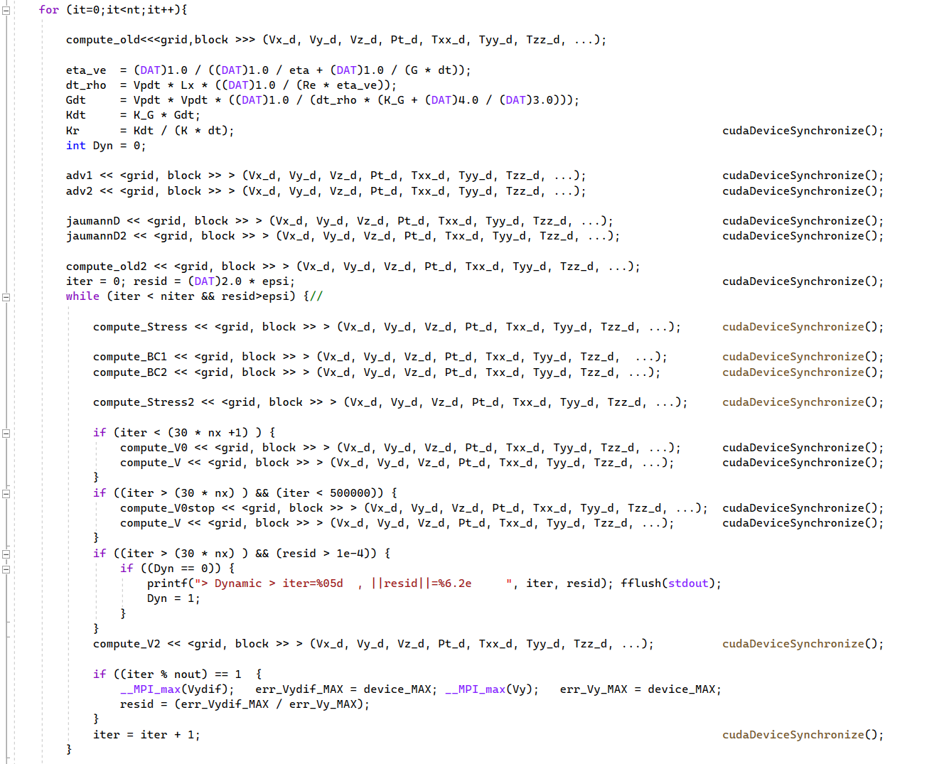
We use the CUDA C language to implement the numerical solver. The solver consists of two time loops: the first time loop belongs to physical time $t$ whereas the second time loop belongs to the pseudo-time $\widetilde{t}$ integration to achieve a steady-state solution at each discrete physical time step. Figure 1 shows the time loop computations of compressible visco-elasto-plastic solver for a single GPU CUDA C code implementation. The time loops call several kernels (GPU functions) to sequentially solve the system of equations (33)-(35).

We calculated our results using several computing systems. The code prototyping was developed on a laptop hosting $13^{th}$ Gen Intel Core i9-13900HX CPU (64GB RAM) and NVIDIA GeForce RTX 4090 (16GB) laptop GPU. Large scale two- and three- dimensional simulations were conducted on an NVIDIA DGX-1 - like node hosting 4 NVIDIA Ampere A100 (80GB) GPUs and AMD EPYC 7742 (512GB RAM) Server Processor.

The visco-elasto-plastic solver is represented by the system of equations (33)-(35). The computational domain is a cube (or square in 2D) with dimensions $x,y,z\in[0,L_{x}]\times[0,L_{y}]\times[0,L_{z}]$ (in 2D $x,y\in[0,L_{x}]\times[0,L_{y}]$). All simulations presented in this study have been performed using a simple initial model configuration. The pure shear boundary conditions are applied by prescribing velocities at all boundaries. In two-dimensions, we set

$$v_{x}=ax$$

(46)

and

$$v_{y}=-ay,$$

(47)

In three-dimensions, we prescribe

$$v_{x}=ax,$$

(48)

$$v_{y}=-ay,$$

(49)

and

$$v_{z}=0,$$

(50)

which corresponds to the extension in x-dimension and compression in y- dimension. In the brittle regime (elastic domain), we impose loading increments applied to the strain components. In the ductile regime (viscous domain), we impose velocity increments. At all boundaries, free-slip boundary conditions are implemented.

We introduce the non-dimensional shear modulus and non-dimensional cohesion:

	$\displaystyle\bar{G}$	$\displaystyle=G/G_{0},$		(51)
	$\displaystyle\bar{c}$	$\displaystyle=c/c_{0}.$		(52)

In all simulations, except for the first series of computations (section ”Symmetry versus non-symmetry”), the following initial conditions and heterogeneities are employed. All initial conditions (pressure, deviatoric stress and strain) are set equal to zero. We set anomalies to the non-dimensional shear modulus $\bar{G}$ and cohesion $\bar{c}$. The shear modulus $\bar{G}$ is represented by a Gaussian distribution with the lowest value ($\bar{G}=1$) attributed to the center of the model, $\bar{G}$ gradually increases towards the walls of the model reaching the highest value of $\bar{G}=1.2$. The non-dimensional cohesion $\bar{c}$ has a similar Gaussian distribution with the lowest value ($\bar{c}=0.2\cdot 10^{-2}$) in the center of the model; in addition, a sharp jump to the higher value ($\bar{c}=0.4\cdot 10^{-2}$) is introduced near the walls of the model to eliminate possible boundary effects. The angle of internal friction is $\phi=30^{\circ}$ in all computations.

We use $L^{\infty}$ metric space for measuring the error:

$$L^{\infty}(\bm{V})=\max_{i}{|V_{i}|}$$

(53)

The relative error is calculated as

$$\epsilon_{\mathrm{rel}}=\frac{\max_{i}\{|V_{i}-V_{i}^{it}|\}}{\max_{i}\{|V_{i}|\}}$$

(54)

and the residual equation error is

$$\epsilon_{\mathrm{abs}}=\max_{i}\{|-\nabla p_{i}+\nabla\cdot\bm{\tau}_{i}|\}.$$

(55)

Figure 2 shows a typical evolution of the relative $L^{\infty}$ norm of residuals throughout the localization phase. The relative residual error $\epsilon_{\mathrm{rel}}$ for a (typical) $10^{th}$ strain increment of a simulation involving $1535\times 767$ cells is shown in Figure 2a. The absolute residual error $\epsilon_{\mathrm{abs}}$ for the same simulation is shown in Figure 2b.

The first series of computations are carried using compressible visco-elasto-plastic equations. The Deborah number is set to $De=10^{6}$ which corresponds to the brittle domain (elastic limit). We set a circular pressure anomaly to the center of the model ($p=\bar{c}/2$ inside the perturbation, $p=0$ outside the perturbation). We set the shear modulus $\bar{G}=1$ and the cohesion $\bar{c}=0.2\cdot 10^{-2}$ in the entire model domain. Figure 4ae shows the integrated stress over one vertical line segment versus time. Figure 4bc shows the second invariant of the accumulated strain $\varepsilon_{II}$ for two different temporal resolutions.

First, we run two low-resolution simulations of $383\times 191$ grid cells. Note that in this example, for simplicity, we exclude the Jaumann derivative. In the first run, only 7 increments in time were performed (with a large time step) (Figure 4b). At each time increment we fully converged to the desired relative error $\epsilon_{\mathrm{rel}}$ of $10^{-12}$ (equation (54)). Four shear bands evolve starting from the pressure anomaly and grow towards the walls of the model. An incorrect symmetric strain localization pattern is clearly visible. Contrary, Figure 4c corresponds to the calculation of 180 increments in time (with a small time step), at each increment the iterations converged to the desired relative error $\epsilon_{\mathrm{rel}}$ of $10^{-12}$. Two shear bands develop starting from the pressure anomaly and grow towards the walls of the model, than reflect. The resulting solution exhibits a correct non-symmetric strain localization pattern. Note, that the non-symmetric solution corresponds to the sharper stress drop (and lower stress) than the symmetric solution (Figure 4a). To further investigate the difference, we plot the displacement increments corresponding to the stress drop $\Delta u_{x}=u_{x}(2)-u_{x}(1)$ for both, symmetric and non-symmetric solutions (Figure 4fg). Sharp discontinuances observed in both solutions. Note that we observe stress drops in deforming medium even without material strain softening or dynamic reduction of the static friction coefficient.

In this set of experiments, we investigate both the temporal and spatial resolutions, as well as, the Jaumann derivative. Figure 5 shows the integrated stress over one vertical line segment versus the number of increments and the second invariant of the accumulated strain $\varepsilon_{II}$ for different temporal and spatial resolutions. Two to four shear bands develop starting from the pressure anomaly (Figure 5bdfh). First, we run a low-resolution simulation of $191\times 95$ grid cells, 8 increments in total (Figure 5b). At each time increment we fully converged to the desired relative error $\epsilon_{\mathrm{rel}}$ of $10^{-12}$. A symmetric strain localization pattern is clearly visible. Then, we run a simulation for the resolution of $383\times 191$ grid cells, 8 increments in total (Figure 5d). At each time increment we fully converged to the desired relative error $\epsilon_{\mathrm{rel}}$ of $10^{-12}$. Again, a symmetric strain localization pattern can be observed. For the next simulation, we increased the temporal resolution by increasing the number of loading steps (i.e., by decreasing the time step) and performed 180 increments. At each increment the simulation converged to the desired relative error $\epsilon_{\mathrm{rel}}$ of $10^{-12}$. As a result, a correct non-symmetric strain localization pattern is visible (Figure 5f). Note, that the stress drop is also visible in Figure 5e compared to previous simulations in Figures 5ac. In a similar way, we performed a simulation of $1535\times 767$ grid cells and kept the same temporal resolution. Again, a correct non-symmetric strain localization pattern (Figure 5h) as well as the stress drop (Figure 5g) are visible.

In the second set of simulations, we explore the incompressible elastic and viscous limits of the incompressible visco-elasto-plastic equations. Figure 7a shows the initial setup for cohesion, $\bar{c}$; shear modulus, $\bar{G}$, has a constant value of $1$. By setting the Deborah number to the high values $De=10^{6}$, we reach the elastic limit (brittle domain). Figure 8a-c shows the accumulated strain $\varepsilon_{II}$, the velocity field in $x$-direction $v_{x}$ and pressure $p$ for the model configuration corresponding to the elastic limit after 30 loading increments with $\Delta t=0.4\cdot 10^{-5}$. The model resolution is $N=511^{2}$ grid cells. The strain localization develops at the center of the model with one initial shear band. The shear band is growing towards the walls of the model as the strain increments evolve in physical time. The velocity field $v_{x}$ clearly shows a discontinuity along the shear band (Figure 8b).

Alternatively, by setting the Deborah number to the low value $De=10^{-4}$, the viscous limit is reached (ductile domain). Figure 8d-f shows the accumulated strain $\varepsilon_{II}$, the velocity field in $x$-direction $v_{x}$ and pressure $p$ after 10 loading increments applied to velocity with $a=1.01$. As in the elastic limit, the velocity field $v_{x}$ exhibits a discontinuity along the shear band (Figure 8e). The behavior of the strain localization evolution is similar in both, elastic and viscous, regimes. The only difference between regimes is that in the elastic domain the strain increments are prescribed (equivalent to increments in displacement) whereas in the viscous domain velocity increments are prescribed.

Figure 9 shows the simulation results of compressible visco-elasto-plastic equations in the brittle domain after 10 loading increments with $\Delta t=0.2\cdot 10^{-5}$. The model resolution is $N=10239^{2}\approx 105.000.000$ grid cells. Figure 7 shows the initial setup for cohesion, $\bar{c}$, and shear modulus, $\bar{G}$. The accumulated strain $\varepsilon_{II}$, the displacement in $x$-direction $u_{x}$ and pressure $p$ are shown. Similarly to the previous simulations of incompressible equations, a single shear band can be observed. However, the orientation is different; according to our numerical experiments, the orientation might be different for any model configuration. It is clearly visible, that the shear band grows under two different angles with a sharp discontinuity between them.

References

- Aagaard et al. (2013) Aagaard, B. T., Knepley, M. G., and Williams, C. A. (2013). A domain decomposition approach to implementing fault slip in finite-element models of quasi-static and dynamic crustal deformation. Journal of Geophysical Research: Solid Earth, 118(6):3059–3079.
- Alkhimenkov et al. (2021a) Alkhimenkov, Y., Khakimova, L., and Podladchikov, Y. (2021a). Stability of discrete schemes of biot’s poroelastic equations. Geophysical Journal International, 225(1):354–377.
- Alkhimenkov et al. (2021b) Alkhimenkov, Y., Räss, L., Khakimova, L., Quintal, B., and Podladchikov, Y. (2021b). Resolving wave propagation in anisotropic poroelastic media using graphical processing units (gpus). Journal of Geophysical Research: Solid Earth, 126(7):e2020JB021175.
- Allison and Dunham (2018) Allison, K. L. and Dunham, E. M. (2018). Earthquake cycle simulations with rate-and-state friction and power-law viscoelasticity. Tectonophysics, 733:232–256.
- Balay et al. (2019) Balay, S., Abhyankar, S., Adams, M., Brown, J., Brune, P., Buschelman, K., Dalcin, L., Dener, A., Eijkhout, V., Gropp, W., et al. (2019). Petsc users manual.
- Baumgardner (1985) Baumgardner, J. R. (1985). Three-dimensional treatment of convective flow in the earth’s mantle. Journal of Statistical Physics, 39:501–511.
- Braun et al. (2008) Braun, J., Thieulot, C., Fullsack, P., DeKool, M., Beaumont, C., and Huismans, R. (2008). Douar: A new three-dimensional creeping flow numerical model for the solution of geological problems. Physics of the Earth and Planetary Interiors, 171(1-4):76–91.
- Buck (1993) Buck, W. R. (1993). Effect of lithospheric thickness on the formation of high-and low-angle normal faults. Geology, 21(10):933–936.
- Burstedde et al. (2008) Burstedde, C., Ghattas, O., Gurnis, M., Stadler, G., Tan, E., Tu, T., Wilcox, L. C., and Zhong, S. (2008). Scalable adaptive mantle convection simulation on petascale supercomputers. In SC’08: Proceedings of the 2008 ACM/IEEE Conference on Supercomputing, pages 1–15. IEEE.
- Cundall (1989) Cundall, P. (1989). Numerical experiments on localization in frictional materials. Ingenieur-archiv, 59:148–159.
- Cundall (1990) Cundall, P. (1990). Numerical modelling of jointed and faulted rock. In International conference on mechanics of jointed and faulted rock, pages 11–18.
- Dabrowski et al. (2008) Dabrowski, M., Krotkiewski, M., and Schmid, D. (2008). Milamin: Matlab-based finite element method solver for large problems. Geochemistry, Geophysics, Geosystems, 9(4).
- Dal Zilio et al. (2022) Dal Zilio, L., Lapusta, N., Avouac, J.-P., and Gerya, T. (2022). Subduction earthquake sequences in a non-linear visco-elasto-plastic megathrust. Geophysical Journal International, 229(2):1098–1121.
- Davies et al. (2013) Davies, D. R., Davies, J. H., Bollada, P. C., Hassan, O., Morgan, K., and Nithiarasu, P. (2013). A hierarchical mesh refinement technique for global 3-d spherical mantle convection modelling. Geoscientific Model Development, 6(4):1095–1107.
- Davies et al. (2011) Davies, D. R., Wilson, C. R., and Kramer, S. C. (2011). Fluidity: A fully unstructured anisotropic adaptive mesh computational modeling framework for geodynamics. Geochemistry, Geophysics, Geosystems, 12(6).
- De Borst et al. (2012) De Borst, R., Crisfield, M. A., Remmers, J. J., and Verhoosel, C. V. (2012). Nonlinear finite element analysis of solids and structures. John Wiley & Sons.
- de Borst and Duretz (2020) de Borst, R. and Duretz, T. (2020). On viscoplastic regularisation of strain-softening rocks and soils. International Journal for Numerical and Analytical Methods in Geomechanics, 44(6):890–903.
- de Souza Neto et al. (2011) de Souza Neto, E. A., Peric, D., and Owen, D. R. (2011). Computational methods for plasticity: theory and applications. John Wiley & Sons.
- Deng et al. (1998) Deng, J., Gurnis, M., Kanamori, H., and Hauksson, E. (1998). Viscoelastic flow in the lower crust after the 1992 landers, california, earthquake. Science, 282(5394):1689–1692.
- Dieterich (1978) Dieterich, J. H. (1978). Time-dependent friction and the mechanics of stick-slip. Rock friction and earthquake prediction, pages 790–806.
- Dieterich (1979) Dieterich, J. H. (1979). Modeling of rock friction: 1. experimental results and constitutive equations. Journal of Geophysical Research: Solid Earth, 84(B5):2161–2168.
- Dormy and Tarantola (1995) Dormy, E. and Tarantola, A. (1995). Numerical simulation of elastic wave propagation using a finite volume method. Journal of Geophysical Research: Solid Earth, 100(B2):2123–2133.
- Drucker and Prager (1952) Drucker, D. C. and Prager, W. (1952). Soil mechanics and plastic analysis or limit design. Quarterly of applied mathematics, 10(2):157–165.
- Duretz et al. (2019a) Duretz, T., de Borst, R., and Le Pourhiet, L. (2019a). Finite thickness of shear bands in frictional viscoplasticity and implications for lithosphere dynamics. Geochemistry, Geophysics, Geosystems, 20(11):5598–5616.
- Duretz et al. (2021) Duretz, T., de Borst, R., and Yamato, P. (2021). Modeling lithospheric deformation using a compressible visco-elasto-viscoplastic rheology and the effective viscosity approach. Geochemistry, Geophysics, Geosystems, 22(8):e2021GC009675.
- Duretz et al. (2020) Duretz, T., de Borst, R., Yamato, P., and Le Pourhiet, L. (2020). Toward robust and predictive geodynamic modeling: The way forward in frictional plasticity. Geophysical Research Letters, 47(5):e2019GL086027.
- Duretz et al. (2019b) Duretz, T., Räss, L., Podladchikov, Y., and Schmalholz, S. (2019b). Resolving thermomechanical coupling in two and three dimensions: spontaneous strain localization owing to shear heating. Geophysical Journal International, 216(1):365–379.
- Farrington et al. (2014) Farrington, R., Moresi, L.-N., and Capitanio, F. A. (2014). The role of viscoelasticity in subducting plates. Geochemistry, Geophysics, Geosystems, 15(11):4291–4304.
- Forsyth (1992) Forsyth, D. W. (1992). Finite extension and low-angle normal faulting. Geology, 20(1):27–30.
- Frankel (1950) Frankel, S. P. (1950). Convergence rates of iterative treatments of partial differential equations. Mathematics of Computation, 4(30):65–75.
- Gabriel et al. (2013) Gabriel, A.-A., Ampuero, J.-P., Dalguer, L., and Mai, P. M. (2013). Source properties of dynamic rupture pulses with off-fault plasticity. Journal of Geophysical Research: Solid Earth, 118(8):4117–4126.
- Gerya and Yuen (2007) Gerya, T. V. and Yuen, D. A. (2007). Robust characteristics method for modelling multiphase visco-elasto-plastic thermo-mechanical problems. Physics of the Earth and Planetary Interiors, 163(1-4):83–105.
- Glerum et al. (2018) Glerum, A., Thieulot, C., Fraters, M., Blom, C., and Spakman, W. (2018). Nonlinear viscoplasticity in aspect: benchmarking and applications to subduction. Solid Earth, 9(2):267–294.
- Happel and Brenner (1983) Happel, J. and Brenner, H. (1983). Low Reynolds number hydrodynamics: with special applications to particulate media, volume 1. Springer Science & Business Media.
- Hill (1950) Hill, R. (1950). The mathematical theory of plasticity. Clarendon Press, Oxford.
- Hill (1958) Hill, R. (1958). A general theory of uniqueness and stability in elastic-plastic solids. Journal of the Mechanics and Physics of Solids, 6(3):236–249.
- Jaquet et al. (2016) Jaquet, Y., Duretz, T., and Schmalholz, S. M. (2016). Dramatic effect of elasticity on thermal softening and strain localization during lithospheric shortening. Geophysical Journal International, 204(2):780–784.
- Kachanov (1974) Kachanov, L. M. (1974). Fundamentals of the Theory of Plasticity. MIR Publishers, Moscow.
- Kaneko and Fialko (2011) Kaneko, Y. and Fialko, Y. (2011). Shallow slip deficit due to large strike-slip earthquakes in dynamic rupture simulations with elasto-plastic off-fault response. Geophysical Journal International, 186(3):1389–1403.
- Kaus (2010) Kaus, B. J. (2010). Factors that control the angle of shear bands in geodynamic numerical models of brittle deformation. Tectonophysics, 484(1-4):36–47.
- Kaus and Podladchikov (2006) Kaus, B. J. and Podladchikov, Y. Y. (2006). Initiation of localized shear zones in viscoelastoplastic rocks. Journal of Geophysical Research: Solid Earth, 111(B4).
- Kronbichler et al. (2012) Kronbichler, M., Heister, T., and Bangerth, W. (2012). High accuracy mantle convection simulation through modern numerical methods. Geophysical Journal International, 191(1):12–29.
- Lavier et al. (1999) Lavier, L. L., Roger Buck, W., and Poliakov, A. N. (1999). Self-consistent rolling-hinge model for the evolution of large-offset low-angle normal faults. Geology, 27(12):1127–1130.
- Lemiale et al. (2008) Lemiale, V., Mühlhaus, H.-B., Moresi, L., and Stafford, J. (2008). Shear banding analysis of plastic models formulated for incompressible viscous flows. Physics of the Earth and Planetary Interiors, 171(1-4):177–186.
- LeVeque (1992) LeVeque, R. J. (1992). Numerical methods for conservation laws, volume 132. Springer.
- May et al. (2015) May, D. A., Brown, J., and Le Pourhiet, L. (2015). A scalable, matrix-free multigrid preconditioner for finite element discretizations of heterogeneous stokes flow. Computer methods in applied mechanics and engineering, 290:496–523.
- May and Moresi (2008) May, D. A. and Moresi, L. (2008). Preconditioned iterative methods for stokes flow problems arising in computational geodynamics. Physics of the Earth and Planetary Interiors, 171(1-4):33–47.
- Minakov and Yarushina (2021) Minakov, A. and Yarushina, V. (2021). Elastoplastic source model for microseismicity and acoustic emission. Geophysical Journal International, 227(1):33–53.
- Moczo et al. (2007) Moczo, P., Robertsson, J. O., and Eisner, L. (2007). The finite-difference time-domain method for modeling of seismic wave propagation. Advances in geophysics, 48:421–516.
- Moresi et al. (2007a) Moresi, L., Mühlhaus, H.-B., Lemiale, V., and May, D. (2007a). Incompressible viscous formulations for deformation and yielding of the lithosphere. Geological Society, London, Special Publications, 282(1):457–472.
- Moresi et al. (2007b) Moresi, L., Quenette, S., Lemiale, V., Meriaux, C., Appelbe, B., and Mühlhaus, H.-B. (2007b). Computational approaches to studying non-linear dynamics of the crust and mantle. Physics of the Earth and Planetary Interiors, 163(1-4):69–82.
- Moresi et al. (1996) Moresi, L., Zhong, S., and Gurnis, M. (1996). The accuracy of finite element solutions of stokes’s flow with strongly varying viscosity. Physics of the Earth and Planetary Interiors, 97(1-4):83–94.
- Olive et al. (2016) Olive, J.-A., Behn, M. D., Mittelstaedt, E., Ito, G., and Klein, B. Z. (2016). The role of elasticity in simulating long-term tectonic extension. Geophysical Journal International, 205(2):728–743.
- Omlin et al. (2017) Omlin, S., Malvoisin, B., and Podladchikov, Y. Y. (2017). Pore fluid extraction by reactive solitary waves in 3-d. Geophysical Research Letters, 44(18):9267–9275.
- Omlin et al. (2018) Omlin, S., Räss, L., and Podladchikov, Y. Y. (2018). Simulation of three-dimensional viscoelastic deformation coupled to porous fluid flow. Tectonophysics, 746:695–701.
- Poliakov and Herrmann (1994) Poliakov, A. and Herrmann, H. (1994). Self-organized criticality of plastic shear bands in rocks. Geophysical Research Letters, 21(19):2143–2146.
- Poliakov et al. (1993) Poliakov, A., Podladchikov, Y., and Talbot, C. (1993). Initiation of salt diapirs with frictional overburdens: numerical experiments. Tectonophysics, 228(3-4):199–210.
- Poliakov et al. (1994) Poliakov, A. N., Herrmann, H. J., Podladchikov, Y. Y., and Roux, S. (1994). Fractal plastic shear bands. Fractals, 2(04):567–581.
- Popov and Sobolev (2008) Popov, A. and Sobolev, S. V. (2008). Slim3d: A tool for three-dimensional thermomechanical modeling of lithospheric deformation with elasto-visco-plastic rheology. Physics of the earth and planetary interiors, 171(1-4):55–75.
- Pranger et al. (2022) Pranger, C., Sanan, P., May, D. A., Le Pourhiet, L., and Gabriel, A.-A. (2022). Rate and state friction as a spatially regularized transient viscous flow law. Journal of Geophysical Research: Solid Earth, 127(6):e2021JB023511.
- Räss et al. (2019) Räss, L., Duretz, T., and Podladchikov, Y. (2019). Resolving hydromechanical coupling in two and three dimensions: spontaneous channelling of porous fluids owing to decompaction weakening. Geophysical Journal International, 218(3):1591–1616.
- Räss et al. (2020) Räss, L., Licul, A., Herman, F., Podladchikov, Y. Y., and Suckale, J. (2020). Modelling thermomechanical ice deformation using an implicit pseudo-transient method (fastice v1. 0) based on graphical processing units (gpus). Geoscientific Model Development, 13(3):955–976.
- Räss et al. (2022) Räss, L., Utkin, I., Duretz, T., Omlin, S., and Podladchikov, Y. Y. (2022). Assessing the robustness and scalability of the accelerated pseudo-transient method. Geoscientific Model Development, 15(14):5757–5786.
- Rice and Rudnicki (1980) Rice, J. R. and Rudnicki, J. (1980). A note on some features of the theory of localization of deformation. International Journal of solids and structures, 16(7):597–605.
- Rudnicki and Rice (1975) Rudnicki, J. W. and Rice, J. (1975). Conditions for the localization of deformation in pressure-sensitive dilatant materials. Journal of the Mechanics and Physics of Solids, 23(6):371–394.
- Ruina (1983) Ruina, A. (1983). Slip instability and state variable friction laws. Journal of Geophysical Research: Solid Earth, 88(B12):10359–10370.
- Scholz (2019) Scholz, C. H. (2019). The mechanics of earthquakes and faulting. Cambridge university press.
- Spiegelman et al. (2016) Spiegelman, M., May, D. A., and Wilson, C. R. (2016). On the solvability of incompressible stokes with viscoplastic rheologies in geodynamics. Geochemistry, Geophysics, Geosystems, 17(6):2213–2238.
- Sulem and Vardoulakis (1995) Sulem, J. and Vardoulakis, I. (1995). Bifurcation analysis in geomechanics. CRC Press.
- Tackley (1996) Tackley, P. J. (1996). Effects of strongly variable viscosity on three-dimensional compressible convection in planetary mantles. Journal of Geophysical Research: Solid Earth, 101(B2):3311–3332.
- Tackley (2008) Tackley, P. J. (2008). Modelling compressible mantle convection with large viscosity contrasts in a three-dimensional spherical shell using the yin-yang grid. Physics of the Earth and Planetary Interiors, 171(1-4):7–18.
- Templeton and Rice (2008) Templeton, E. L. and Rice, J. R. (2008). Off-fault plasticity and earthquake rupture dynamics: 1. dry materials or neglect of fluid pressure changes. Journal of Geophysical Research: Solid Earth, 113(B9).
- Thieulot (2011) Thieulot, C. (2011). Fantom: Two-and three-dimensional numerical modelling of creeping flows for the solution of geological problems. Physics of the Earth and Planetary Interiors, 188(1-2):47–68.
- Tong and Lavier (2018) Tong, X. and Lavier, L. L. (2018). Simulation of slip transients and earthquakes in finite thickness shear zones with a plastic formulation. Nature communications, 9(1):3893.
- Turcotte and Schubert (2002) Turcotte, D. L. and Schubert, G. (2002). Geodynamics. Cambridge university press.
- Uphoff et al. (2023) Uphoff, C., May, D. A., and Gabriel, A.-A. (2023). A discontinuous galerkin method for sequences of earthquakes and aseismic slip on multiple faults using unstructured curvilinear grids. Geophysical Journal International, 233(1):586–626.
- Vardoulakis et al. (1978) Vardoulakis, I., Goldscheider, M., and Gudehus, G. (1978). Formation of shear bands in sand bodies as a bifurcation problem. International Journal for numerical and analytical methods in Geomechanics, 2(2):99–128.
- Vermeer (1990) Vermeer, P. (1990). The orientation of shear bands in biaxial tests. Géotechnique, 40(2):223–236.
- Vermeer and De Borst (1984) Vermeer, P. A. and De Borst, R. (1984). Non-associated plasticity for soils, concrete and rock. HERON, 29 (3), 1984.
- Virieux (1986) Virieux, J. (1986). P-sv wave propagation in heterogeneous media: Velocity-stress finite-difference method. Geophysics, 51(4):889–901.
- Virieux and Madariaga (1982) Virieux, J. and Madariaga, R. (1982). Dynamic faulting studied by a finite difference method. Bulletin of the Seismological Society of America, 72(2):345–369.
- Wilson et al. (2017) Wilson, C. R., Spiegelman, M., and van Keken, P. E. (2017). Terra ferma: The t ransparent f inite e lement r apid m odel a ssembler for multiphysics problems in e arth sciences. Geochemistry, Geophysics, Geosystems, 18(2):769–810.
- Wollherr et al. (2018) Wollherr, S., Gabriel, A.-A., and Uphoff, C. (2018). Off-fault plasticity in three-dimensional dynamic rupture simulations using a modal discontinuous galerkin method on unstructured meshes: implementation, verification and application. Geophysical Journal International, 214(3):1556–1584.
- Zienkiewicz and Taylor (2005) Zienkiewicz, O. C. and Taylor, R. L. (2005). The finite element method for solid and structural mechanics. Elsevier.
- Zienkiewicz et al. (2013) Zienkiewicz, O. C., Taylor, R. L., and Nithiarasu, P. (2013). The finite element method for fluid dynamics. Butterworth-Heinemann.