Pseudo channel reciprocity in FDD satellite channels
Abstract
Channel reciprocity can significantly reduce the overhead of obtaining channel-state information at the transmitter (CSIT). However, true reciprocity only exists in time division duplex (TDD). In this paper, we propose a novel tracking method that exploits implicit reciprocity in FDD line-of-sight (LOS) channels as in low-earth-orbit (LEO) satellite communication (SatCom). This channel reciprocity, dubbed pseudo-reciprocity, is crucial for applying multiple-user multiple-input multiple-output (MU-MIMO) to SatCom, which requires CSIT. We consider an LEO SatCom system where multiple satellites communicate with a multi-antenna land terminal (LT). In this innovative method, the LT can track the downlink channel changes and use them to estimate the uplink channels. The proposed method achieves precoding performance that is comparable to precoding with full CSIT knowledge. Furthermore, the use of pseudo reciprocity typically requires only initial CSIT feedback when the satellite rises. Over very long periods of time, pseudo reciprocity can fail as a result of phase ambiguity, which is referred to as cycle slip. We thus also present a closed-form approximation for the expected time until cycle slip, which indicates that in normal operating conditions, these cycle slips are extremely rare. Our numerical results provide strong support for the derived theory.
Index Terms:
MIMO, SatCom, LEO satellites, Reciprocity.I Introduction
Satellite communication (SatCom) systems are essential for universal coverage since they do not require terrestrial infrastructure. For this reason, commercial and public institutions plan to deploy thousands of low-earth-orbit (LEO) satellites over the next decade. These systems must have high throughput to justify such a massive investment. MIMO technology and in particular multi-user MIMO (MIMO) are vital for overcoming this challenge in SatCom [1, 2, 3].
MU-MIMO can dramatically enhance throughput, but requires both channel-state information at the receiver (CSIR) and channel-state information at the transmitter (CSIT) [4, 5]. The receiver usually estimates the CSIR through received pilot sequences. Obtaining CSIT, on the other hand, is more challenging.
In time division duplex (TDD) systems, CSIT can be obtained using channel reciprocity (e.g., [6, 7]). In these systems, the uplink and downlink channels are in the same frequency band and hence experience the same channel (reciprocal). Thus, the channel estimated during the receive time slot (as CSIR) can be used in the transmit time slot (as CSIT). Note that the receive hardware and transmit hardware are not reciprocal. Thus, the use of channel reciprocity requires hardware calibration [8, 9].
In frequency division duplex (FDD) systems, the uplink and downlink channels use different frequencies and hence channel reciprocity does not hold. Note that the uplink and downlink channels typically have some common properties, such as angular power spectrum, spatial covariance matrix, delay, and multipath angles [10, 11]. These reciprocal properties can be used for user selection [12] or to reduce the feedback rate [13, 14, 15]. However, since the channel gains are not reciprocal, all these schemes still require significant feedback.
Although channel reciprocity in FDD systems may initially appear unattainable, it is, in fact, possible within SatCom systems. The SatCom channel is predominantly characterized by a LOS component, which changes over time. This LOS channel allows for the inference of one link direction based on the other, thereby enabling channel estimation through reciprocity. Consequently, SatCom systems offer a unique opportunity for exploiting channel reciprocity in the FDD setup.
In a LOS channel, the channel phase is determined by the delay and the carrier frequency11 1 The effects of transmitter hardware, antenna gains, and atmospheric and rain attenuation obviously affect the phase. But, we are interested in the phase changes between the antennas in the same equipment, which experience the same effects.. Thus, exact knowledge of the delay is sufficient to achieve CSI. But in most practical scenarios, it is not feasible to estimate the delay with sufficient accuracy. Instead, the channel phase can be accurately estimated from the CSIR up to a modulo . In TDD systems, where the carrier frequency is similar in both link directions, the channel phases are also identical. Hence, a good estimation of the modulo phase is sufficient to be able to tap channel reciprocity.
However, achieving channel reciprocity in FDD systems is more complicated and not as straightforward as in TDD systems. This is primarily because the uplink and downlink channels have different frequencies, resulting in unequal channel phases. Thus, knowledge of the phase modulo in one link direction is not enough for phase estimation in the other direction. So far, there is no known technique for exploiting channel reciprocity in FDD LEO SatCom.
This paper proposes an innovative scheme for exploiting channel reciprocity in LEO SatCom systems which typically have dominant line-of-sight (LOS) and employ FDD. In the proposed scheme, the land terminal (LT) estimates its uplink CSIT from its downlink CSIR, and requires only channel-state information (CSI) feedback for initialization. Our main result is based on the fact that the Doppler shift in the uplink and downlink is identical up to a multiplicative constant. Thus, using appropriate techniques, the phase variations of the uplink channel can be predicted from the estimated phase variations in the downlink channel.
We consider a network containing several LEO satellites communicating with a single multi-antenna LT. The LT estimates the downlink channels (CSIR) via pilot sequences sent by the satellites. From this CSIR, the LT calculates its received beamformer for extracting each satellite’s data stream. Moreover, the LT uses its CSIR to track the uplink channel (CSIT) by tracking the downlink channel phase variations. Finally, the LT uses this CSIT to calculate a zero-forcing (ZF) precoding matrix for sending data simultaneously to the satellites in the uplink.
Notations: We denote Matrices and vectors by boldface upper and lower case letters, respectively. We use , and for the conjugate and transpose operations, respectively, and and , for the expectation and variance operations, respectively. Let , then we defined its modulo as
| (1) |
For , we denote its phase modulo by .
II System Model
We consider a FDD satellite communication network where a fixed land terminal (LT) with antennas communicates simultaneously with LEO satellites, each having a single antenna. In the downlink, all satellites send pilots periodically whereas in the uplink, whenever the LT transmits, it sends independent data streams simultaneously to the satellites.

The LT tracks the downlink channel phase variations from the pilot sent by each satellite. Based on this CSIR, the LT extracts each satellite data stream using received beamforming. In the uplink, on the other hand, the LT uses transmit-beamforming to null interference from signals designated to other satellites. To do so, the LT needs to extract the uplink CSIT from the downlink CSIR.
II-A Downlink
The LT uses the pilot symbols transmitted by the satellites to construct a matrix channel estimation. The channel estimation for the -th symbol can be written as:
| (2) |
where is the LT downlink carrier frequency, is the satellite downlink hardware frequency-offset, is the distance between satellite- and the -th LT antenna at sample , is the phase offset related to satellite , is the symbol duration, is the speed of light and is a constant expressing the effect of transmitter hardware, antenna gains, and atmospheric and rain attenuation for satellite 22 2 The channel factoring in (2) includes the standard approximation, where we assume that is negligible compared to but is not negligible.. The estimation error term, is composed of identical independent distributed (i.i.d.) complex Gaussian random variables with zero mean and variance of .
The matrix also can be written as
| (3) |
where
| (4) |
contains only phase information, where
| (5) |
and
| (6) |
is a diagonal matrix containing the amplitude for all channel entries corresponding to the same satellite.
Note that matrix changes very slowly, and much slower than matrix . Therefore, the LT has a long time to estimate the matrix , and we assume that this estimation results in a negligible estimation error.
II-B Uplink
The LT transmits independent data streams, each designated for a distinct satellite. The baseband output signal at antenna is
| (7) |
where is the -th symbol transmitted by antenna and is the normalized pulse shape, which is free of inter symbol interference (ISI). Thus, the pulse auto-correlation satisfies . The corresponding passband signal is
| (8) |
where is the uplink carrier frequency. The received passband signal at satellite is
| (9) |
where is a complex circular white Gaussian noise with two sided spectral density , and is a constant expressing the effect of transmitter hardware, antenna gains, and atmospheric and rain attenuation. The received baseband signal at satellite after multiplying by and applying LPF is
Using the standard approximation again, we can replace by in the argument of (but not in the exponent). In addition, the sampling instances at the output of the match filter on satellite are where . The resulting samples are
As the pulse shape is normalized and ISI free, the noise is a complex circular white Gaussian with variance .
We assume that the gap between the distances from the satellite to the LT first antenna and to its -th antenna, , is neglected in the attenuation term . This small gap only affects the argument of the exponent, where it is multiplied by , hence
| (10) |
Next, we denote , and and . Thus, can be written as
| (11) |
where
Note that we write (11) with a transpose on the channel matrix for convenience (which is common in reciprocity models).
Matrix can be written as
| (12) |
where
is a diagonal matrix containing the terms that are equal for all channel elements corresponding to the same satellite, and
| (13) |
is a phase matrix, which takes into account the phase differences between LT antennas where
| (14) |
II-C Uplink ZF precoding
In the uplink, the LT employs a ZF precoding to cancel interferences between streams designated for different satellites. Let be the data symbol transmitted to satellite and be the vector of all transmitted symbols at time . This vector is precoded using the precoding matrix, , to generate: . The ZF precoding matrix is then
| (15) |
Note that the ZF precoding does not require full CSIT, , but only the phase matrix . Using the ZF precoding, the received sampled signals at the satellites are
| (16) |
To summarize, the LT can cancel interference in downlink and uplink channels as long as it has a good enough estimate of and .
III Pseudo channel reciprocity
The utilization of ZF, both in the downlink and the uplink, requires CSI. In the downlink, we assume that the LT achieves CSIR via pilot sequences. For the uplink ZF precoding, however, the LT needs CSIT, which is far more challenging than CSIR. Without channel reciprocity, CSIT requires channel estimation at the receiver and feedback, which incurs an overhead. Channel reciprocity is often used in TDD systems, where both uplink and downlink use the same carrier frequency. In our case, which includes FDD, LOS and high Doppler shifts, achieving channel reciprocity is difficult. We now propose a new scheme that utilizes downlink channel estimation to track the uplink channel. While the scheme still includes uplink channel estimation at the satellites and feedback, it can be at a significantly lower rate.
III-A problem formulation
As the matrices and are diagonal, both the ZF precoder and the ZF equalizer only require the knowledge of the matrices and , respectively. Moreover, since all the elements in the matrices and have an amplitude of , it is sufficient to study their phases. Thus, in the following, we focus on the channel phases; i.e., the phases of the elements of the matrices and . Let and be the entries of and , respectively: recall that and are the corresponding phases.
The channel estimation goal is to track using sequential estimates of . The challenge of this reciprocity procedure is that the LT does not observe estimates of the actual channel phase, but only its modulo . Thus, the goal is actual work is to track given sequential estimates of .
III-B Pseudo Reciprocity
We now propose a tracking algorithm wherein the LT extracts the uplink channel phases from the estimation of the downlink channel phases. For simplicity of presentation, in this section we present a scheme that only works when the frequency offsets between the satellites and the LT are negligible (i.e., we assume ). In the next section, we present an algorithm that also works in the presence of such frequency offset.
We first present the scheme in the absence of estimation errors, but later present a performance analysis in the presence of noise. For , the measured channel phase is
| (17) |
The LT has no information on . Thus all our schemes will require the initial feedback of a single estimate of the uplink . Once we have this feedback, we will show that it is sufficient to track to estimate .
If the LT could obtain a reasonable estimate of , it would extract to get a good estimate of . However, the LT does not estimate but rather its modulo. To address this problem, we write and as sums over phase increments
| (18) | |||||
| (19) |
We define the downlink measured phase change as
| (20) | |||||
We note that if
| (21) |
then
| (22) |
and hence equation (19) can be written as
| (23) |
Thus, Equation (23) establishes the pseudo channel reciprocity by showing that (given (21)) the uplink can be estimated from the downlink.
To show that condition (21) is reasonable in practical cases, consider a satellite with orbit radius and orbit period . By bounding the phase increments using the maximal Doppler shift at each instant, , one obtains
| (24) |
where is the velocity at time of satellite relative to antenna at the mobile. The inequality states that the relative velocity is bounded by the satellite’s orbital velocity, . For illustration, consider a LEO satellite traveling km above the LT while transmitting at a bandwidth of MHz with a GHz carrier frequency. In this case we have and
| (25) |
The top part of Fig. 2 depicts from satellite rise to satellite set, from the LT perspective. The figure shows that (25) is satisfied for every , and is tightest near the rise and set of the satellite.

In the remainder of this paper we assume that (21) holds.
III-C Estimation Error
We now also consider the presence of estimation errors, and examine the performance of the proposed scheme.
Definition 1.
Given the initial estimate and the sequence of estimates for , we define the recursive estimation procedure as
| (26) |
where .
As explained above, the amplitude of the channel changes very slowly; hence we assume that the LT has exact knowledge of . Thus, we only consider the error in the estimation of . Let,
| (27) |
where is the estimation error. Thus, the phase increment is given by
| (28) |
where is the downlink-phase estimation error. Here, we extend (21) to assume that
| (29) |
Thus, (23) becomes
| (30) |
where is the uplink-phase estimation error at . Thus, the error in is a linear combination of and ; i.e., for every , the cumulative error is composed of only three elements. This is a desired estimation, as we can track the uplink for very long time, without accumulation of noise.
Thus, the main problem in the implementation of this scheme is the probability that (29) will not hold. In this case, has an additional error of , for some . This estimation error is typically large, and cannot be recovered later, except by additional feedback. Thus, it is important to study and characterize these “jump” events. In the following subsection we present an improved tracking approach using discrete-phase-lock-loop (DPLL), and study the probability of ”jump” events (which are termed cycle slip in the context of DPLL).
III-D DPLL Pseudo Reciprocity and Cycle-Slip
The well-known DPLL is very similar in structure to the scheme in definition 1, except for the multiplication of the channel phase increments by a different constant. These different multiplicative constants aim to achieve different goals. In traditional DPLL this multiplication enables further noise reduction by taking advantage of the correlation between successive increments. In our approach, the multiplication by a constant achieves the pseudo reciprocity by converting the downlink phase increments into uplink phase increments.
Many algorithms and works show good performance using DPLL for phase tracking (see for example [16, 17, 18, 19]). Thus, we present an extended DPLL scheme that aims to achieve both the noise reduction and the pseudo reciprocity.
We use a first-order DPLL that consists of two voltage-controlled-oscillators (VCO), one for the downlink phase estimation and one for the uplink, as depicted in Fig. 3. The output of the downlink VCO is used to close the DPLL loop. It also produces the improved channel phase estimate, . The second VCO is used to generate the uplink estimates, using the pseudo reciprocity increments.
The VCO has a delay of one sample time; i.e., is the estimation of the input at instant based on samples up to . The DPLL input is given in (27), and the sinusoidal phase extractor approximates the input phase by its imaginary part, given by
| (31) | |||||
where and represents the imaginary part.33 3 The phase can also be taken as the angle of the complex number. However, this phase extraction changes the error distribution, which makes the cycle slip analysis much more complicated. Note that numerical simulations show that in the low SNR regime, a complex phase extractor does not improve the DPLL tracking performance compared to the sinusoidal phase extractor.
The downlink channel phase estimates are the output of the first VCO
| (32) | |||||
whereas the uplink channel phase estimates are the output of the second VCO
| (33) |
Using our single channel feedback (for each antenna) we set . Thus, we can denote the downlink channel phase estimation error of the DPLL at sample as
| (34) |
Note that both and are not wrapped by modulo (i.e., they can take values outside the range ).
Definition 2.
Given the error at each sample , we define a cycle-slip as the event where
| (35) |
Note that (35) is the complementary condition to (29). Thus, the pseudo reciprocity holds as long as there is no cycle slip. To illustrate the pseudo reciprocity sensitivity to a cycle-slip, we consider an antenna of a single satellite and a single antenna at the LT. The LT uses DPLL to estimate the downlink and uplink channel phases based on the downlink channel pilot sequences. Fig. 4 shows the estimation errors for the downlink and for the uplink. In each direction, we plot two errors, the actual error ( in blue) and the modulo error (in red). As shown by the actual downlink error (in blue), a cycle-slip occurs in the downlink channel phase, around time . As a result, the actual error of the uplink also suffers from a cycle-slip event. The difference between the downlink and uplink channel phases performance is seen in the modulo error. The cycle-slip event does not affect the estimation of the downlink channel phases, but does affect the estimation of the uplink channel phases by a significant factor of .

To sum up, if the LT successively keeps track of the phase variations between consecutive times, then losing a -cycle only occurs in the case of a cycle slip. As long as there is no cycle sleep, the uplink channel estimation is proportional to the downlink channel error (which is typically very small). In what follows, we derive the mean number of samples to lose lock (MSL) in DPLL, which we harness to show that the reciprocity can hold for very long times.
III-E Cycle-Slip Analysis
We now derive an approximation to the MSL for the proposed system (cf. Fig 3). We start by rewriting , by substituting (31) and (32) into (34):
| (36) | |||||
where we also add and subtract . This analysis is done under the assumption of sufficiently high sampling frequency. Thus, it is reasonable to neglect
| (37) |
Using (34) for we can write
| (38) |
where
Viterbi [20] calculated the mean time for cycle slip in PLL where the input is a continuous real signal. To use the Viterbi results, note that the stochastic difference equation (38) can be seen as the Euler approximation [21] of the stochastic differential equation
| (39) |
Furthermore, the diffusion function, , and the drift function, , are infinitely continuously differentiable. Hence the process in (38) converges weakly to in (39).
Viterbi, calculated the mean time to lose lock for equation (39), which is given by
| (40) |
where
| (41) |
is the effective SNR and is the Bessel function of the first kind. By comparing (38) to (39), Equation (40) can we converted to its discrete equivalent. Thus, the MSL can be approximated by
| (42) |
Naturally, the MSL decreases monotonically with and . However, the choice of and must also take into account the tracking ability and the robustness to noise. The effect of these two quantities can be quantified for example through the mean squared error (MSE) of the steady state. As we will show, the MSL is typically very large, thus in the numerical section we chose to minimize the steady state MSE. See appendix B for details.
The MSL is also affected by the effective SNR, . Note that is a monotonically increasing function in . Furthermore, for large , we can approximate ; thus, a slight improvement in the SNR can cause a significant improvement in the MSL.
IV Reciprocity with Frequency offset
The previous section assumed no frequency offset between the satellites and the LT (). We next present an improved reciprocity procedure that works with . To do so, we rewrite the channel matrices, which involves normalizing the channel gains by the phase of antenna . That is, we rewrite the downlink channel matrix as , where
| (43) |
and
| (44) |
In the same manner, we rewrite the uplink channel matrix as , where
and
| (45) |
Matrices and are diagonal. Thus, both the ZF precoder and the ZF equalizer only require knowledge of the matrices and , respectively.
Note that all the elements in the matrices and have an amplitude of . Thus, it is sufficient to study their phases. Moreover, inspection of (44) and (45) reveals that they do not depend on the frequency error. Thus, this reciprocity scheme works as well for . In addition, (44) and (45) are only affected form the differential Doppler between the two antennas (as seen from the subtraction ). Since the antennas are relatively close, the differential Doppler is significantly smaller than the actual Doppler shift. Hence, the phase tracking in this scheme is much simpler.
Nevertheless, this scheme has two disadvantages, both related to using measurements that are phase differences between two antennas. The first disadvantage is that the noise is stronger than the phase estimation over a single antenna. However, below we show that the noise increase is negligible compared to the benefit of much slower tracking. The second disadvantage is an error distribution that is more complicated than in the previous section. This will prevent us from presenting an exact analytical study. Instead, we will present a good approximation based on a Gaussian error distribution.
To better explain this improved reciprocity scheme, we define the range differences in time and space:
| (46) |
and
| (47) |
Thus, to apply reciprocity, we need to estimate from the downlink.
The downlink channel phase in this model is
| (48) |
and the downlink measured phase change is . Thus, in the absence of noise, if
| (49) |
we can write
| (50) |
where the approximation comes from the reasonable assumption that . Hence, equation (47) can be written as
| (51) |
which shows that the reciprocity works even with and with a minimal feedback of . Note that the condition in (49) is over changes in the distance difference. As , this constraint is much more relaxed than the constraint in (21). In appendix C we show that (49) holds for any practical system. To make this advantage clearer, the top of Fig. 2 depicts for an example system setup (the top of the figure depicts for the same setup). It is obvious that is significantly smaller than . These slow variations in the phase difference (i.e., small ) can be used to improves the tracking, complexity and the MSL of the system.
The cycle slip analysis in the previous section does not apply to the scheme of this section because the estimation noise is no longer Gaussian (because we multiply each element by the conjugate of the first antenna ). Nevertheless, we found that the cycle slip analysis can produce an excellent approximation for this scheme by simply adjusting the noise variance. As in the previous section, the conditional distribution of each channel estimation is assumed to be (see Eq. (27)). Thus, for the improved scheme, the variance at the input to the DPLL is given by
| (52) | |||||
where we used (see Eq. (4)).
Substituting (52) into (42), the MSL is approximated by
| (53) |
In Fig. 8 we show that (53) is an excellent approximation for the MSL of the improved scheme.
V Numerical Results
The previous sections described our reciprocity procedure in FDD satellite communication system and derived an approximation to the MSL, which indicates the reciprocity failure probability. Here we present numerical results showing these expressions’ usefulness and accuracy.
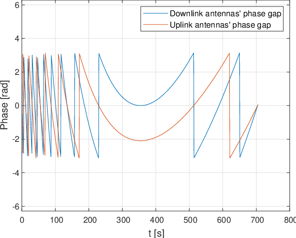
In Fig. 5, we consider a single-antenna satellite at a height of km that communicates with a double antenna LT (cm separation between the antennas). The carrier frequencies are GHz and GHz for the downlink and uplink channels, respectively. To illustrate the challenge of exploiting this uplink-downlink reciprocity, we plot the downlink and the uplink phase gaps between the LTs antennas. We aim to show no remarkable information between the downlink and uplink phase gaps. Because one may obtain that our reciprocity procedure is not innovative and can be understood quite straightforwardly. Fig. 5 shows that this interpretation is incorrect; the correlation between the downlink and uplink phase gaps is very pure and changes over time.
Fig. 6 considers an FDD satellite communication system with two single-antenna satellites communicating with a double-antenna LT. The satellites send downlink pilots periodically to the LT, whereas in the uplink, the LT sends independent data streams simultaneously to each satellite. The LT tracks the downlink channel phase variations over time and estimates the uplink channel phase to send the two data streams. We used typical SatCom parameters. The downlink and uplink carrier frequencies are GHz and GHz, respectively. In both channels we used: a s dBi transmit antenna gain, a dBi receive antenna gain, a dBm transmit power, a MHz bandwidth, and a noise power spectral density of dBm/Hz.

Fig. 6 depicts the receive SNR at one satellite for three cases. In the first one, the LT has perfect CSIT whereas the second case involves an imperfect CSIT where the LT achieves CSIT using the proposed reciprocity scheme. In both cases, the LT sends an independent data stream to each satellite simultaneously using ZF-precoding. For comparison, we consider a third case where the LT sends data to only one of the satellites using MRC precoding. Here, the LT uses its two antennas to transmit with half of the power compared to the first two cases. The figure shows that the LT estimates the uplink channel phase successfully using reciprocity with approximately the same performance as in the case of full CSIT. However, the singular values of the uplink channel phase matrix vary with time. Occasionally the matrix is well-conditioned, and the ZF-precoding works well, whereas at other times the matrix is ill conditioned so that canceling the interference to each satellite is impossible, even in the full CSIT case.
To show a match to the theory, Figs. 7 and 8 simulate the received signal at a very low SNR, even though this SNR range is not typical of satellite communication systems. The reason is that in the standard receive SNR range, the MSL is enormous and difficult to simulate. It is important to emphasize that our MSL formula (42) holds for all SNR regimes. We denote the received SNR for both cases as .

In Fig. 7, we consider one single-antenna satellite transmitting to a single antenna LT with a MHz bandwidth, a MHz sample rate (), and a carrier frequency of GHz. The LT tracks the downlink channel phase and estimates the uplink channel phase using reciprocity (cf. section III). Fig. 7 depicts the mean of the first cycle-slip in the downlink channel and the theoretical cycle-slip approximation (42) as a function of the received SNR. The figure depicts two cases: the first with a significant Doppler shift and the second with a neglected Doppler effect; each case corresponds to a specific LT-satellite instantaneous configuration. In both cases, in low SNR, the DPLL struggles to track the channel phase, so that a cycle slip occurs early. As the SNR grows, the DPLL tracking improves and the MSL increases. Because the MSL formula (42) considers a zero Doppler shift, the presence of such may cause a cumulative phase error, which explains the early cycle slip in the high Doppler case.
In Fig. 8, we consider the same setup as in Fig. 7, but with two antennas at the LT. Here, the LT tracks the downlink channel phase variations between the receive antennas and consecutive times (see (50) and (46)). The satellite transmission parameters consist of a: bandwidth of Hz , a sample rate of Hz () and carrier frequency of GHz. The downlink channel phase-variations between receive antennas contain a very small Doppler; hence, there is no cumulative Doppler phase error at the DPLL. Fig. 8 depicts the actual downlink MSL, obtained via Monte-Carlo, and the approximate (53) as a function of the received SNR. There is a good match between the simulation and the theory. The small Doppler shift enables the LT to reduce the DPLL gain hence improving the effective SNR of the DPLL. Moreover, this small Doppler enables the LT to reduce the sampling rate (only Hz!!) and still successfully track the uplink channel. According the theoretical and the numerical results, in typical SatCom SNRs, the LT usually does not experience cycle slips for the entire satellite LOS motion.
VI Conclusions
In this paper we showed the pseudo reciprocity of the uplink and downlink in FDD LOS channels. We focused on LEO SatCom systems, which are typically based on FDD and exhibit LOS dominant channels. We presented a novel scheme which allows the LT to track phase changes in the downlink channel and use them to estimate the phase changes in the uplink channel, effectively estimating the CSIT by tracking the CSIR. Our proposed pseudo-reciprocity approach achieves CSIT estimation with minimal feedback and system complexity.
Incorporating our innovative approach into SatCom systems has the potential to substantially enhance the implementation of MU-MIMO technology in SatCom. This improvement, in turn, could lead to a significant increase in data rates. The key to this enhancement lies in the fact that pseudo-reciprocity facilitates the estimation of CSIT for a large number of channels, thereby streamlining the process and improving overall performance.
We also analyzed the impact of estimation errors in the CSIR on the estimation errors in the CSIT. Our results indicate that there is no cumulative error over time, ensuring that pseudo-reciprocity remains stable for extended periods. Effectively, in most scenarios it will be sufficient to send feedback once when the satellite rises and then track the channel with small errors until the satellite sets.
To track changes in the CSIR, we proposed using a DPLL. The DPLL introduces a cycle slip probability, prompting us to calculate the Mean Time of the First Cycle Slip (MSL).
In the numerical results section, we demonstrated that using pseudo-reciprocity for precoding achieves performance comparable to precoding with full CSIT knowledge. Additionally, we confirmed that the MSL calculation aligns with our simulations. We found that within the common Signal-to-Noise Ratio (SNR) range in SatCom, cycle slips are so rare that they are not likely to occur for any satellite motion, from the satellite rise to set. Thus, our proposed pseudo-reciprocity approach offers a promising avenue for enhancing satellite communication systems while maintaining minimal complexity and feedback requirements.

Appendix A Continuous process and digital noise comparison
In this Appendix we prove that the limit of as goes to zero is a white Gaussian noise with PSD of .
Let be a general continuous function. We denote as a white Gaussian process with zero mean and PSD . In order to sample the white process, we denote the filter
| (54) |
and
| (55) |
where is the bandwidth and is the sampling gap, .
We want to show that has the same distribution as . The distribution of is a white Gaussian with zero mean and variance . Next, we calculate
| (56) |
and show that where goes to zero
| (57) |
which ends the proof.
Appendix B Calculate that minimizes the MSE
We show one way to choose that minimizes the specific downlink MSE, which is given in (34). We assume that the changes between two consecutive distinct downlink times is where is the maximum Doppler and is the sampling gap. We also use the small angle approximation . Based on these assumptions,
and the MSE is given by
| (58) | |||||
Assuming stability, and , therefore
| (59) |
and the value that gives the minimum is the solution of
| (61) |
Appendix C Doppler upper bound
In this Appendix we calculate an upper bound for the absolute value of the Doppler shift between the consecutive times and between antennas to prove that (49) is satisfied. We consider the general setup of two receive antennas on Earth and one antenna satellite as depicted in Fig. 9. We denote as the satellite velocity, as the satellite height, and are the distances between the satellite and antennas and , respectively, is the distance between the antennas, and , and as defined in Fig. 9.
The Doppler shift absolute value variation over time between antenna and antenna is given by
| (62) | |||||
Using the sinusoidal formula on the triangle we can find that and assuming , we can write

| (63) | |||||
Using (63), we can write
| (64) |
and for all common satellites orbits, carrier frequencies and sampling rates .
References
- [1] R. Richter, I. Bergel, Y. Noam, and E. Zehavi, “Downlink cooperative MIMO in LEO satellites,” IEEE Access, vol. 8, pp. 213866–213881, 2020.
- [2] D. Goto, H. Shibayama, F. Yamashita, and T. Yamazato, “LEO-MIMO satellite systems for high capacity transmission,” in 2018 IEEE Global Communications Conference (GLOBECOM), pp. 1–6, IEEE, 2018.
- [3] Z. Gao, A. Liu, C. Han, and X. Liang, “Sum rate maximization of massive MIMO NOMA in LEO satellite communication system,” IEEE Wireless Communications Letters, vol. 10, no. 8, pp. 1667–1671, 2021.
- [4] Y. Richter and I. Bergel, “Optimal and suboptimal routing based on partial CSI in wireless ad-hoc networks,” in 2015 IEEE 16th International Workshop on Signal Processing Advances in Wireless Communications (SPAWC), pp. 191–195, IEEE, 2015.
- [5] N. Arad and Y. Noam, “C-RAN zero-forcing with imperfect CSI: Analysis and precode & quantize feedback,” IEEE Transactions on Wireless Communications, 2022.
- [6] D. Liu, W. Ma, S. Shao, Y. Shen, and Y. Tang, “Performance analysis of TDD reciprocity calibration for massive MU-MIMO systems with ZF beamforming,” IEEE Communications Letters, vol. 20, no. 1, pp. 113–116, 2015.
- [7] X. Jiang, M. Čirkić, F. Kaltenberger, E. G. Larsson, L. Deneire, and R. Knopp, “MIMO-TDD reciprocity under hardware imbalances: Experimental results,” in 2015 IEEE International Conference on Communications (ICC), pp. 4949–4953, IEEE, 2015.
- [8] X. Jiang, A. Decurninge, K. Gopala, F. Kaltenberger, M. Guillaud, D. Slock, and L. Deneire, “A framework for over-the-air reciprocity calibration for TDD massive MIMO systems,” IEEE Transactions on Wireless Communications, vol. 17, no. 9, pp. 5975–5990, 2018.
- [9] R. Rogalin, O. Y. Bursalioglu, H. Papadopoulos, G. Caire, A. F. Molisch, A. Michaloliakos, V. Balan, and K. Psounis, “Scalable synchronization and reciprocity calibration for distributed multiuser MIMO,” IEEE transactions on wireless communications, vol. 13, no. 4, pp. 1815–1831, 2014.
- [10] Z. Zhong, L. Fan, and S. Ge, “FDD massive MIMO uplink and downlink channel reciprocity properties: Full or partial reciprocity?,” in GLOBECOM 2020-2020 IEEE Global Communications Conference, pp. 1–5, IEEE, 2020.
- [11] H. Yin and D. Gesbert, “A partial channel reciprocity-based codebook for wideband FDD massive MIMO,” IEEE Transactions on Wireless Communications, vol. 21, no. 9, pp. 7696–7710, 2022.
- [12] X. Zhang and A. Sabharwal, “Scalable user selection in FDD massive MIMO,” EURASIP Journal on Wireless Communications and Networking, vol. 2021, pp. 1–18, 2021.
- [13] S. Kim, J. W. Choi, and B. Shim, “Path selection based feedback reduction for FDD massive MIMO systems,” in 2019 IEEE Wireless Communications and Networking Conference (WCNC), pp. 1–6, IEEE, 2019.
- [14] Y.-C. Lin, Z. Liu, T.-S. Lee, and Z. Ding, “Deep learning phase compression for MIMO CSI feedback by exploiting FDD channel reciprocity,” IEEE Wireless Communications Letters, vol. 10, no. 10, pp. 2200–2204, 2021.
- [15] Y. Liu and O. Simeone, “HyperRNN: Deep learning-aided downlink CSI acquisition via partial channel reciprocity for FDD massive MIMO,” in 2021 IEEE 22nd International Workshop on Signal Processing Advances in Wireless Communications (SPAWC), pp. 31–35, IEEE, 2021.
- [16] A. R. Golshan and S. I. Sheikh, “On pulse phase estimation and tracking of variable celestial X-ray sources,” in Proceedings of the 63rd Annual Meeting of The Institute of Navigation (2007), pp. 413–422, 2007.
- [17] R. G. van Uden, C. M. Okonkwo, V. A. Sleiffer, M. Kuschnerov, H. de Waardt, and A. Koonen, “Single DPLL joint carrier phase compensation for few-mode fiber transmission,” IEEE Photonics Technology Letters, vol. 25, no. 14, pp. 1381–1384, 2013.
- [18] M. P. Fitz and R.-M. Cramer, “A performance analysis of a digital PLL based MPSK demodulator,” IEEE transactions on communications, vol. 43, no. 2/3/4, pp. 1192–1201, 1995.
- [19] W. Zhuang, “Performance analysis of GPS carrier phase observable,” IEEE transactions on aerospace and electronic systems, vol. 32, no. 2, pp. 754–767, 1996.
- [20] A. J. Viterbi, “Phase-locked loop dynamics in the presence of noise by fokker-planck techniques,” Proceedings of the IEEE, vol. 51, no. 12, pp. 1737–1753, 1963.
- [21] P. E. Kloeden and E. Platen, “Applications of mathematics,” in Numerical solution of stochastic differential equations, vol. 23, Springer-Verlag, 1992.