The Training Process of Many Deep Networks Explores the Same Low-Dimensional Manifold DOI: https://doi.org/10.1073/pnas.2310002121
Abstract
We develop information-geometric techniques to analyze the trajectories of the predictions of deep networks during training. By examining the underlying high-dimensional probabilistic models, we reveal that the training process explores an effectively low-dimensional manifold. Networks with a wide range of architectures, sizes, trained using different optimization methods, regularization techniques, data augmentation techniques, and weight initializations lie on the same manifold in the prediction space. We study the details of this manifold to find that networks with different architectures follow distinguishable trajectories but other factors have a minimal influence; larger networks train along a similar manifold as that of smaller networks, just faster; and networks initialized at very different parts of the prediction space converge to the solution along a similar manifold.
Keywords:
Deep Learning Information Geometry Optimization Principal Component Analysis VisualizationWe show that training trajectories of multiple deep neural networks with different architectures, optimization algorithms, hyper-parameter settings, and regularization methods evolve on a remarkably low-dimensional manifold in the space of probability distributions. The key idea is to analyze the probabilistic model underlying a deep neural networks via their representation as probabilistic models as they are trained to classify images. Consider a dataset of samples, each of which consists of an input and its corresponding ground-truth label where is the number of classes. Let denote any sequence of outputs. If samples in the dataset are independent and identically distributed, then the joint probability of the predictions can be modeled as
| (1) |
where are the parameters of the network and we have used the shorthand . This is the joint likelihood of all the labels given the inputs and the parameters ; see Appendix B for details. The probability distribution in Eq. 1 is -dimensional object. Any network that makes predictions on the same set of samples—irrespective of its architecture, the optimization algorithm and regularization techniques that were used to train it—can be analyzed as a probabilistic model in this same -dimensional space; we will refer to this space as the “prediction space”. We develop techniques to analyze such high-dimensional probabilistic models and embed these models into lower-dimensional spaces for visualization.
We first show, using experimental data (with ), that the training process explores an effectively low-dimensional manifold in the prediction space. The top three dimensions in our embedding explain 76% of the “stress” (which is a quantity used to characterize how well the embedding preserves pairwise distances) between probability distributions of about 150,000 different models with many different architectures, sizes, optimization methods, regularization mechanisms, data augmentation techniques, and weight initializations. In spite of this huge diversity in configurations, the probabilistic models underlying these networks lie on the same manifold in the prediction space. This sheds new light upon a key open question in deep learning, namely how can training a deep network, with many millions of weights, on datasets with millions of samples, using a non-convex objective, be feasible.
We next study the details of the structure of this manifold. We find that networks with different architectures have distinguishable trajectories in the prediction space; in contrast, details of the optimization method and regularization technique do not change the trajectories in the prediction space much. We find that a larger network trains along a similar manifold as that of a smaller network with a similar architecture but it makes more progress for the same number of gradient updates. We find that models initialized at very different parts of the prediction space, e.g., by first fitting them to random labels, train along trajectories that merge quickly, approaching the true labels along the same manifold.
Methods11 1 To aid the reader, Appendix A collects all the notation in one place.
Measuring distances in the prediction space
We first mark two special points in the prediction space that we will refer to frequently. The true probabilistic model of the data which corresponds to ground-truth labels is denoted by where are ground-truth labels and is the Kronecker delta function. We will call this the “truth”. Similarly, we will mark a point called “ignorance”: it is a probability distribution that predicts for all samples and classes . Given two probabilistic models and with weights and respectively, the Bhattacharyya distance per sample between them is
| (2) | ||||
here follows because samples are independent; see Appendix B for more details. In other words, the Bhattacharyya distance between two probabilistic models can be written as the average of the Bhattacharyya distances of their predictive distributions and on each input . We can also use other distances to measure the discrepancy between and , such as the symmetrized Kullback-Leibler divergence Teoh et al. 2020 (see Eq. 15), or the geodesic distance on the product space (see Eq. 16). But many other distances (e.g., the Hellinger distance ) saturate quickly as the number of dimensions of the probability distribution grows, obscuring the intrinsic low-dimensional structures we seek. This is because two high-dimensional random vectors are orthogonal with high probability. When the number of samples is large, distances such as the Bhattacharyya distance are better behaved due to their logarithms.
Measuring distances between trajectories in the prediction space

Consider a trajectory in the weight space that is initialized at and records the weights after each update made by the optimization method during training. This corresponds to a trajectory in the prediction space. We are interested in distances between trajectories in the prediction space. Different networks (depending upon the initialization, architecture, and the training procedure) train at different speeds and make different amounts of progress towards after each epoch. This makes it problematic to simply use a distance like which sums up the distances between models at each instant . To see why, observe that such a distance between and which progresses twice as fast as , is non-zero even if the two trajectories are intrinsically the same.
To better compare trajectories, we need a notion of time that allows us to index any trajectory in prediction space. We shall measure progress along the trajectory by the projection onto the geodesic between ignorance and truth. Geodesics are locally length-minimizing curves in a metric space. Our trajectories evolve on the product manifold of the individual probability distributions in Eq. 1. Geodesics in this space using the Fisher Information Metric (FIM) Amari 2016 are a good candidate for constructing our index. The FIM is realized by a simple embedding. For each , consider a vector consisting of the square-root of the probabilities as a point on a -dimensional sphere. Therefore the geodesic connecting two probability distributions and is the great circle on the sphere. A point along it with interpolation parameter denoted by satisfies (Ito and Dechant 2020, Eq. 47)
| (3) |
where is one half of the great circle distance between and . Any point along a trajectory can be reindexed using “progress” that is defined as
| (4) |
where
is the geodesic distance on the product manifold. Note that progress and it intuitively quantifies the motion along the trajectory by projecting onto the geodesic connecting ignorance and truth as in Fig. 1. We discuss the relationship between progress and error in Section D.2. To find a point’s progress we solve Eq. 4 using a bisection search Brent 1971.
We would now like to convert each trajectory into a continuous curve and uniformly sample them for values of between . To do this, we first calculate the progress of all checkpoints along the trajectory using Eq. 4. For any , we can now define and calculate (using Eq. 3) the geodesically-interpolated probability distribution that corresponds to this progress on the trajectory of interest . Finally, we define the distance between trajectories and as
| (5) |
which compares points on the trajectories at equal progress.
Embedding predictions into a lower-dimensional space for visualization
We use a technique called intensive principal component analysis (InPCA) Quinn et al. 2019; Teoh et al. 2020 which is closely related to multi-dimensional scaling (MDS Cox and Cox 2008) to project the predictions of the network into a lower-dimensional space to visually inspect their training trajectories. For probability distributions, consider a matrix with entries and
| (6) |
where , and is the centered version of . An eigen-decomposition of where the eigenvalues are sorted in descending order of their magnitudes allows us to compute the embedding of the probability distributions into an -dimensional Minkowski space with metric signature derived from the positive eigenvalues of as 22 2 In special relativity, the axes corresponding to negative eigenvalues are often referred to as imaginary coordinates, and the metric signature is replaced by . However, this is not the inner product over the complex numbers. We define a space where the distance between and the origin vanishes and therefore its embedding is and not . . In standard PCA, the embedding is always Euclidean since the eigenvalues of are guaranteed to be non-negative. However, InPCA can have both positive and negative eigenvalues. Coordinates corresponding to positive eigenvalues are analogous to “space-like” components in special relativity that have a positive-squared contribution to the distance between two points. Coordinates corresponding to negative eigenvalues are “time-like” components in that they have a negative contribution to the distance between two points. One can think of the coordinates with negative eigenvalues as being imaginary axes in the embedding. Space-like and time-like coordinates can give rise to “light-like” directions along which the distance between two visually different points is zero.
The key property of InPCA that we exploit in this paper is that its embedding is isometric, i.e.,
| (7) |
for embeddings of two probability distributions and and the norm in Minkowski space is
see Section D.1 for a proof. Like PCA, InPCA generates an optimal embedding of a geometrical object with a fixed number of points, preserving long distance structures. Such an isometric embedding is different from the one created by methods like t-SNE Van der Maaten and Hinton 2008 or UMAP McInnes et al. 2018 which approximately preserve local pairwise distances but distort the global geometry. All the analysis in this paper is conducted using the full pairwise Bhattacharyya distance matrix . In contrast with t-SNE or UMAP, the isometric embedding in InPCA ensures that the visualization is consistent with our conclusions (up to the fact that we only visualize the top few dimensions). For a dimensional InPCA embedding, the fraction of the centered pairwise distance matrix that is preserved is
| (8) |
which is similar to the explained variance for standard PCA. Following the MDS literature, we call this quantity “explained stress”. In this paper, we embed predictions of ~ – models with ~ – using InPCA. This is very challenging computationally. Implementing InPCA—or even PCA—for such large matrices requires a large amount of memory. We reduced the severity of this issue using Numpy’s memmap functionality. Note that calculating only the top few eigenvectors of Eq. 6 by magnitude suffices for the purpose of visualization. Section E.3 discusses embeddings using other methods.
Adding new networks into an existing embedding
Given the embedding of predictions of networks we can project the prediction of a new network into the same space. Observe that we can rewrite Eq. 6 to be
| (9) | ||||
where . The embedding of a new probability distribution into this space is where denotes the column of . This is equivalent to a triangulation of the position of the added points, such that distances and the overall geometry are preserved. We discuss a generalization of this approach in Section D.3. Although we do not do so in this paper, this procedure can also be used to embed a large set of points by computing the eigen-decomposition for only a subset, e.g., as done in De Silva and Tenenbaum 2004.
Computing averages in the prediction space
For our analysis, we will need to compute averages of the predictions of probabilistic models, e.g., of the same architecture but trained from different initializations. Depending upon what distance we use in the prediction space, there can be different ways to compute such an average. The most natural candidate is the Bhattacharyya centroid of a set of probability distributions given by Nielsen and Boltz 2011. In this paper, we will need to compute such averages thousands of times. For computational convenience, we will instead use the arithmetic mean of the probabilities for all as our average, which we have found to produce similar results in preliminary experiments (see Fig. S.14, which discusses the effect of different kinds of averaging). We have found that the harmonic mean of an ensemble of probabilistic models performs slightly better on the test data in comparison to their arithmetic mean, which is commonly used in machine learning.
Results
| CIFAR-10 | ||||||
| Fully-Connected | AllCNN | Small ResNet | Large ResNet | ConvMixer | ViT | |
| (3.8M) | (0.4M) | (0.3M) | (43.9M) | (0.6M) | (9.5M) | |
| Train Error | 1.5 | 0.1 | 0.6 | 0.0 | 0.0 | 0.3 |
| (0.0, 4.4) | (0.0, 0.5) | (0.0, 2.3) | (0.0, 0.0) | (0.0, 0.0) | (0.0, 18.6) | |
| Test Error | 39.7 | 15.4 | 17.6 | 9.6 | 11.7 | 32.7 |
| (38.1, 41.9) | (11.7, 20.3) | (12.5, 21.5) | (6.5, 11.2) | (9.9, 16.8) | (21.7, 36.2) | |
| ImageNet | |||
| ResNet-18 | ResNet-50 | ViT-S | |
| (11.6M) | (25.6M) | (22M) | |
| Train Error | 22.7 | 15.8 | 16.6 |
| (22.5, 22.7) | (15.8, 15.8) | (15.1, 16.9) | |
| Test Error | 31.9 | 25.2 | 41.5 |
| (31.8, 31.9) | (25.1, 25.3) | (41.3, 42.2) | |
Experimental Data 55 5 Data, pre-processing scripts, and code are available at https://github.com/grasp-lyrl/low-dimensional-deepnets
We trained 2,296 different configurations on the CIFAR-10 dataset Krizhevsky 2009 corresponding to networks 66 6 In the sequel, “network” denotes a particular configuration with a specific architecture, optimization method, regularization technique, hyper-parameter choice, data-augmentation, and weight initialization. “Model” denotes a probability distribution along the training trajectory of such a network. with different (a) network architectures (fully-connected, convolutional: AllCNN Springenberg et al. 2015, residual: Wide ResNet Zagoruyko and Komodakis 2016, and ConvMixer Trockman and Kolter 2022, self-attention-based: ViT Dosovitskiy et al. 2020), (b) network sizes (a small residual network and a large residual network), (c) optimization methods (SGD, SGD with Nesterov’s acceleration and Adam Kingma and Ba 2015), (d) hyper-parameters (learning rate and batch-size), (e) regularization mechanisms (with and without weight-decay Ioffe and Szegedy 2015), (f) data augmentation (mean-standard deviation-based normalization, and another one where we add horizontal flips and random crops) and (g) random initializations of weights (using 10 different random seeds). We recorded the training trajectories at about 70 different points during training (more frequently at the beginning of training when the models train quickly). This gave us 151,407 different models, after removing some models that did not train correctly due to numerical overflows/underflows during gradient updates.
We also performed a smaller scale experiment on ImageNet using (a) three different architectures (a small residual network: ResNet-18 He et al. 2016, a larger residual network ResNet-50, and a self-attention-based network: ViT), (b) different optimization algorithms (SGD with Nesterov’s acceleration for the residual networks, and a variant of Adam for ViT Heo et al. 2021), (c) 5 random weight initializations for the residual networks and 3 for the ViT. We recorded each training trajectory at 61 different points to obtain a total of 792 different models for ImageNet.
Footnote 4 summarizes the train and test errors of models used in our analysis. Appendix C gives more details of the training procedure. About 60,000 GPU hours were used to obtain and analyze the data in this paper.
The training process explores an effectively low-dimensional manifold in the prediction space


Fig. 2(a) shows the first three dimensions of the InPCA embedding of the probabilistic model in Eq. 1 computed over samples in the training set. Each point corresponds to one model (i.e., one architecture, optimization algorithm, hyper-parameters, regularization, weight initialization and a particular checkpoint along the training trajectory) and is colored by the architecture. The explained stress Eq. 8 of the first three dimensions is 76% as shown in Fig. 2(b); it increases to within the first 50 dimensions. The prediction space for CIFAR-10 has dimensions ( and ); the rank of the distance matrix in InPCA is at most 151,407. For ImageNet, all networks are trained on the entire training set () but we use a subset of the training samples () across classes to calculate the embedding (i.e., the prediction space has dimensions). For ImageNet, nearly 84% of the explained stress is captured by the top three components of the InPCA embedding Fig. 2(d); this increases to 96% in the top 50 dimensions. The fact that so few dimensions capture such a large fraction of the stress suggests that in spite of the huge diversity in the configurations of these networks, they all explore an effectively low-dimensional manifold in the prediction space during training.
Ignorance is marked by . The truth is off the edge of the plot (see Fig. 3(b)). The black curve denotes the embedding of the geodesic between and calculated using Eq. 3. Typical weight initialization schemes initialize models near irrespective of the configuration. Towards the end of training, models that trained well are close to the truth in terms of the Bhattacharyya distance. Note that if the truth has probabilities that are either zero or one (which is the case in our experiments), then the Bhattacharyya distance is one half of the cross-entropy loss used for classification. In this large prediction space, training trajectories of different configurations could be very diverse; on the contrary, not only do they all lie on an effectively low-dimensional manifold but trajectories of different configurations appear remarkably similar to each other. Sub-manifolds corresponding to each configuration seem to be rather similar; we will analyze this quantitatively in Fig. 7(a). For now, we note that probabilistic models learned by different architectures, training, and regularization methods, are very similar to each other—not only at the end of training when they fit the data but also along the entire training trajectory.
All trajectories seem to take a different path than the geodesic (shortest distance) path between and . However, the geodesic is also largely captured by the top few dimensions of InPCA. Along the geodesic, all samples are trained towards the truth at the same rate, and so all models on it have zero training error. The deviation of paths away from the geodesic may reflect the learning of easy images early and confusing ones late, perhaps due to first-order gradient-based methods. We explore this further in Figs. 7(a) and 7(b). The geodesic corresponds to the trajectory of natural gradient descent Amari 1998, which is not a first-order method. That the geodesic is faithfully represented in the low-dimensional embedding suggests that the low dimensionality observed in Fig. 2(a) is not a direct consequence of using gradient-based algorithms.


All these observations also hold for networks trained on ImageNet. Note that in this case, the top three eigenvalues of InPCA are all positive; we have noticed this to be the case when the number of models embedded is small. The manifold of all trajectories is still effectively low-dimensional. Sub-manifolds spanned by ViTs and ResNets appear different from each other while sub-manifolds of the smaller and larger ResNet are quite similar; we will see in Fig. 7(a) that architectures are the primary distinguishing factors of different training trajectories. In this case, all three architectures are quite different from the geodesic. Training trajectories do not end as close to truth as those of CIFAR-10; for ImageNet, the trajectories end at a progress Eq. 4 close to 0.9. This should not be surprising because typically networks trained on ImageNet do not achieve zero training error (zero training error can be achieved but they perform very poorly on the test data).
Characterizing the details of the train manifold
Fig. 3(a) shows a pairwise comparison for the first three principal components of InPCA (same data as that of Fig. 2(a)). Qualitatively, the first principal component, which is space-like, distinguishes models according to their distance to the truth (i.e., half of the cross-entropy loss). The second principal component, however, is time-like because the second eigenvalue of InPCA is negative; shown in red in Fig. 2. The third principal component is again space-like. All models that train well have small Bhattacharyya distances to the truth towards the end of training; they also have small errors (zero in almost all cases). But these probabilistic models are different from each other, and they are also different from the truth . Our visualization technique is emphasizing these subtle differences using all coordinates, including the imaginary coordinate corresponding to the negative eigenvalue. Fig. 3(b) shows the train loss of all models (colored by purple for small, yellow for large). Even if the truth looks far away from them visually (> 4 in a Euclidean sense), models colored purple in Fig. 3(b) have small distances from the truth ; incidentally their Minkowski distance to the truth in the top three coordinates is negative.
In Fig. 3(b), the spread of points (yellow) near consists of some models that have 90% error (same as that of ignorance). There are 1500 such points, coming from 370 different trajectories (over 85% of points are from 145 trajectories). Over half of these high error deviating networks (see Fig. 4(b)) eventually trained to zero error. These models have the same error as that of ignorance but the visualization method distinguishes them from ignorance because their probabilities are not uniform. The spread of the points in the visualization in this case is therefore coming from differences in the probabilities. These models can be brought back to the manifold of good training trajectories simply by training them further. Now notice the points colored purple in Fig. 3(d). These models have a large Bhattacharyya distance (> 0.15) from points marked or on the geodesic (which corresponds to progress of 0.01, 0.5 and 0.99 respectively). Fig. 3(c) shows that these models also have very different errors from each other. This spread of points away from the manifold is therefore also coming from large differences in the probabilities.
Now notice the blue cluster of models (ConvMixer) in Fig. 3(a); as Fig. 3(d) shows, the distance of a bulk of these ConvMixer models to point A is small (< 0.1). And Fig. 3(c) suggests that these models have error < 10% (some also have larger errors). In this region, the spread of the points in the visualization is coming predominantly from the small differences in the probabilities.
Fig. 4(a) studies models that are away from the manifold, with (yellow in Fig. 3(b)). For ConvMixer and the two residual networks, a majority of these models were trained by Adam. No AllCNN models were away from the manifold. Fig. 4(b) stratifies these models by the optimization algorithm. In early stages of training, these are networks trained with SGD or SGD with Nesterov’s acceleration with large batch-sizes (more than 500); this accounts for about 35% of the models. Adam is primarily responsible for models that are away from the manifold at later stages of training (about 55% of the points). We speculate that this could be related to poorer test errors of Adam than SGD for image classification tasks.
The manifold of predictions on the test data is also effectively low-dimensional, with more significant differences among architectures


Fig. 5(a) shows the first three dimensions of the InPCA embedding of predictions on the test data using the same networks as that of Fig. 2(a). The explained stress of the first three dimensions is still high (63%) and it increases to 95% within the first 50 dimensions; these numbers are smaller than those for the training data. For CIFAR-10, the prediction space has dimensions ( and ) and for ImageNet the prediction space has dimensions ( and ). This suggests that in spite of the vast diversity in configurations of these networks, their trajectories in the prediction space of the test samples also lie on an effectively low-dimensional manifold.
The test manifold is broadly similar to the train manifold in Fig. 2(a). Trajectories begin near ignorance ( at the start of training) but they do not always end near . This is expected because different architectures have different test loss/errors at the end of training. The Bhattacharyya distance to the truth is one half of the test cross-entropy loss; models with poor test loss should be farther from than those with a small test loss. Bhattacharyya distances of the end points of trajectories are as large as 0.58 for the test manifold compared to 0.02 for the train manifold after excluding models with train error > 10%.
Trajectories of different configurations seem to be more dissimilar in Fig. 5(a) than those in Fig. 2(a); networks of different architectures have more distinctive test trajectories. We have analyzed these differences quantitatively in Fig. 9(a). But it is remarkable that even if different architectures have quite different trajectories, different models with the same architecture predict similarly on the test data. In other words, all fully-connected networks make the same kind of mistakes, and all convolutional networks are correct on generally the same samples. For fully-connected networks and ViTs, we see two different test trajectories corresponding to the two kinds of data augmentation techniques. For convolutional architectures, there are minor differences in test trajectories due to augmentation. This could be because we used randomly cropped images for augmentation: convolutional networks are relatively insensitive to random crops because their features have translational equivariance.
Section E.2 provides a detailed analysis of the test trajectories.
Embedding probabilistic models along train and test trajectories into the same space

So far, we have analyzed train and test manifolds independently of each other. Indeed, probabilistic models Eq. 1 corresponding to train and test data belong to different sample spaces, even if the two were created from the same underlying weights. It is however useful to visualize the two manifolds in the same space to understand how progress towards the truth in the train space results in progress towards the truth in the test space.
We first computed InPCA coordinates using probabilistic models on train data, let us denote one such model with weights as . We then used the procedure developed in Eq. 9 to embed test models into these coordinates as follows. Let us denote by the model on the test data for the same weights . Calculate
| (10) | ||||
for all models and . The first term is the distance between two test models but the second term is computed using only train data and is the same as that of Eq. 9. The embedding of a test model is set to be using the eigenvectors and eigenvalues of the train embedding. The procedure in Eq. 9 was intended to embed new models of the same set of samples into an existing embedding. This present, somewhat peculiar, trick works when the number of train models and the number of test models are the same (which is the case for us), and when the second term in Eq. 10 is close to its counterpart in Eq. 9 (which is expected if there is self-averaging).
We first built an InPCA embedding using the train models and then used the procedure in Eq. 10 to calculate the coordinates of the test models and obtained Fig. 6(a). Observations drawn from this procedure are qualitatively the same as those from Figs. 2 and 5, e.g., train and test trajectories of different architectures still lie on similar manifolds, test trajectories of AllCNN, ConvMixer and Small ResNet are close to each other, and test trajectories of Fully-Connected and ViT architectures are far from the others. The explained pairwise distances for the test models using the InPCA coordinates computed from the train models are also consistent with those obtained from embedding the test models independently like Fig. 5(a); 0.52 versus 0.56 in the top 10 dimensions, respectively. This indicates that pairwise distances in the test data are well-preserved by the InPCA coordinates constructed using pairwise distances on the train data. When two models differ on the train data, they also differ in a similar way on the test data.
We also built a new InPCA embedding using pairwise Bhattacharyya distances in Eq. 2 calculated using only a subset of the samples. Figs. 6(b), S.3 and S.4 show the result of using the procedure in Eq. 10 to project the original distance matrix into the coordinates of this new InPCA. The explained pairwise distance of the original checkpoints is consistently quite high, even when as few as or samples are used to calculate the embedding out of the 50,000 and 10,000 samples for train and test sets respectively. This suggests that our techniques for analysis of high-dimensional models can also be used on very large datasets. For ImageNet, where , we have also noticed that the InPCA embedding looks similar if we first project the output probabilities into a smaller space by multiplying by a random matrix (with columns that sum up to 1).
Architectures—not training or regularization schemes—primarily distinguish training trajectories in the prediction space

For all networks that trained to zero error, we interpolated the checkpoints from their trajectories to get models along the training trajectory that are equidistant in terms of their progress (Eq. 4) towards the truth . Using these interpolations, we calculated the distance between trajectories corresponding to different configurations using Eq. 5, averaged over the weight initializations. Fig. 7(a) shows a dendrogram obtained from a hierarchical clustering of these distances. Clusters identified from this analysis primarily correspond to different architectures (row colors match those in Figs. 2(a) and 5(a)). The cluster of trajectories of networks with convolutional architectures has a diameter that is about as large as the cluster of trajectories of fully-connected and self-attention-based networks (about 0.1 pairwise Bhattacharyya distance on average between models on these trajectories that have the same progress). This points to a strong similarity in how networks with different architectures, optimization algorithms, hyper-parameters, regularization and data augmentation techniques learn. Fully-connected and self-attention-based networks train along different trajectories than networks with convolutional architectures. The geodesic is far from all trajectories.
Within a cluster, say fully-connected networks (green), there are only marginal differences between different configurations, e.g., different optimization methods, different batch-sizes, weight-decay vs. no weight decay, augmentation vs. no augmentation. The dendrogram is created using distances between entire trajectories. So this analysis suggests that training trajectories of most fully-connected networks are similar. This pattern largely holds for the other architectures also. Small vs. large residual networks (orange vs. yellow respectively) have similar training trajectories; Fig. 9 shows that the larger network progresses faster towards .
Optimization (i.e., the algorithm and the batch-size) is the second prominent distinguishing factor. Within clusters of different architectures, networks trained with the same optimization algorithm have similar trajectories. In particular, for convolutional architectures, trajectories of Adam are more similar to each other than those of SGD or SGD with Nesterov’s acceleration. We do not see such a separation for non-convolutional architectures where different optimization algorithms lead to similar trajectories (for them, differences come from data augmentation techniques). The details of different optimization algorithms matter little, e.g., trajectories of networks trained with different learning rate and batch-sizes are quite similar to each other. In general, networks that use weight-decay and networks that do not use weight-decay have similar trajectories. In general, for all architectures, networks trained with augmentation and without augmentation have only marginally different trajectories in the prediction space.
In Fig. 7(b), we computed an InPCA embedding of the pairwise distances between trajectories corresponding to different configurations (without averaging across weight initializations). This gives a qualitative understanding of the dendrogram: clusters of InPCA are consistent with the clusters in the dendrogram. While an InPCA embedding of the pairwise distances between models in Fig. 2(c) depicts a low-dimensional manifold, Fig. 7(b) illustrates differences in how different configurations train, in particular architectures. This is also evidence that our techniques can also be used to understand entire trajectories in the prediction space. We built a random forest-based predictor of the distance between trajectories of two configurations using their distance to the geodesic (real-valued covariate) and their configuration (categorical covariate) as inputs. A permutation-test performed using the random forest to estimate variable importance in Fig. 7(c) confirms our discussion above: architecture is the most important distinguishing factor of these trajectories and optimization (batch-size, training algorithm) is the next important factor.
Section E.1 provides a more detailed analysis of the train trajectories. For all architectures, optimization algorithms and regularization mechanisms, networks with different weight initializations train along very similar trajectories in the prediction space. We quantify this phenomenon using “tube widths” which capture the differences between models corresponding to different weight initializations at the same progress. Train trajectories are close to the geodesic at early (because they begin near ) and late parts (because they end near ) of the training process. While test trajectories also begin near ignorance , their distance to the geodesic is larger, and towards the end of training all test models are quite far from truth. As Sections E.2 and 9(a) show, test trajectories exhibit largely consistent patterns.
A larger network trains along a similar manifold as that of a smaller network with a similar architecture but makes more progress towards the truth for the same number of gradient updates
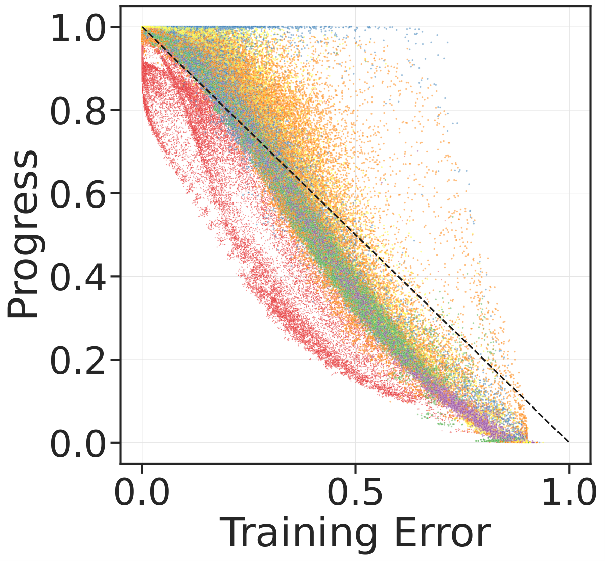
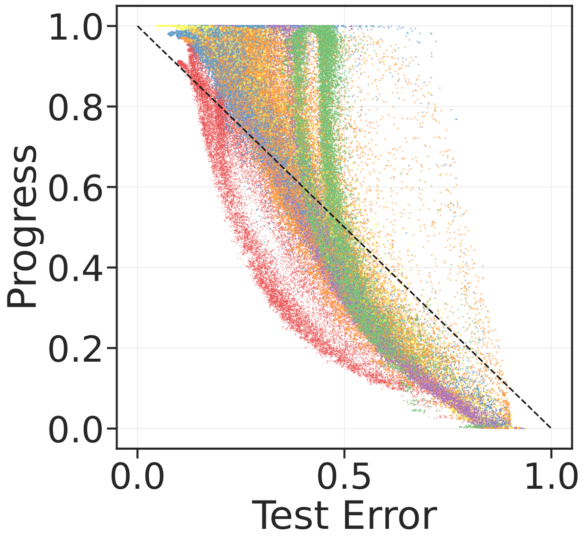
Networks with different configurations make progress towards the truth at different rates. As Fig. 8 shows, progress is strongly correlated with both train error () and test error (). Progress towards the train truth and towards the test truth are also highly correlated with each other (). This suggests that progress, which can be calculated easily using Eq. 4, is a good way to judge how close models are to both train and test truths. Note that models may not have a progress of 1 even if they have zero training error (AllCNN trained with Adam in our case). In our work, we have used progress, which is a geometrically natural quantity in probability space, to measure and interpolate trajectories. Fig. 8 also suggests that we could have used training error to interpolate checkpoints and would have obtained similar conclusions.
On both train and test manifold, at low error, AllCNN in red and Large ResNet in yellow have markedly different progress than other architectures (too low and too high respectively). Recall from Fig. 2(a) and Fig. 7(a) that trajectories of AllCNNs are also closest to the geodesic and those of Large ResNet are farthest. At high errors, which are typically seen at early training times, all architectures exhibit similar progress. Different weight initializations do not result in different rates of progress. For the same batch-size, SGD with Nesterov’s acceleration makes faster progress than SGD or Adam at very early training times but this difference vanishes at later stages of training. In general, models trained with weight decay achieve a lower final progress on both train and test manifolds.
We saw in Fig. 7(a) that trajectories of the Large ResNet lie on the same sub-manifold as that of the Small ResNet; see Fig. S.6 for the tube widths. The trend for the test manifold in Fig. 9(a) is similar. After the same number of gradient updates, the Large ResNet makes more progress towards the truth than the Small ResNet on CIFAR-10 (Fig. 9(a)). Fig. 9(b) shows the training progress against epochs averaged over different weight initializations for models trained on ImageNet. Again, the larger network (ResNet-50) makes more progress compared to the smaller network (ResNet-18) when trained using an identical optimization algorithm, learning rate schedule, batch-size and data augmentation.
Discussion
A new insight into optimization in deep learning
The central challenge in understanding why we can train deep networks effectively stems from the fact that the likelihood of an output given an input is a complicated function of the parameters . There is a large body of work that tackles this issue, e.g., optimization and generalization in function spaces for simpler architectures Baldi and Hornik 1989; Liang and Rakhlin 2020 or analytical models Mei et al. 2019; Chizat and Bach 2020; Jacot et al. 2018, analyzing representations of different layers Shwartz-Ziv and Tishby 2017; Achille and Soatto 2018, properties of stochastic optimization methods Chaudhari and Soatto 2018 etc. This has led to some successes, e.g., a characterization of the training dynamics and generalization for two-layer neural networks. But there is a vast diversity of different architectures, optimization methods and regularization mechanisms in deep learning, and it is difficult to draw general conclusions from these analyses.
We have taken a different approach in this experimental paper. We studied many different network configurations to discover surprising phenomena that are not predicted by existing theory. We give two examples here. First, the optimization process explores an effectively low-dimensional manifold in the space of predictions on the train and test data, in spite of the enormous dimensionality of both the embedding space and the weight space. This suggests that the optimization problem in deep learning might have a much smaller computational complexity than what is suggested by existing theory. Second, there is overwhelming empirical evidence that large networks with more parameters generalize better than smaller networks with fewer parameters Brown et al. 2020; Vaswani et al. 2017; Dosovitskiy et al. 2021. A large body of work has sought to analyze this phenomenon Belkin 2021; Belkin et al. 2019; Bartlett et al. 2021 and it has also been argued that we need to rethink our understanding of generalization in machine learning Zhang et al. 2017a. We have found that a Large ResNet trains along the same manifold as that of a Small ResNet. It proceeds further towards the truth in the later parts of the trajectory. In view of the effectiveness of pruning and knowledge distillation Frankle and Carbin 2019; Hinton et al. 2015, this could mean that the superior test error of large networks could be matched by smaller networks using better training methods.
There is some previous work that has argued that weight configurations along a particular training trajectory lie on low-dimensional manifolds, e.g., using PCA Feng and Tu 2021, or by arguing that the mini-batch gradient has a large overlap with the subspace spanned by the top few eigenvectors of the Hessian during training for networks without batch-normalization Gur-Ari et al. 2018; Ghorbani et al. 2019; Sagun et al. 2017. These analyses that study the low-dimensionality of trajectories in the weight space provide important insights into the dynamics of training and foreshadow our work. But their findings are not related to the ones we discussed here. To wit, weights of different architectures lie in totally different vector spaces. We also checked that weights along trajectories of the same network configuration but different weight initialization cannot be explained using few principal components, i.e., they do not lie in a low-dimensional linear subspace, and in fact the explained variance of the top few dimensions decreases proportionally with the number of distinct weight initializations. The mapping between the weight space and the prediction space is quite complicated, and phenomena that occur in the former do not imply that they occur in the latter space in general. Even if the set of models explored by the training process were to lie in a low-dimensional linear subspace, the set of predictions of these models need not lie in a low-dimensional linear subspace. This is because the singular vectors of the Jacobian between the prediction space and the weight space can rotate. Conversely, if the predictions of a set of models lie on low-dimensional manifolds, this does not imply that weights do so as well, because, for instance, there are symmetries in the the parameterization of deep networks.
Computational Information Geometry
Information Geometry Amari 2016 is a rich body of sophisticated ideas, but it has been difficult to wield it computationally, especially for high-dimensional probabilistic models like deep networks. The construction in Eq. 1 is a finite-dimensional probability distribution, in contrast to the standard object in information geometry which is an infinite-dimensional probability distribution defined over the entire domain of input data. It is this construction fundamentally that enables us to perform complicated computations such as, embeddings of high-dimensional models, geodesics in these spaces, projections of a model onto the geodesic, distances between trajectories in the prediction space, etc. Analysis of high-dimensional probabilistic models is challenging due to the curse of dimensionality: most points are orthogonal to each other in such spaces Antognini and Sohl-Dickstein 2018. Our visualization techniques, that build upon InPCA and IsKL Quinn et al. 2019; Teoh et al. 2020, work around this issue using multi-dimensional scaling Cox and Cox 2008; Saxe et al. 2019 and distances between probability distributions that violate the triangle inequality, e.g., the Bhattacharya distance. This has some mysterious benefits, e.g., our visualization technique can distinguish between small differences in high-dimensional probability distributions as they approach the truth in Minkowski space Laub and Müller 2004. Together with these visualization techniques, the theory developed in this paper gives new tools for the analysis of high-dimensional probabilistic models.
Interpretation of the top three principal coordinates
It is surprising that just three-dimensions can capture 76% of the stress (for CIFAR-10) of such a large set of diverse training trajectories in Fig. 2(a). We next offer an interpretation of this phenomenon. Our probabilistic models are an -product of probability distributions corresponding to points which lie on a -dimensional sphere. Training trajectories begin near ignorance and end near , so let us consider the straight line that joins ignorance and truth as one basis. Tangents to a training trajectory at ignorance (e.g., when networks are presumably learning “easy” images) and at truth (e.g., when networks are learning the most challenging images) can be two more basis vectors. This defines a three-dimensional subspace of the 450,000-dimensional prediction space. To represent this three-dimensional space, we can choose four probability distributions: , , and computed by weighted averages of models with progress close to and , respectively. The latter two are stand-ins for the tangents to the trajectories at and and they are calculated using
| (11) |
where is the normalizing factor and is the progress of the model . We choose for all the experiments and experiment with different choices of and . We can now build an InPCA embedding using these 4 models, and using the procedure in Eq. 9 (which is equivalent to weighted-InPCA discussed in Section D.3) we can add our original models in Fig. 2(a) into this new InPCA embedding.
Fig. 10 shows how well these new coordinates explain pairwise Bhattacharyya distances in for models of three configurations (AllCNN architectures trained with SGD, SGD with Nesterov’s acceleration and Adam) for ten different weight initializations by calculating
| (12) |
where are the -dimensional coordinates of the embedded points; we can calculate this quantity that we call “explained pairwise distances” using both these new and the original InPCA coordinates. Explained pairwise distances using the original InPCA embedding (which was created using all models) and this new InPCA embedding (which was created using only the 4 points: and for ) are both quite large—and similar to each other. The two embeddings are also consistent as to which coordinates are time-like (dimensions in Fig. 10 are ordered by the magnitude of eigenvalues).


We next performed the same analysis but with all models in Fig. 2(a) with , which effectively removes models that lie away from the manifold. In Fig. 11(a), we created an InPCA embedding using 4 points: ignorance , truth and for by computing the average over all models in Eq. 11, and projected the original probabilistic models into these new coordinates using the procedure in Eq. 9 to visualize them. We rotated the top 3 non-trivial dimensions of this embedding to best align the embedding created using the original InPCA procedure that uses all models to compute the embedding. This alignment was done using the Kabsh-Umeyama algorithm Lawrence et al. 2019 which finds the optimal translation, rotation and sign-flips of the coordinates to align two sets of points; the root mean square deviation (RMSD) is 0.06. As Fig. 11(b) shows, there are structural similarities in the embedding computed using only the 4 points and the one computed using all models, e.g., Small and Large ResNet models are close to those of ConvMixer models, and far from fully-connected models, some ResNets and ConvMixer models are away from the main manifold at intermediate training times. Fig. 11(c) shows that the new embedding also preserves pairwise Bhattacharyya distances between the models to a similar degree.
This exercise gives us an interpretation for the low-dimensional embedding discovered by InPCA. It may point to a mechanistic explanation for our findings: the train and test manifolds are effectively low-dimensional because networks with different architectures, optimization algorithms, hyper-parameter settings and regularization mechanisms fit the same easy images in the dataset first and the same challenging images towards the end of training; this phenomenon has also been studied in Hacohen et al. 2020.
Why are the train and test manifolds effectively low-dimensional?
It is remarkable that trajectories of networks with such different configurations lie on a manifold whose dimensionality is much smaller than the embedding dimension. To explore this further, we analyzed trajectories of networks trained on synthetic data: (a) sampled from a “sloppy” Gaussian, i.e., with eigenvalues of the covariance that are distributed uniformly on a logarithmic scale (this structure has been noticed in many typical problems Yang et al. 2022; Quinn et al. 2021), and (b) sampled from an isotropic Gaussian (non-sloppy data). We labeled these samples using a random two-layer fully-connected teacher network and trained student networks with different configurations to fit these labels. When students are initialized near ignorance , train and test manifolds are effectively low-dimensional for both kinds of data (87% explained stress in top ten dimensions). When students are initialized at different initial points similar to those in Fig. S.10, train and test manifolds are still effectively low-dimensional for both kinds of data; top ten dimensions have 85% explained stress. But the explained stress is higher in the top few dimensions if trajectories begin from near each other, e.g., from fewer initial points, or from ignorance. For sloppy input data, trajectories converge to the same manifold quickly even if they begin from very different initial points. Appendix F discusses this experiment further.
We therefore believe that the low-dimensionality of the manifold arises from (a) the structure of typical datasets Goldt et al. 2020; d’Ascoli et al. 2021; Refinetti et al. 2021, e.g., spectral properties, and (b) the fact that typical training procedures initialize models near one specific point in the prediction space, the ignorance . Along the first direction, recent work on understanding generalization Bartlett et al. 2020; Yang et al. 2022 has argued that deep networks, as also linear/kernel models, can interpolate without overfitting if input data have a sloppy spectrum. Work in neuroscience Simoncelli and Olshausen 2001; Field 1994 has also argued for visual data being effectively low-dimensional. Theories in machine learning Vapnik 1998; Schölkopf and Smola 2002 and information-theory Rissanen 1978; Balasubramanian 1997 for model selection are based on estimates of the number of models in a hypothesis class that are consistent with the data. In this context, our second suspect, namely initialization, suggests that even if the size of the hypothesis space might be very large for deep networks Dziugaite and Roy 2017; Bartlett et al. 2017, the subset of the hypothesis space explored by typical training algorithms might be much smaller.
Acknowledgments
JM, RR, RY and PC were supported by grants from the National Science Foundation (IIS-2145164, CCF-2212519), the Office of Naval Research (N00014-22-1-2255), and cloud computing credits from Amazon Web Services. IG was supported by the National Science Foundation (DMREF-89228, EFRI-1935252) and Eric and Wendy Schmidt AI in Science Postdoctoral Fellowship. HKT was supported by the National Institutes of Health (1R01NS116595-01). JPS was supported by the National Science Foundation (DMR-1719490), MKT was supported by the National Science Foundation (DMR-1753357). The authors would like to acknowledge Itai Cohen and Jay Spendlove for helpful comments on this material and manuscript.
References
- Teoh et al. (2020) Han Kheng Teoh, Katherine N. Quinn, Jaron Kent-Dobias, Colin B. Clement, Qingyang Xu, and James P. Sethna. Visualizing probabilistic models in Minkowski space with intensive symmetrized Kullback-Leibler embedding. Physical Review Research, 2(3):033221, August 2020. ISSN 2643-1564.
- Amari (2016) Shun-ichi Amari. Information Geometry and Its Applications, volume 194 of Applied Mathematical Sciences. Tokyo, 2016.
- Ito and Dechant (2020) Sosuke Ito and Andreas Dechant. Stochastic time evolution, information geometry, and the Cramér-Rao bound. Physical Review X, 10(2):021056, 2020.
- Brent (1971) Richard P. Brent. An algorithm with guaranteed convergence for finding a zero of a function. The computer journal, 14(4):422–425, 1971.
- Quinn et al. (2019) Katherine N Quinn, Colin B Clement, Francesco De Bernardis, Michael D Niemack, and James P Sethna. Visualizing probabilistic models and data with intensive principal component analysis. Proceedings of the National Academy of Sciences, 116(28):13762–13767, 2019.
- Cox and Cox (2008) Michael AA Cox and Trevor F Cox. Multidimensional scaling. In Handbook of Data Visualization, pages 315–347. 2008.
- Van der Maaten and Hinton (2008) Laurens Van der Maaten and Geoffrey Hinton. Visualizing data using t-SNE. Journal of machine learning research, 9(11), 2008.
- McInnes et al. (2018) Leland McInnes, John Healy, Nathaniel Saul, and Lukas Großberger. UMAP: Uniform manifold approximation and projection. Journal of Open Source Software, 3(29):861, 2018.
- De Silva and Tenenbaum (2004) Vin De Silva and Joshua B Tenenbaum. Sparse multidimensional scaling using landmark points. Technical report, Technical Report, Stanford University, 2004.
- Nielsen and Boltz (2011) Frank Nielsen and Sylvain Boltz. The burbea-rao and bhattacharyya centroids. IEEE Transactions on Information Theory, 57(8):5455–5466, 2011.
- Krizhevsky (2009) A. Krizhevsky. Learning Multiple Layers of Features from Tiny Images. PhD thesis, Computer Science, University of Toronto, 2009.
- Springenberg et al. (2015) Jost Tobias Springenberg, Alexey Dosovitskiy, Thomas Brox, and Martin Riedmiller. Striving for Simplicity: The All Convolutional Net. arXiv:1412.6806 [cs], April 2015.
- Zagoruyko and Komodakis (2016) Sergey Zagoruyko and Nikos Komodakis. Wide residual networks. In British Machine Vision Conference 2016, 2016.
- Trockman and Kolter (2022) Asher Trockman and J Zico Kolter. Patches are all you need? arXiv preprint arXiv:2201.09792, 2022.
- Dosovitskiy et al. (2020) Alexey Dosovitskiy, Lucas Beyer, Alexander Kolesnikov, Dirk Weissenborn, Xiaohua Zhai, Thomas Unterthiner, Mostafa Dehghani, Matthias Minderer, Georg Heigold, Sylvain Gelly, et al. An image is worth 16x16 words: Transformers for image recognition at scale. arXiv preprint arXiv:2010.11929, 2020.
- Kingma and Ba (2015) Diederik Kingma and Jimmy Ba. Adam: A method for stochastic optimization. In International Conference for Learning Representations, 2015.
- Ioffe and Szegedy (2015) Sergey Ioffe and Christian Szegedy. Batch normalization: Accelerating deep network training by reducing internal covariate shift. In International Conference on Machine Learning, pages 448–456, 2015.
- He et al. (2016) Kaiming He, Xiangyu Zhang, Shaoqing Ren, and Jian Sun. Deep residual learning for image recognition. In Proceedings of the IEEE Conference on Computer Vision and Pattern Recognition, pages 770–778, 2016.
- Heo et al. (2021) Byeongho Heo, Sanghyuk Chun, Seong Joon Oh, Dongyoon Han, Sangdoo Yun, Gyuwan Kim, Youngjung Uh, and Jung-Woo Ha. Adamp: Slowing down the slowdown for momentum optimizers on scale-invariant weights. In International Conference on Learning Representations (ICLR), 2021.
- Transtrum et al. (2011) Mark K. Transtrum, Benjamin B. Machta, and James P. Sethna. The geometry of nonlinear least squares with applications to sloppy models and optimization. Physical Review E, 83(3):036701, March 2011. ISSN 1539-3755, 1550-2376.
- Amari (1998) Shun-ichi Amari. Natural gradient works efficiently in learning. Neural Computation, 10(2):251–276, 1998.
- Baldi and Hornik (1989) P. Baldi and K. Hornik. Neural networks and principal component analysis: Learning from examples without local minima. Neural Networks, 2:53–58, 1989.
- Liang and Rakhlin (2020) Tengyuan Liang and Alexander Rakhlin. Just interpolate: Kernel “ridgeless” regression can generalize. The Annals of Statistics, 48(3):1329–1347, 2020.
- Mei et al. (2019) Song Mei, Theodor Misiakiewicz, and Andrea Montanari. Mean-field theory of two-layers neural networks: Dimension-free bounds and kernel limit. In Conference on Learning Theory, pages 2388–2464, 2019.
- Chizat and Bach (2020) Lenaic Chizat and Francis Bach. Implicit bias of gradient descent for wide two-layer neural networks trained with the logistic loss. In Conference on Learning Theory, pages 1305–1338, 2020.
- Jacot et al. (2018) Arthur Jacot, Franck Gabriel, and Clement Hongler. Neural tangent kernel: Convergence and generalization in neural networks. In Advances in Neural Information Processing Systems 31, pages 8571–8580. 2018.
- Shwartz-Ziv and Tishby (2017) Ravid Shwartz-Ziv and Naftali Tishby. Opening the Black Box of Deep Neural Networks via Information. arXiv:1703.00810 [cs], April 2017.
- Achille and Soatto (2018) Alessandro Achille and Stefano Soatto. Emergence of invariance and disentanglement in deep representations. The Journal of Machine Learning Research, 19(1):1947–1980, 2018.
- Chaudhari and Soatto (2018) Pratik Chaudhari and Stefano Soatto. Stochastic gradient descent performs variational inference, converges to limit cycles for deep networks. In Proc. of International Conference of Learning and Representations (ICLR), 2018.
- Brown et al. (2020) Tom Brown, Benjamin Mann, Nick Ryder, Melanie Subbiah, Jared D Kaplan, Prafulla Dhariwal, Arvind Neelakantan, Pranav Shyam, Girish Sastry, Amanda Askell, et al. Language models are few-shot learners. Advances in neural information processing systems, 33:1877–1901, 2020.
- Vaswani et al. (2017) Ashish Vaswani, Noam Shazeer, Niki Parmar, Jakob Uszkoreit, Llion Jones, Aidan N Gomez, Lukasz Kaiser, and Illia Polosukhin. Attention is all you need. In Advances in Neural Information Processing Systems, 2017.
- Dosovitskiy et al. (2021) Alexey Dosovitskiy, Lucas Beyer, Alexander Kolesnikov, Dirk Weissenborn, Xiaohua Zhai, Thomas Unterthiner, Mostafa Dehghani, Matthias Minderer, Georg Heigold, Sylvain Gelly, Jakob Uszkoreit, and Neil Houlsby. An image is worth 16x16 words: Transformers for image recognition at scale. In International Conference on Learning Representations, 2021.
- Belkin (2021) Mikhail Belkin. Fit without fear: Remarkable mathematical phenomena of deep learning through the prism of interpolation. arXiv preprint arXiv:2105.14368, 2021.
- Belkin et al. (2019) Mikhail Belkin, Daniel Hsu, Siyuan Ma, and Soumik Mandal. Reconciling modern machine-learning practice and the classical bias–variance trade-off. Proceedings of the National Academy of Sciences, 116(32):15849–15854, 2019.
- Bartlett et al. (2021) Peter L. Bartlett, Andrea Montanari, and Alexander Rakhlin. Deep learning: A statistical viewpoint. Acta Numerica, 30:87–201, 2021.
- Zhang et al. (2017a) Chiyuan Zhang, Samy Bengio, Moritz Hardt, Benjamin Recht, and Oriol Vinyals. Understanding deep learning requires rethinking generalization. In International Conference on Learning Representations (ICLR), 2017a.
- Frankle and Carbin (2019) Jonathan Frankle and Michael Carbin. The Lottery Ticket Hypothesis: Finding Sparse, Trainable Neural Networks. arXiv:1803.03635 [cs], March 2019.
- Hinton et al. (2015) Geoffrey Hinton, Oriol Vinyals, and Jeff Dean. Distilling the knowledge in a neural network. NIPS Deep Learning and Representation Learning Workshop, 2015.
- Feng and Tu (2021) Yu Feng and Yuhai Tu. The inverse variance–flatness relation in stochastic gradient descent is critical for finding flat minima. Proceedings of the National Academy of Sciences, 118(9):e2015617118, Mar 2021. 10.1073/pnas.2015617118.
- Gur-Ari et al. (2018) Guy Gur-Ari, Daniel A. Roberts, and Ethan Dyer. Gradient descent happens in a tiny subspace. (arXiv:1812.04754), Dec 2018. URL http://arxiv.org/abs/1812.04754. arXiv:1812.04754 [cs, stat].
- Ghorbani et al. (2019) Behrooz Ghorbani, Shankar Krishnan, and Ying Xiao. An investigation into neural net optimization via hessian eigenvalue density. In Proceedings of the 36th International Conference on Machine Learning, 2019.
- Sagun et al. (2017) Levent Sagun, Leon Bottou, and Yann LeCun. Eigenvalues of the hessian in deep learning: Singularity and beyond. (arXiv:1611.07476), Oct 2017. 10.48550/arXiv.1611.07476. URL http://arxiv.org/abs/1611.07476. arXiv:1611.07476 [cs].
- Antognini and Sohl-Dickstein (2018) Joseph Antognini and Jascha Sohl-Dickstein. PCA of high dimensional random walks with comparison to neural network training. Advances in Neural Information Processing Systems, 31, 2018.
- Saxe et al. (2019) Andrew M Saxe, James L McClelland, and Surya Ganguli. A mathematical theory of semantic development in deep neural networks. Proceedings of the National Academy of Sciences, 116(23):11537–11546, 2019.
- Laub and Müller (2004) Julian Laub and Klaus-Robert Müller. Feature discovery in non-metric pairwise data. The Journal of Machine Learning Research, 5:801–818, 2004.
- Lawrence et al. (2019) Jim Lawrence, Javier Bernal, and Christoph Witzgall. A purely algebraic justification of the Kabsch-Umeyama algorithm. Journal of research of the National Institute of Standards and Technology, 124:1, 2019.
- Hacohen et al. (2020) Guy Hacohen, Leshem Choshen, and Daphna Weinshall. Let’s agree to agree: Neural networks share classification order on real datasets. In International Conference on Machine Learning, pages 3950–3960, 2020.
- Yang et al. (2022) Rubing Yang, Jialin Mao, and Pratik Chaudhari. Does the data induce capacity control in deep learning? In Proc. of International Conference of Machine Learning (ICML), 2022.
- Quinn et al. (2021) Katherine N. Quinn, Michael C. Abbott, Mark K. Transtrum, Benjamin B. Machta, and James P. Sethna. Information geometry for multiparameter models: New perspectives on the origin of simplicity. page arXiv:2111.07176, 2021.
- Goldt et al. (2020) Sebastian Goldt, Marc Mézard, Florent Krzakala, and Lenka Zdeborová. Modeling the influence of data structure on learning in neural networks: The hidden manifold model. Physical Review X, 10(4):041044, 2020.
- d’Ascoli et al. (2021) Stéphane d’Ascoli, Marylou Gabrié, Levent Sagun, and Giulio Biroli. On the interplay between data structure and loss function in classification problems. Advances in Neural Information Processing Systems, 34:8506–8517, 2021.
- Refinetti et al. (2021) Maria Refinetti, Sebastian Goldt, Florent Krzakala, and Lenka Zdeborová. Classifying high-dimensional gaussian mixtures: Where kernel methods fail and neural networks succeed. In International Conference on Machine Learning, pages 8936–8947, 2021.
- Bartlett et al. (2020) Peter L Bartlett, Philip M Long, Gábor Lugosi, and Alexander Tsigler. Benign overfitting in linear regression. Proceedings of the National Academy of Sciences, 117(48):30063–30070, 2020.
- Simoncelli and Olshausen (2001) Eero P Simoncelli and Bruno A Olshausen. Natural image statistics and neural representation. Annual review of neuroscience, 24(1):1193–1216, 2001.
- Field (1994) David J Field. What is the goal of sensory coding? Neural computation, 6(4):559–601, 1994.
- Vapnik (1998) Vladimir Vapnik. Statistical Learning Theory. 1998.
- Schölkopf and Smola (2002) Bernhard Schölkopf and Alexander J Smola. Learning with Kernels. 2002.
- Rissanen (1978) Jorma Rissanen. Modeling by shortest data description. Automatica, 14(5):465–471, 1978.
- Balasubramanian (1997) Vijay Balasubramanian. Statistical Inference, Occam’s Razor, and Statistical Mechanics on the Space of Probability Distributions. Neural Computation, 9(2):349–368, February 1997. ISSN 0899-7667, 1530-888X.
- Dziugaite and Roy (2017) Gintare Karolina Dziugaite and Daniel M. Roy. Computing Nonvacuous Generalization Bounds for Deep (Stochastic) Neural Networks with Many More Parameters than Training Data. In Proc. of the Conference on Uncertainty in Artificial Intelligence (UAI), 2017.
- Bartlett et al. (2017) Peter L Bartlett, Dylan J Foster, and Matus J Telgarsky. Spectrally-normalized margin bounds for neural networks. In Advances in Neural Information Processing Systems, pages 6240–6249, 2017.
- Bishop et al. (1995) Christopher M Bishop et al. Neural Networks for Pattern Recognition. 1995.
- Krizhevsky et al. (2012) Alex Krizhevsky, Ilya Sutskever, and Geoffrey E Hinton. Imagenet classification with deep convolutional neural networks. In Advances in Neural Information Processing Systems, pages 1097–1105, 2012.
- Deng et al. (2009) Jia Deng, Wei Dong, Richard Socher, Li-Jia Li, Kai Li, and Li Fei-Fei. Imagenet: A large-scale hierarchical image database. In 2009 IEEE Conference on Computer Vision and Pattern Recognition, pages 248–255, 2009.
- Srivastava et al. (2014) Nitish Srivastava, Geoffrey Hinton, Alex Krizhevsky, Ilya Sutskever, and Ruslan Salakhutdinov. Dropout: A simple way to prevent neural networks from overfitting. JMLR, 15(1):1929–1958, 2014.
- Ba et al. (2016) Jimmy Lei Ba, Jamie Ryan Kiros, and Geoffrey E. Hinton. Layer Normalization. arXiv:1607.06450 [cs, stat], July 2016.
- Zhang (2019) Richard Zhang. Making convolutional networks shift-invariant again. In International conference on machine learning, pages 7324–7334. PMLR, 2019.
- Touvron et al. (2021) Hugo Touvron, Matthieu Cord, Matthijs Douze, Francisco Massa, Alexandre Sablayrolles, and Hervé Jégou. Training data-efficient image transformers & distillation through attention. In International conference on machine learning, pages 10347–10357. PMLR, 2021.
- Leclerc et al. (2022) Guillaume Leclerc, Andrew Ilyas, Logan Engstrom, Sung Min Park, Hadi Salman, and Aleksander Madry. ffcv. https://github.com/libffcv/ffcv/, 2022.
- Wightman (2019) Ross Wightman. Pytorch image models. https://github.com/rwightman/pytorch-image-models, 2019.
- Goyal et al. (2017) Priya Goyal, Piotr Dollár, Ross Girshick, Pieter Noordhuis, Lukasz Wesolowski, Aapo Kyrola, Andrew Tulloch, Yangqing Jia, and Kaiming He. Accurate, large minibatch SGD: Training ImageNet in 1 hour. arXiv:1706.02677, 2017.
- He et al. (2019) Tong He, Zhi Zhang, Hang Zhang, Zhongyue Zhang, Junyuan Xie, and Mu Li. Bag of tricks for image classification with convolutional neural networks. In Proceedings of the IEEE Conference on Computer Vision and Pattern Recognition, pages 558–567, 2019.
- Zhang et al. (2017b) Hongyi Zhang, Moustapha Cisse, Yann N Dauphin, and David Lopez-Paz. mixup: Beyond empirical risk minimization. arXiv preprint arXiv:1710.09412, 2017b.
- Dhillon et al. (2020) Guneet S Dhillon, Pratik Chaudhari, Avinash Ravichandran, and Stefano Soatto. A baseline for few-shot image classification. In Proc. of International Conference of Learning and Representations (ICLR), 2020.
- Thrun and Pratt (2012) Sebastian Thrun and Lorien Pratt. Learning to Learn. 2012.
- Vo et al. (2008) Nhat Vo, Duc Vo, SungYoung Lee, and Subhash Challa. Weighted nonmetric MDS for sensor localization. In 2008 International Conference on Advanced Technologies for Communications, pages 391–394. IEEE, 2008.
- Gabriel and Zamir (1979) K Ruben Gabriel and Shmuel Zamir. Lower rank approximation of matrices by least squares with any choice of weights. Technometrics, 21(4):489–498, 1979.
- Greenacre (2005) Michael Greenacre. Weighted metric multidimensional scaling. In New Developments in Classification and Data Analysis: Proceedings of the Meeting of the Classification and Data Analysis Group (CLADAG) of the Italian Statistical Society, University of Bologna, September 22–24, 2003, pages 141–149. Springer, 2005.
- Delchambre (2015) Ludovic Delchambre. Weighted principal component analysis: a weighted covariance eigendecomposition approach. Monthly Notices of the Royal Astronomical Society, 446(4):3545–3555, 2015.
- Nielsen (2013) Frank Nielsen. Jeffreys centroids: A closed-form expression for positive histograms and a guaranteed tight approximation for frequency histograms. IEEE Signal Processing Letters, 20(7):657–660, 2013.
Appendix A Notation
| Symbol | Description |
|---|---|
| Number of samples | |
| Number of classes | |
| Input sample with index | |
| Label assignment of sample with index | |
| Ground-truth label of sample with index | |
| Weights of the deep network | |
| Ground-truth labels for each of the samples, | |
| Label assignment for each of the samples, | |
| Probability that sample belongs to class , | |
| Probabilistic model with weight ; assigns a probability to every sequence | |
| Truth () | |
| Ignorance, has for all classes and samples | |
| Bhattacharyya distance between two probability distributions | |
| Geodesic distance (great circle distance) between two probability distributions | |
| Fisher Information Metric (FIM) at weight configuration | |
| Point on a -dimensional sphere | |
| Geodesic between probability distributions and parameterized by | |
| Number of recorded checkpoints | |
| A sequence of recorded checkpoints in the weight space | |
| Progress of a probabilistic model with weights | |
| Interpolating parameter along a geodesic, | |
| A sequence of probabilistic models recorded during training, also denoted by | |
| A continuous curve in the space of probabilistic models, also denoted by | |
| Distance between trajectories and | |
| Matrix () of pairwise Bhattacharyya distances between probabilistic models, entries of this matrix are denoted by etc. depending upon the context | |
| Matrix () of centered pairwise Bhattacharyya distances, where performs the centering | |
| Coordinates () of the InPCA embedding of a model with weights | |
| Explained stress, used to estimate the fraction of the entries of the centered pairwise distance matrix that are preserved by an embedding; equivalent to explained variances in standard PCA (up to the square root) | |
| Explained pairwise distances, used to estimate the fraction of the entries of the pairwise Bhattacharyya distance matrix that are preserved by an embedding |
Appendix B Derivation of the joint probability of predictions and the Bhattacharyya distance
The quantity in Eq. 1 is the joint likelihood of all the labels given the weights. Observe that
In this calculation, we have used the assumption that (a) predictions on two samples are independent of each other given the weights and the input samples (if we marginalize on the weights, they are certainly dependent), (b) we are performing inductive inference, i.e., , and (c) the samples are frozen to the ones in the training set for the analysis, i.e., the distribution . So we actually do not need to use the assumption that the training samples are independent of each other to write down the joint likelihood that factorizes over the samples in the training set. Certainly, if the training samples are independent, then this derivation also holds. Let us note that training samples being independent of each other is one of the most common assumptions in machine learning. This assumption is used to derive, for instance, the maximum likelihood estimator in (Bishop et al. 1995, Equation 1.61).
The expression for the Bhattacharyya distance between two probability distributions and in Eq. 2 can be derived as follows. Note that can take a total of distinct values, and each .
Calculations like the one above hold in general, the joint entropy of two independent random variables is the sum of their individual entropy. Just like the familiar cross-entropy loss used for training deep networks is an average over the samples, the Bhattacharyya distance is also an average over the training samples.
Appendix C Details of the experimental setup
Datasets
The experimental data in this paper was obtained by training deep networks on two datasets.
- •
The CIFAR-10 dataset Krizhevsky et al. 2012 has RGB images in the training set of size 32 32 from different categories (airplane, automobile, bird, cat, deer, dog, frog, horse, ship and truck). The test set has images. Both train and test sets have an equal number of images in each category.
- •
The ImageNet dataset Deng et al. 2009 has categories and a total of RGB images of size 224 224 in the training dataset. Different categories have slightly different numbers of images in the train set, but all categories have at least 1000 images. The test set consists of images, with 50 images from each category.
Neural architectures
For CIFAR-10, we used six neural architectures. These architectures were chosen and and configurations were chosen to ensure that these networks could fit all the images in the training dataset, i.e., achieve zero training error, for most training methods.
- 1.
A multi-layer perceptron with rectified linear unit (ReLU) nonlinearities (fully-connected network) with 4 hidden layers, of size [1024, 512, 256, 128] respectively.
- 2.
An “all convolutional network” (AllCNN Springenberg et al. 2015) with 5 convolutional layers followed by an average pooling layer; first three layers have 96 channels and the latter two have 144 channels.
- 3.
Two different wide residual networks Zagoruyko and Komodakis 2016. The larger one has 16 layers and [64, 256, 1024, 4096] channels for the convolutional layers in the four blocks, and the smaller network has 10 layers with [8, 32, 128, 512] channels for the four blocks. Both networks have a “widening factor” of 4. We modified the implementation at https://github.com/meliketoy/wide-resnet.pytorch.
- 4.
The ConvMixer architecture Trockman and Kolter 2022 is a convolutional network but it uses very large receptive fields and maintains the same size for the activations across successive layers. We did not make any changes to the architecture from the original paper.
- 5.
The ViT architecture Dosovitskiy et al. 2021 is a self-attention based network that uses a set of disjoint patches of size 44 from the input images. This network does not use convolutional operations and instead uses the so-called self-attention layer that is popularly in natural language processing. We use a linear layer size of 512, 8 self-attention heads and 6 transformer blocks (layers). We used the implementation from https://github.com/lucidrains/vit-pytorch.
We do not use Dropout Srivastava et al. 2014 in any of the networks. All networks except ViT have a batch-normalization Ioffe and Szegedy 2015 layer after each convolutional or fully-connected layer, except ViT which uses layer normalization Ba et al. 2016.
For ImageNet, we used three architectures.
- 1.
A smaller residual network He et al. 2016 with 18 layers (ResNet-18). This residual network is different from the wide residual network used for CIFAR-10, primarily in that there are fewer channels in each block. A ResNet is architecturally similar to a wide residual network with a widening factor of 1. We replaced each strided convolution with a convolution followed by a BlurPool layer (Zhang 2019).
- 2.
A larger residual network with 50 layers (ResNet-50). This is one of the most popular networks for training on ImageNet and widely used as a benchmark architecture in the field.
- 3.
The ViT architecture which is similar to the one used for CIFAR-10 above except that the receptive field of the first layer is larger due to the larger images in ImageNet. We trained a smaller variant of ViT called ViT-S (with 22 million weights) which was introduced in (Touvron et al. 2021). It operates on patches of size 16 16 and has 6 self-attention heads and 12 transformer blocks.
Training multiple models on ImageNet is computationally expensive. To mitigate this, we used efficient data loaders, computed gradients in half-precision, and chose effective training hyper-parameters (FFCV (Leclerc et al. 2022) for training ResNets and timm (Wightman 2019) for training ViTs).
Training procedure
For both datasets, we normalize images in the train and test sets by the channel-wise mean and variance of the images in the training dataset. For CIFAR-10, we also augmented training images by randomly cropping a region of size 32 32 after padding the original image by 4 pixels on each side, and performing horizontal flips with a probability of 0.5; our data contains models trained with and without such data augmentation.
All the networks are initialized using the default PyTorch weight initialization as follows. For fully-connected layers with an input dimension , all weights and biases are sampled independently from a uniform distribution on . For convolutional layers with channels and a convolutional kernel, all weights and biases are sampled independently from a uniform distribution on .
We started with 3120 different configurations, 520 for each network architecture. Some networks did not finish training due to numerical errors during gradient updates, and we excluded them from our analysis. Fig. S.1 shows how many of the configurations did not finish training for each network architecture. Our data, with 2,296 different configurations, therefore contains fewer ViTs and Large ResNets than other architectures.
For CIFAR-10, we used three different optimization methods, stochastic gradient descent (SGD), SGD with Nesterov’s momentum (with a coefficient of 0.9) and Adam Kingma and Ba 2015, three different batch sizes (200, 500 and 1000) and three different values of the weight decay coefficient ( regularization) ( when training with SGD and SGD with Nesterov’s momentum, and when training with Adam). Fully-connected networks trained on augmented data are trained for 300 epochs to achieve zero training error, all other networks are trained for 200 epochs. One epoch corresponds to using each sample in the training dataset exactly once to compute a gradient update (i.e., mini-batches are sampled without replacement). As the batch-size in SGD is increased, the stochasticity of the weight updates decreases and this makes the iterations more susceptible to converging near local minima of the loss function, and thereby obtain poor test error. It has been noticed empirically that keeping the ratio of the learning rate to batch-size invariant helps mitigate this deterioration of test error for large batch sizes Goyal et al. 2017. This has also been argued theoretically via an analysis of the equilibrium distribution of SGD Chaudhari and Soatto 2018. Therefore, for SGD and SGD with Nesterov’s acceleration, we fixed this ratio to , i.e., for a batch size 200, we use a learning rate of 0.1, and increase the learning rate proportionally for larger batch sizes. For Adam, this ratio was , i.e., we used a learning rate of 0.001 for a batch-size of 200. For all experiments, we decreased the learning rate using a cosine annealing schedule over the course of training, i.e., for all networks the learning rate decays to zero at the end of training.
Residual networks on ImageNet were trained using SGD with Nesterov’s acceleration for 40 epochs with a batch-size of 1024. The learning rate was decreased linearly from 0.5. We used a weight decay coefficient of ; no weight decay was applied to parameters associated with batch-normalization. To reduce the training time, we used mixed-precision training. We also used progressive resizing, i.e., we trained on images of size 196 196 for the first 34 epochs before using the full-sized images (224 224) for the remaining 6 epochs. We use random horizontal flips and random-resize-crops for data augmentations. For datasets with a large number of classes such as ImageNet, it helps to use label smoothing He et al. 2019, we used this with the smoothing parameter set of 0.9. This amounts to training towards a slightly different truth where the correct category has a probability of 0.9 and the remainder 0.1 is distributed uniformly across the other 999 categories (instead of them being zero).
ViT architectures are difficult to train well with SGD, especially on large datasets such as ImageNet. We therefore trained ViTs on ImageNet using AdamP (Heo et al. 2021) with a cosine-annealed learning rate schedule and an initial learning rate of 0.001. We trained for 200 epochs using a batch-size of 1024 and weight decay of 0.01 without any dropout. These networks also require a more extensive set of data augmentations, we used horizontal flips with probability 0.5, cropping the image to get a patch of the desired size at a random location (images in ImageNet are not of the same size), and mixup regularization (Zhang et al. 2017b) which uses mini-batches that consist of convex combinations (with a random parameter) of images and ground-truth probability distributions.
Some ImageNet models are not initialized near ignorance
We noticed that some randomly initialized models have a large Bhattacharyya distance from ignorance . For example, the distance between a randomly initialized ResNet-50 model and ignorance is as much as 0.91 times the Bhattacharyya distance between ignorance and truth . We found that this is due to the batch-normalization layer (Ioffe and Szegedy 2015) being incorrectly initialized at the beginning of training. Batch-normalization subtracts the channel-wise mean of the activations (computed from samples in a mini-batch) and divides the result by an estimate of the channel-wise standard deviation of the activations (computed using the samples in the mini-batch). During training, typical deep learning libraries such as PyTorch maintain an exponentially moving average of the mean and standard deviation of activations of mini-batches. And it is these averaged estimates that are used to compute the output probabilities for test data. In PyTorch, the mean is initialized to zero and the standard deviation is initialized to 1. This causes the magnitude of the activations to be very large in the final few layers at initialization and that is why the probabilistic model is very far from ignorance at initialization, as shown in Fig. S.2.
This phenomenon is seen in most popular off-the-shelf implementations of a ResNet, and could also be present in other architectures. When training in a supervised learning setting, this finding of ours is only marginally relevant because the estimates of the mean and standard deviation stabilize to reasonable values within 5–10 mini-batch updates. But there are many sub-fields of machine learning, few-shot learning Dhillon et al. 2020, meta-learning Thrun and Pratt 2012 to name some, where the number of mini-batch updates of a trained model is a key parameter and where our finding has practical relevance. To fix this issue, we can initialize the batch-normalization mean and variance estimates—easily—by doing a forward pass on a few mini-batches from the training data before beginning the training. This ensures that the model starts training from near ignorance. When we collected data from our training trajectories on ImageNet, we did not have this fix. We therefore did not plot the first checkpoint for the ImageNet experiments in Figs. 2(d) and 5(d).
Appendix D Addendum to Methods
D.1 InPCA creates an isometric embedding
InPCA, like standard PCA, relies on an embedding directed by the centered pairwise distances Eq. 6. Observe that the centering in Eq. 6 is the same as the centering performed in standard PCA, indeed it ensures that rows and columns of the pairwise distance matrix sum to zero. Since InPCA involves pairwise Bhattacharyya distances, not pairwise Euclidean distances, such a centering is not trivially equivalent to a translation of points in a vector space. We show next that the embedding created using InPCA is isometric, i.e., it satisfies Eq. 7. The argument developed below also holds for other embedding techniques, e.g., the IsKL method discussed in Eq. 15 that uses the symmetrized Kullback-Leibler divergence as the distance between probability distributions.
Given a real symmetric matrix , we can write where the eigenvalues and columns of are the eigenvectors. We can define an “eigen-embedding” of such a matrix:
and a quasi inner-product for , with metric signature derived from the positive eigenvalues of . The quasi inner-product of the points in an eigen-embedding of a real symmetric matrix allows us to reconstruct the entries of :
| (13) |
Now consider a finite symmetric premetric space with points77 7 A premetric space satisfies two properties: that the distance between two points is non-negative, and the distance of a point from itself is zero.. If is a matrix of pairwise distances between these points, then it has a vanishing diagonal. The embedding of denoted by satisfies for any . Now observe that the distance between any and is the squared Minkowski interval between them, i.e.,
| (14) |
In other words, the points in can be isometrically embedded in a Minkowski space as the eigen-embedding of . The centering operation using a matrix which we use to compute ensures that
where is the mean of the eigen-embedding of ; in other words, the centered pairwise distance matrix is equal to the cross-covariance matrix in a Minkowski space.
Theorem 1.
Given a finite symmetric premetric space with points, if is the matrix of pairwise distances between these points, then the eigen-embedding of where is the centering matrix, is isometric to .
Proof.
Let the eigen-embeddings of and be and respectively. We know that the eigen-embedding of is isometric to . From Eq. 13, we have that and so . Since the centered pairwise distance matrix is equal to the cross-covariance matrix, we also have and therefore
∎
D.2 Relationship between progress and error
Progress is related to the error but they are not the same. Suppose we have a model that predicts very confidently, i.e., for all and all samples . The progress of this model is given by
where is the fraction of errors made by the model on the samples and if there are classes. We can show that if , then the progress . This suggests that progress and error are not directly analogous to each other: models with high progress do not necessarily have small errors. In practice, if the number of samples is small and the number of classes is large, then we will find instances of models with high progress and high error. This is not often the case in our experiments for the training data, but we do see very high progress for some models on the test data (see Fig. 8).
D.3 Emphasizing different models using a weighted embedding
To study the details of the model manifold, we have found it useful to emphasize certain models in the visualization. There are many works Vo et al. 2008; Gabriel and Zamir 1979; Greenacre 2005; Delchambre 2015 that do similar things, e.g., those that modify the underlying objective of MDS to optimize a weighted Euclidean distance (but this does not do a good job of preserving pairwise distances between points), or those that learn a set of orthogonal transformations to highlight points of interest. We can also repeat models while computing InPCA: this shifts the center of mass and,at the same time transforms the visualization (via rotations and Lorentz boosts). It emphasizes the repeated models in the visualization. However, such a naive approach is computationally expensive because the size of the distance matrix increases due to these repetitions.
We present a different approach called weighted-InPCA next. Let be the matrix of pairwise Bhattacharyya distances and let be multiplicity of the model with weights , i.e., the relative importance that we would like for it in the visualization. The normalized multiplicities are . Weighted-InPCA is a modification of InPCA. It (a) uses a different centering matrix , (b) performs an eigen-decomposition of , i.e., each column of is multiplied by , and (c) then scales back each of the eigenvectors using the expression . This procedure gives the same embedding as the one obtained by repeating points before calculating standard InPCA and is also equivalent to the procedure in Eq. 9 when the weights of the new points are zero.


D.4 Computing pairwise distances in InPCA using only a subset of the samples gives a faithful representation of the train and test manifolds
We computed the InPCA coordinates using a subset of the samples in the train and test sets to calculate the pairwise Bhattacharyya distance matrix. Using the procedure in Eq. 9, we then embedded the models in the original pairwise distance matrix computed using all samples into these InPCA coordinates. Figs. S.3 and S.4 show that the explained pairwise distances by the top three dimensions of these new InPCA embeddings is quite high. This suggests that our visualization methods could be used effectively, even for large datasets with a large number of samples , by sub-sampling the data before computing InPCA.
Appendix E Addendum to Results
E.1 Further analysis of the train trajectories
Understanding the differences between the trajectories of different configurations
Using the interpolated trajectories, for each configuration, we calculated the Euclidean mean of the probabilities of the models corresponding to different weight initializations at the same progress. The distance of the model to such a configuration-specific mean model gives us an understanding of the “tube width”, i.e., how different in prediction space models with the same progress but corresponding to different weight initializations are. Fig. 6(a) shows that—for all configurations, for all values of progress—models are very close to their respective mean model. The median tube width is about 0.05 in terms of Bhattacharyya distance throughout training; this should be compared to the abscissae of Fig. 7(a) where a cut at a distance of 0.05 separates all configurations (except some AllCNNs, and very few fully-connected and ConvMixer architectures). The dendrogram in Fig. 7(a) averages models for the same progress; Figs. 6(a) and 6(b) indicate that such averaging is a reasonable thing to do. The test manifold in Fig. 6(b) is similar, except that tube widths increase slightly with progress. This suggests that networks with different weight initializations train along very similar trajectories in prediction space.
One can dig deeper into the differences in models caused by weight initialization. Tube widths of different architectures at the same progress are similar on the train manifold, but there are more pronounced differences on the test manifold. We have found that variations coming from optimization methods and regularization do not result in large tube widths. In general, towards the end of training, at large values of progress, models trained with augmentation have larger tube widths than models trained without augmentation, on both train and test manifolds (Fig. S.5). Training a deep network is a non-convex optimization problem, and as such the solution depends upon the initialization of weights in a non-trivial way. Each point in the prediction space corresponds to a large set of weight configurations that lead to this same prediction. Our results therefore suggest that, even if different weight initializations could lead to different eventual weights for these non-convex optimization problems, the probabilistic models obtained at the end of training are very similar (they are more similar on the training data than the test data).


We next study the distances of models along the interpolated trajectories to the geodesic. On the train manifold (Fig. 7(a)), all models are very close to the geodesic at the beginning (small progress) and at the end of training (large progress). At intermediate progress, all trajectories have large distances to the geodesic; as we discussed above this deviation away from the geodesic could be an indicator of the range of difficulties of learning different samples. Trajectories corresponding to different architectures and optimization methods are at different distances from the geodesic at intermediate progress. Train trajectories of AllCNN are closest to the geodesic; there are marked differences between the three optimization algorithms in this case. But this is not so for other architectures. For test trajectories (Fig. 7(b)), the distance to the geodesic is roughly the same, and larger that that of the train manifold, for all architectures and all values of progress. At large progress, test trajectories of fully-connected and ViT networks are very far from the geodesic; this is also visible in Fig. 5.
Models initialized at very different parts of the prediction space converge to the truth along a similar manifold
The manifold in our analysis is the set of probabilistic models explored during the training process; this is a subset of the space of all probabilistic models (which is the simplex in and not low-dimensional). Our manifold is a subset of the manifold of all probabilistic models that can be expressed by the network (which is also not expected to be low-dimensional) because the training process does not explore all parts of the weight space. To understand why our trajectories seem to lie on effectively low-dimensional manifolds, using CIFAR-10, we created three different tasks by randomly assigning labels to the images, e.g., each image of a dog is labeled independently as any of the 10 possible classes. This gives us three random initial models denoted by for , and we can now train networks to fit these random labels. Both train and test manifolds of training to such random tasks are effectively low-dimensional. This suggests that the low-dimensionality is not necessarily due to there being learnable patterns in the labels.


We next performed a second stage of training where networks were initialized to the endpoints of the trajectories to for (models do not reach these points exactly during training), and trained on the actual CIFAR-10 task, i.e., to the actual truth . In this case, we only trained one particular configuration (AllCNN architecture, SGD without Nesterov’s acceleration, no augmentation or weight-decay) from 10 different weight initializations chosen to be near . This two-stage training procedure also results in effectively low-dimensional train and test manifolds (Figs. 10(a) and S.11); the top three dimensions explain more than 87% of the stress. It is interesting to note that the networks don’t just forget the wrong labels before learning the correct ones, trajectories rejoin the original training trajectory at a variety of points before following it to the truth.
In Fig. 10(b) we show the training trajectories to (light red) and from (red) , together with the geodesics connecting , and . The geodesic from to the truth does not pass near ignorance . In fact, a random task agrees with the truth on approximately of the samples, and the Bhattacharyya distance of the geodesic from to the truth is at least a distance ( for ) from ignorance. As a reference, the distance between training trajectories of two different configurations is about 0.15 in Fig. 7(a). Unlike the geodesic from , trajectories from come much closer to ignorance; the smallest distance from ranges from 0.1–0.5 for different weight initializations. There is a large spread in the models near ignorance and trajectories with different weight initializations join along separate paths (Fig. 10(b)). After progress of 0.27 ± 0.15 (which is typically achieved within 3 epochs), most models have a distance of less than 0.15 from models that began training from ignorance . This suggests a remarkable picture for the train manifold: not only do trajectories that begin near ignorance lie on it, but even if trajectories begin at very different parts of the prediction space, they still join this manifold before heading to the truth. Conclusions on test data in Section E.2 are similar.
E.2 Further analysis of trajectories on the test data
Dendrogram and InPCA embedding of test trajectories
Fig. S.9 shows a dendrogram, similar to the one in Fig. 7(a), obtained from hierarchical clustering of pairwise distances (averaged over weight initializations) between trajectories using distances calculated on the test samples. Fig. 9(b) shows an InPCA embedding of the test trajectories and Fig. 9(c) shows a variable importance plot using a random-forest to predict the pairwise distances between test trajectories. The conclusions drawn from these plots on the test data are very similar to those on the train data in Fig. 7 discussed in the main paper.
Characterizing the details of the test manifold
We will first study the spread of points away from the test manifold. Consider Fig. 8(a), which shows points in the first two components colored by their distance to truth . Points colored purple have the smallest distance and the best test loss. This is corroborated by Fig. 8(c) where we took three points on the geodesic and colored models in terms of whether they are within a Bhattacharyya distance of 0.3 from these centers. Points that are away from the test manifold at early training times are colored yellow in Fig. 8(a); they consequently have high errors (90% in many cases, colored yellow in Fig. 8(b)). We checked that these are the same models that are far from the train manifold near ignorance (yellow in Fig. 3(b)). Some (about half) of these models did not reach zero training error, and correspondingly they also have poor test error.
In Fig. 8(a), we see that there is a large number of models that form a sliver of the manifold near truth ; these are primarily ConvMixer and Large ResNet architectures. Their test errors are < 10% (see Fig. 8(b)), and their Bhattacharyya distance to the truth is < 1. In the train manifold, the spread in the visualization was coming due to InPCA amplifying small differences in the models, all with zero error, towards the end of training. In the test manifold, these models also have similar predictions (as seen in Fig. 8(c)) but they do not have zero error. InPCA is again identifying differences in the underlying probabilistic models.

For the same error, models on the test manifold show a large spread (see Fig. 8(b)) as compared to those on the train manifold in Fig. 3(c). In particular, different ConvMixer networks which eventually reach low test errors predict similarly at intermediate levels of train/test error, not only on the training data but also on the test data (blue/purple in Fig. 8(c)). But fully-connected networks predict very differently from each other at intermediate errors (error of, say 0.3–0.4 in Fig. 8(b)), i.e., their spread is more pronounced on the test manifold. This could indicate that architectures with strong inductive biases (e.g., convolutions) explore a smaller part of the prediction space, even on the test data. It has implications for theoretical analyses of generalization in deep learning using ideas such as algorithmic stability.
Using PC2 and PC3, in Fig. 8(d), we chose five specific endpoints, corresponding to fully-connected and ViT networks trained with and without augmentation (B–E), and for comparison, one more endpoint from the trajectory of ConvMixer trained with augmentation (A). We colored models in terms of whether they lie within a Bhattacharyya distance < 0.45 from their closest center. Models colored purple are far from all centers. For fully-connected and ViT networks, models having the same test error can lie in very different parts of the test manifold. For example, for test error within 0.3–0.4 (see Fig. 8(b)) some models lie on the manifold (e.g., green in Fig. 8(c)), some on one branch (e.g., one of the purple branches or the smaller green branch in Fig. 5(c)), while some others can lie on other branches (e.g., other purple branches in Fig. 5(c)).
Models initialized at very different parts of the prediction space converge to the truth along a similar manifold
For the test data, there is a larger spread in how models initialized near join the main manifold, and also how their endpoints are different from endpoints of trajectories that begin near ignorance (see Fig. S.11).
E.3 Observations remain consistent with other intensive distances
We can also use other distances in place of the Bhattacharyya distance. For example, the IsKL method Teoh et al. 2020 uses the symmetrized Kullback-Leibler (KL) divergence to compute the distances between pairs of points in Eq. 6
| (15) |
For exponential families, we can obtain an analytical formula for the IsKL embedding and in this case, the embedding has at most twice the number of dimensions as the dimensionality of the sufficient statistic (for CIFAR-10, this has dimensions). Our models and are vectors that lie on a sphere of radius (probabilities of each image sum up to 1). We could also use the geodesic distance on this sphere
but this has poor behavior in high dimensions because points along the trajectory jump abruptly from ignorance to truth. This is similar to the saturation of the Hellinger distance in high dimensions that is discussed in the main text. Since our models live on a product space of hyper-spheres (samples in the dataset are independent of each other) we can use the geodesic distance on the product of spheres instead
| (16) |

All the above distances respect the natural Fisher Information Metric in probability space. The IsKL, InPCA and Geodesic embeddings carry different pieces of information on the structure of the space of probability distributions. For example, IsKL places truth infinitely far away, and it therefore stretches the last part of the training trajectories in our experiments. This allows us to investigate the behavior of trajectories towards the end of training in more detail (although we do not do so in this paper). We have noticed in smaller-scale experiments that IsKL captures a slightly higher explained stress in the top three dimensions that InPCA. The geodesic embedding maps geodesics to straight lines which may be useful to construct a simpler, more interpretable, set of coordinates.
Embeddings using standard principal component analysis (PCA)


Our data consists of probability distributions and therefore a meaningful embedding of such data should seek to preserve distances between probability distributions. But it is reasonable to ask how well standard dimensionality reduction and embedding techniques, e.g., standard principal component analysis (PCA), can reveal the inherent low-dimensional structure in the data. For this calculation, we created a matrix of pairwise distances
and computed the eigen-decomposition of this matrix (after centering) to get the coordinates. One should note two important choices here: (a) the Euclidean distance between the probability distributions and treats them as standard vectors in , and (b) the averaging over the samples using ensures that remains non-trivial even for a large number of samples.
We show an embedding calculated using PCA for the train and test manifolds in Fig. 13(a) and Fig. 13(c) respectively. In both cases, an embedding using PCA suggests that the data lies on an effectively low-dimensional manifold, the explained variance is quite large (91% and 86% in the first three dimensions for train and test manifolds respectively). This is consistent with the results we have discussed using InPCA in the main text. But because it uses an unusual distance between probability distributions, PCA distorts the structure of the manifold as compared to InPCA. The salient differences are as follows: (a) trajectories corresponding to different architectures are very close to each other in Fig. 2(a) and Fig. 7(a) but there are marked differences in these trajectories in Fig. 13(a); (b) the geodesic is far from all trajectories in the original data but this is not so in the PCA embedding; (c) the cloud of points that lie away from the main manifold, which we have analyzed in Fig. 3, is not visible in the PCA embedding. For the test manifold, we see some similarities between Figs. 5(a) and 13(c): (a) there are multiple branches for fully-connected and ViT networks; and (b) networks that obtain good test error (ConvMixer and Large ResNet) are closer to the truth. There are also some differences: (a) the geodesic is far from all trajectories in the InPCA embedding while it is close to the trajectories of the Small ResNet in the PCA embedding; (b) InPCA reveals the fact that trajectories of AllCNN are closest to the geodesic in terms of the Bhattacharyya distance for both train and test manifolds (Fig. S.7) but PCA does not show this.
Altogether, while we can corroborate the claim that the trajectories explore an effectively low-dimensional manifold of predictions on both the train and test data using both methods, PCA distorts the structure of the manifold and conclusions that one may derive from the embedding are not consistent with those derived from analysis of the trajectories in the original high-dimensional space. Also, observe that InPCA distinguishes the small differences between the probability distributions towards the end of training while PCA does not.
| Divergence | Centroid | |
|---|---|---|
| Arithmetic mean (AM) | ||
| Sqrt. Arithmetic mean | ||
| Geometric mean (GM) | ||
| Harmonic mean (HM) | ||
| Bhattacharyya centroid Nielsen and Boltz 2011 | ||
| Jeffrey’s centroid Nielsen 2013 | ||
E.4 Harmonic mean of an ensemble of deep networks has a better test error
We saw previously that a small network with higher eventual test error trains along the same manifold as that of a large network with lower eventual test error, more slowly. There is a classical technique that also achieves better test errors, namely ensembling. We therefore investigated whether an ensemble also exhibits higher progress towards the truth than that of the individual models that constitute the ensemble.
The standard way of building an ensemble in machine learning is to calculate the arithmetic mean of the class probabilities; this corresponds to the distance in the space of probability distributions. As Table S.1 shows, different distances correspond to different ways of computing the centroid. We choose five other candidates: (i) the arithmetic mean of the square roots of the probabilities, which corresponds to the centroid of the Hellinger distance, (ii) the geometric mean, (iii) the harmonic mean, (iv) the centroid of the Bhattacharyya distance, which can be calculated using an iterative procedure given in Nielsen and Boltz 2011, and (v) Jeffrey’s centroid which corresponds to the symmetric KL-divergence which is known in closed-form Nielsen 2013. In Fig. S.14, for 30 different weight initializations, for both train and test trajectories pertaining to one particular configuration (AllCNN architecture, trained with SGD without augmentation or weight-decay), we show these different centroids, after the same number of mini-batch updates for each model.
The arithmetic mean lies noticeably outside the manifold in the visualization for both train and test manifolds. Different centroids have different trajectories in the embedding. But the harmonic mean (green) makes the highest progress towards the truth on the test manifold and also has the lowest test error at the end Fig. 14(b). This suggests that ensembles that use the harmonic mean of the probabilities to compute the final model could lead to a slightly better test error.
Appendix F Experiments using synthetic data
Datasets
We sampled samples for the training set and samples for the test set from a dimensional Gaussian with mean zero and a diagonal covariance . We experimented with two types of data: those sampled from an isotropic Gaussian () and those sampled from a Gaussian distribution with a covariance matrix that has eigenvalues that decay linearly on a logarithmic scale, i.e., . The latter setup is the so-called sloppy dataset Yang et al. 2022; Transtrum et al. 2011. We can control the sloppiness of the dataset by choosing different values of , i.e., larger the value of , sharper the decay. We created a 5-class classification problem using labels from a teacher (a fully-connected network with one hidden layer of width 50). The largest logit among the 5 logits of the teacher is taken to be the ground-truth label. We train student networks of different architectures using these teacher-generated labels using the cross-entropy loss. All networks were trained with batch-normalization and without dropout.
Neural architectures and training procedure
We studied the difference in training trajectories when networks are trained on data with different sloppiness. We used two values: (which is effectively non-sloppy data) and (which is sloppy data). We trained 160 different configurations: (1) fully connected networks of one and two hidden layers (both with a width of 512), (2) training with SGD and SGD with Nesterov’s momentum of coefficient 0.9, (3) two values of batch-size 200 and 500, (4) two values of the weight decay coefficient , and (5) 10 different weight initializations.
Analysis
Train and test manifolds are effectively low-dimensional for both sloppy and non-sloppy data. Fig. 16(a) shows how the explained stress increases in the top few dimensions of the InPCA embedding; it reaches 99% in the first 10 dimensions of an InPCA embedding. In general, when inputs are sloppy (larger value of is more sloppy inputs), the explained stress is slightly lower. We speculate that this is due to the increased difficulty of the underlying optimization problem which makes the details of the optimization procedure, e.g., the learning rate, important—and thereby leads to a larger spread in the models of different configurations. The explained stress on test data is essentially the same. As the embeddings in Fig. S.16 show qualitatively, when input data is not sloppy, training trajectories show a more clear separation between different training configurations. It is therefore important to choose the architecture (in this case) when we fit models on non-sloppy data. On the other hand, if input data is sloppy, choosing the architecture or the parameters of the optimization algorithm carefully is less important. We noticed that the larger spread of the points in the InPCA embedding towards the end of training near in Fig. 16(b) is coming from models trained with SGD with Nesterov’s acceleration. A heuristic explanation of this phenomenon, using a linear regression objective for sloppy vs. non-sloppy data, is that overshoots in the weight space caused by momentum terms in Nesterov’s acceleration lead to more diverse trajectories if the underlying objective is not isotropic.


We next investigated the effect of initialization. We sample weights of the fully-connected layers from a standard Gaussian distribution without scaling down the variance like that in the default PyTorch initialization. Due to this, the largest output probability of the network at initialization is close to 1 (as opposed to close to 0.2 for the standard initialization when there are 5 classes). Effectively, such models are near the corners of the probability simplex. We sampled 10 such corners and 50 weight initializations using the standard initialization for each corner; this gives 50 different probabilistic models (each, for two optimization algorithm: SGD and SGD with Nesterov’s acceleration, and two values of weight-decay) near each of the 10 corners to begin training from. We only used a one hidden-layer fully-connected network for training from the corners. These networks were trained towards the truth with a fixed batch size (100) and two values of the weight decay coefficient (0 and ). For both sloppy and non-sloppy data, this gives 200 trajectories from each of the 10 corners to be used for analysis. With the number of trajectories fixed to 200, we performed an InPCA embedding of models along trajectories starting from different corners, e.g., 200 trajectories from one corner, 100 trajectories each from two corners, 40 trajectories each from 5 corners, etc.
Again, as Figs. 17(a) and 17(b) show for non-sloppy and sloppy data respectively, the explained stress of an InPCA embedding of models along these trajectories in the top few dimensions is high. The explained stress captured by the top three dimensions for sloppy data is higher; this is because trajectories beginning from different corners look very similar in Fig. 17(c) for such data. For non-sloppy data, even if the explained stress is lower in the top three dimensions (the InPCA embedding in Fig. 17(c) shows a clearer separation between trajectories), the explained stress is much higher if the embedding has more dimensions. This is indicative of the difficulty in optimization for sloppy input data (one can also see a larger spread towards the end of training in Fig. 17(c) for sloppy data).
The initial 200 probability distributions (corresponding to 50 weight initializations, 1 architecture, 2 different optimization algorithms and 2 different values of weight-decay) do not lie on a low-dimensional manifold, see Fig. 18(a). In fact, the 200 probability distributions corresponding to models at an intermediate point of training (after 0.5% of the total number of epochs) also do not lie on a low-dimensional manifold, see Fig. 18(b). So it is remarkable that in Fig. S.17, the manifold formed by 200 trajectories across 4 training configurations that begin that these initializations can be embedded into a low-dimensional space faithfully (dynamics in the prediction space is clearly nonlinear). This is yet another evidence of the effectiveness of InPCA at plucking out structure in high-dimensional data.
These experiments on synthetic data suggest that, both initialization near ignorance in the prediction space and the spectral properties of the input data, could be the reason for the low-dimensionality of the train and test manifolds.