tmfast fits topic models fast

We create simulated text data following the data-generating process assumed by LDA. Specifically, each document will be generated from one of several “journals.” Each journal corresponds to a topic, and vice versa, in that documents from journal $j$ will tend to have a much greater probability for topic $j$ than the other topics.

We first specify the number of topics/journals k, and the number of documents to draw from each journal Mj, for a total of M = Mj * k documents in the corpus. We also specify the length of the vocabulary (total unique words) as a multiple of the total number of documents M. Document lengths are generated using a negative binomial distribution, using the size-mean parameterization. Per ?NegBinomial, the standard deviation of document lengths in this parameterization is $\sqrt{\mu+\frac{\mu^{2}}{\mathrm{size}}}$.

[1] 96.43651

Topic-document and word-topic distributions are both sampled from Dirichlet distributions. For topic-docs, we use an asymmetric Dirichlet distribution³³ 3 The $k$-component Dirichlet distribution is parameterized by a $k$-component vector $\mathbf{\alpha}=\alpha(n_{1},\ldots,n_{k})$, where $\alpha$ is a scalar and $\sum_{i}n_{i}=1$. Using this parameterization, the expected value for component $i$ is $n_{i}$ with variance $\frac{n_{i}(1-n_{i})}{\alpha+1}$. So increasing the scaling factor $\alpha$ means samples from the Dirichlet distribution will be more likely to look like $(n_{1},\ldots,n_{k})$. where one component will have (in expectation) most of the probability mass (eg, 80%) and the remaining probability mass will be (in expectation) distributed evenly over the remaining components (eg, $0.2/(k-1)$). For word-topics we use a symmetric Dirichlet distribution (parametized only by the scaling factor). tmfast includes utility functions for constructing and drawing both kinds of Dirichlet distributions.

[1] 8.0000000 0.2222222 0.2222222 0.2222222 0.2222222 0.2222222 0.2222222
 [8] 0.2222222 0.2222222 0.2222222

[1] 0.2222222 8.0000000 0.2222222 0.2222222 0.2222222 0.2222222 0.2222222
 [8] 0.2222222 0.2222222 0.2222222

Because the simulations involve drawing samples using a RNG, we set a seed.

We generate the true topic-document distributions $p(\theta=t|\mathrm{doc}_{m})$, often simply notated $\theta$ or $\gamma$. In this vignette we use $\theta$ for the true distribution and $\gamma$ for the fitted distribution in the topic model. Each document’s $\theta$ is sampled from a Dirichlet distribution (rdirichlet()), with the parameter $\mathbf{\alpha}$ corresponding to the document’s journal $j$. The variable theta is a M by k matrix; theta_df is a tidy representation with columns doc, topic, and prob. The visualization confirms that documents are generally most strongly associated with the corresponding topics, though with some noise: in the median document, 82% of its topic probability mass is associated with the single dominant topic.

# A tibble: 10,000 x 3
     doc topic      theta
   <int> <chr>      <dbl>
 1     1 V01   0.872
 2     1 V02   0.0644
 3     1 V03   0.0278
 4     1 V04   0.00169
 5     1 V05   0.00249
 6     1 V06   0.00137
 7     1 V07   0.00693
 8     1 V08   0.000124
 9     1 V09   0.00000643
10     1 V10   0.0235
# ... with 9,990 more rows

Min. 1st Qu.  Median    Mean 3rd Qu.    Max.
 0.3567  0.7148  0.8192  0.7958  0.8963  0.9901

Next we generate the true word-topic distributions $p(\phi=w|\theta=t)$, often designed as either $\phi$ or $\beta$. We use $\phi$ for the true distribution and $\beta$ for the fitted distribution. We sample these distributions from a symmetric Dirichlet distribution over the length of the vocabulary with $\alpha=.01$. Tile and Zipfian (probability vs. rank on a log-log scale) plots confirm these distributions are working correctly.

# A tibble: 10,000 x 3
   token topic      phi
   <chr> <chr>    <dbl>
 1 1     V01   2.28e- 4
 2 1     V02   2.51e-18
 3 1     V03   4.06e- 4
 4 1     V04   5.86e- 4
 5 1     V05   5.73e- 8
 6 1     V06   1.04e- 5
 7 1     V07   2.67e- 4
 8 1     V08   9.02e- 6
 9 1     V09   1.00e-25
10 1     V10   2.03e- 4
# ... with 9,990 more rows

Again, document lengths are drawn from a negative binomial distribution.

Min. 1st Qu.  Median    Mean 3rd Qu.    Max.
   93.0   240.8   300.5   308.6   364.5   774.0

[1] 95.1555

Finally we draw the corpus, the observed word counts for each document. This is the most time-consuming step in this script, much slower than actually fitting the topic model. Experimenting with this simulation, we found that log1p() scaling of the word counts produced better results than other scaling techniques (eg, dividing by the total length of each document, scaling words by their standard deviation) for accounting for radical differences in document length.⁴⁴ 4 Since $\log(0+1)=0$, this transformation also preserves sparsity and does not introduce infinite values.

25.927 sec elapsed

Fitting the topic model is extremely fast. Note that we can request multiple values of $k$ (numbers of topics) in a single call. Other topic modelling packages typically fit only a single value of $k$ at a time.

Under the hood, we cast the document-term matrix to a sparse matrix class if necessary. Then we extract the maximum number of desired principal components using irlba::prcomp_irlba(), centering but not scaling the logged word counts. (Experiments with this simulation indicated that scaling makes it more difficult to construct probability distributions later.) Next we use the base R function stats:varimax() to construct a preliminary varimax rotation of the principal components. Because the direction of factors is arbitrary as far as varimax is concerned, but meaningful when we convert things to probability distributions, we check the skew of each factor’s loadings in the preliminary fit, and reverse the factors with negative skew (long left tails with relatively large negative values).

0.576 sec elapsed

The object returned by tmfast() has a simple structure (pun intended) and the tmfast S3 class. totalvar and sdev come from the PCA step, giving the total variance across all feature variables and the standard deviation of each extracted principal component. (Note that these PCs do not generally correspond to the varimax-rotated factors/topics.) n contains the sizes (number of factors/topics) fitted for the models, and varimaxes contains the varimax fit for each value of n. The varimax objects each contain three matrices, the rotated loadings (word-topics), the rotation matrix rotmat, and the rotated scores (document-topics). Note that these are not stored as probability distributions.

List of 9
 $ totalvar: num 138
 $ sdev    : num [1:20] 3.26 3.06 3.01 2.97 2.93 ...
 $ rows    : chr [1:1000] "1" "2" "3" "4" ...
 $ cols    : chr [1:999] "5" "7" "8" "11" ...
 $ center  : Named num [1:999] 0.4016 0.0943 0.4254 0.2396 0.4093 ...
  ..- attr(*, "names")= chr [1:999] "5" "7" "8" "11" ...
 $ scale   : logi FALSE
 $ rotation: num [1:999, 1:20] -0.00112 0.02725 0.01223 0.00457 -0.00883 ...
  ..- attr(*, "dimnames")=List of 2
 $ n       : num [1:4] 3 5 10 20
 $ varimax :List of 4
  ..$ 3 :List of 3
  ..$ 5 :List of 3
  ..$ 10:List of 3
  ..$ 20:List of 3
 - attr(*, "class")= chr [1:3] "tmfast" "varimaxes" "list"

List of 1
 $ 10:List of 3
  ..$ loadings: num [1:999, 1:10] -0.0479 0.1025 0.0436 -0.0414 -0.0505 ...
  .. ..- attr(*, "dimnames")=List of 2
  .. .. ..$ : chr [1:999] "5" "7" "8" "11" ...
  .. .. ..$ : NULL
  ..$ rotmat  : num [1:10, 1:10] 0.784 -0.2228 -0.23 -0.0823 0.3342 ...
  ..$ scores  : num [1:1000, 1:10] -0.384 -0.137 -0.253 -0.298 -0.388 ...
  .. ..- attr(*, "dimnames")=List of 2
  .. .. ..$ : chr [1:1000] "1" "2" "3" "4" ...
  .. .. ..$ : NULL

Because the model contains a sdev component, screeplot() works out of the box. Note that the first $k$ PCs have much higher variance than the others, and often the $k$th PC is somewhat lower than the first $k-1$. This reflects the highly simplified structure of the simulated data. Real datasets often have a much more gradual decline in the screeplot, likely reflecting the complex hierarchy of topics in actual documents.

It’s also straightforward to calculate the share of total variance covered by successive principal components. Experimenting with this simulation, it’s common for $k$ principal components to cover less than half of the total variance. Again, note that the rotated varimax factors don’t correspond to the principal components, but the total covered variance remains the same.

[1] 0.07689789 0.14466433 0.21018176 0.27420309 0.33636478 0.39492291
 [7] 0.45196354 0.50563725 0.55705654 0.57380104 0.57606900 0.57828256
[13] 0.58048004 0.58264465 0.58479395 0.58691426 0.58902127 0.59107016
[19] 0.59311409 0.59514063

For comparison, we’ll also fit a conventional topic model using the stm package. To address the challenge of picking a number of topics, stm::stm() conducts a topic estimation process when passed K = 0. With the simulation parameters and the random seed used here, this process takes almost 12 seconds and produces a model with 33 topics. We therefore do not run the code below.

Setting K = k gives us a fitted topic model in a few seconds, about an order of magnitude slower than tmfast(). Profiling experiments indicated that tmfast() is about 20x faster than stm().

4.732 sec elapsed

Using simulated data with true word-topic and topic-document distributions enables us to check the accuracy of both tmfast and stm models. Here we’ll develop a method proposed by Malaterre and Lareau (2022), comparing distributions using Hellinger distance. For discrete probability distributions $p,q$ over the same space $X$, the Hellinger distance is given by

The last equation means that the Hellinger distance is the Euclidean ($L^{2}$-norm) distance between the square roots of the distributions. Some authors working with topic models sometimes compare distributions using the $L^{2}$-norm of the distributions themselves, without the square root. But this approach is flawed, since probability distributions can have different lengths in the $L^{2}$ norm. (For example, the distribution $(1,0)$ has $L^{2}$ length 1, while $(\frac{1}{2},\frac{1}{2})$ has $L^{2}$ length approximately 1.19.) Cosine similarity, which is also widely used by text analysts, is directly related to the $L^{2}$-norm and has the same problem.

Hellinger distance satisfies the equation

When working with topic models, we’re interested in pairwise sets of Hellinger distances, either between all pairs of distributions from a single set (for example, the topic distributions for each document, as used in “discursive space” analysis; Hicks 2021) or two sets (such comparing fitted vs. true word-topic distributions as below; or word-topic distributions for two models fitted on the same corpus but different vocabularies, Malaterre and Lareau 2022). Working with two sets of distributions $P=\{p_{i}|i\in I\}$ and $Q=\{q_{j}|j\in J\}$, the right-hand side of the last equation is equivalent to a matrix multiplication.⁵⁵ 5 For $P$, each row corresponds to the elementwise square root of one distribution $\sqrt{p}_{i}$ and each column to one component $x\in X$, i.e., a cell contains the value $\sqrt{p_{i}(x)}$. $Q$ is the transpose, with each row corresponding to one component $x\in X$ and each column corresponding to the square root of a distribution $\sqrt{q}_{j}$. The product of these matrices is a $i\times j$ matrix with each cell the desired sum for $p$ and $q$. The tmfast::hellinger() function provides S3 methods for calculating Hellinger pairwise distances given a single dataframe, single matrix, or two dataframes or matrices.

First, however, we need to extract the word-topic distributions. tmfast provides a tidy() method, following the pattern of the topic model tidiers in the tidytext package. Unlike other topic models, tmfast objects can contain multiple models for different values of $k$. So, in the second argument to tidy(), we need to specify which number of topics we want. The third argument specifies the desired set of distributions, either word-topics ('beta') or topic-documents ('gamma').

# A tibble: 2,734 x 3
   token topic     beta
   <chr> <chr>    <dbl>
 1 5     V02   0.0198
 2 5     V08   0.00454
 3 7     V01   0.00344
 4 7     V02   0.00276
 5 7     V06   0.000318
 6 8     V01   0.00146
 7 8     V02   0.00522
 8 8     V09   0.0195
 9 11    V02   0.0114
10 11    V04   0.00610
# ... with 2,724 more rows

Word-topic distributions correspond to the varimax factor loadings. These loadings can take any real value. To convert them to probability distributions, within each factor (topic), we trim negative values to 0 and divide each loading by the sum of all loadings. The Zipfian plot below compares the fitted and true word-topic distributions. Consistently across experiments with this simulation, fitted distributions started off a little flatter, then dropped sharply after about 100 words. In other words, the varimax topic model highlights a relatively long list of characteristic words for each topic — the actual distributions have fewer characteristic words — and then ignores the other words.

The Zipfian distribution doesn’t tell us which fitted topics might correspond to which true topics. For that, following Malaterre and Lareau (2022), we’ll use pairwise Hellinger distances. There’s one complication, however. The parameters chosen for this simulation typically end up not drawing some of the words from the vocabulary, and they don’t end up in the same order as the true word-topic matrix phi. Fortunately words are represented as the integers 1:vocab, so it’s relatively painless to put them back in order and fill in the gaps (setting the probability for the missing words to be 0 across all topics). In the code block below, we first fix these issues with the words, widen the long dataframe, convert it to a matrix, and then calculate pairwise Hellinger distances with the true word-topic matrix phi.

V01   V02   V03   V04   V05   V06   V07   V08   V09   V10
 [1,] 0.903 0.164 0.917 0.912 0.875 0.900 0.904 0.922 0.885 0.893
 [2,] 0.906 0.878 0.910 0.899 0.157 0.915 0.891 0.904 0.887 0.903
 [3,] 0.911 0.878 0.908 0.877 0.895 0.896 0.886 0.914 0.177 0.922
 [4,] 0.936 0.918 0.167 0.907 0.907 0.878 0.912 0.908 0.911 0.914
 [5,] 0.895 0.905 0.903 0.898 0.887 0.902 0.183 0.880 0.882 0.891
 [6,] 0.923 0.912 0.878 0.893 0.910 0.181 0.901 0.896 0.893 0.906
 [7,] 0.164 0.907 0.938 0.892 0.902 0.931 0.900 0.903 0.911 0.916
 [8,] 0.915 0.888 0.916 0.898 0.900 0.907 0.887 0.880 0.925 0.171
 [9,] 0.896 0.915 0.901 0.168 0.899 0.903 0.898 0.897 0.887 0.900
[10,] 0.911 0.915 0.905 0.894 0.900 0.887 0.884 0.162 0.926 0.882

In this distance matrix, the rows are the true topics and the columns are the fitted topics. Low values correspond to greater similarity. It’s clear that the topics don’t match up perfectly — the minimum in each row is about 0.17 — but there is a clear minimum. We treat this as a linear assignment problem, which is solved rapidly using the lpSolve package. The solution — which matches true to fitted topics — can then be used as a rotation with both the loadings and scores (topic-document distributions). After rotating, the true-fitted pairs are on the diagonal of the Hellinger distance matrix, making it easy to extract and summarize the quality of the fit.

[,1] [,2] [,3] [,4] [,5] [,6] [,7] [,8] [,9] [,10]
 [1,]    0    1    0    0    0    0    0    0    0     0
 [2,]    0    0    0    0    1    0    0    0    0     0
 [3,]    0    0    0    0    0    0    0    0    1     0
 [4,]    0    0    1    0    0    0    0    0    0     0
 [5,]    0    0    0    0    0    0    1    0    0     0
 [6,]    0    0    0    0    0    1    0    0    0     0
 [7,]    1    0    0    0    0    0    0    0    0     0
 [8,]    0    0    0    0    0    0    0    0    0     1
 [9,]    0    0    0    1    0    0    0    0    0     0
[10,]    0    0    0    0    0    0    0    1    0     0

[,1]  [,2]  [,3]  [,4]  [,5]  [,6]  [,7]  [,8]  [,9] [,10]
 [1,] 0.164 0.875 0.885 0.917 0.904 0.900 0.903 0.893 0.912 0.922
 [2,] 0.878 0.157 0.887 0.910 0.891 0.915 0.906 0.903 0.899 0.904
 [3,] 0.878 0.895 0.177 0.908 0.886 0.896 0.911 0.922 0.877 0.914
 [4,] 0.918 0.907 0.911 0.167 0.912 0.878 0.936 0.914 0.907 0.908
 [5,] 0.905 0.887 0.882 0.903 0.183 0.902 0.895 0.891 0.898 0.880
 [6,] 0.912 0.910 0.893 0.878 0.901 0.181 0.923 0.906 0.893 0.896
 [7,] 0.907 0.902 0.911 0.938 0.900 0.931 0.164 0.916 0.892 0.903
 [8,] 0.888 0.900 0.925 0.916 0.887 0.907 0.915 0.171 0.898 0.880
 [9,] 0.915 0.899 0.887 0.901 0.898 0.903 0.896 0.900 0.168 0.897
[10,] 0.915 0.900 0.926 0.905 0.884 0.887 0.911 0.882 0.894 0.162

Min. 1st Qu.  Median    Mean 3rd Qu.    Max.
 0.1569  0.1639  0.1674  0.1693  0.1755  0.1829

And we do the same thing with the stm topic model. stm is somewhat more accurate than tmfast, with a median Hellinger distance of about 0.07 compared to 0.18. But stm is significantly slower.

1     2      3      4      5      6      7      8     9    10
 [1,] 0.0855 0.843 0.8425 0.8821 0.8744 0.8716 0.8505 0.8654 0.879 0.868
 [2,] 0.8433 0.854 0.0823 0.8700 0.8585 0.8696 0.8616 0.8703 0.860 0.854
 [3,] 0.8481 0.085 0.8497 0.8587 0.8349 0.8773 0.8822 0.8583 0.873 0.845
 [4,] 0.8873 0.865 0.8760 0.0872 0.8614 0.9034 0.8730 0.8366 0.867 0.873
 [5,] 0.8651 0.842 0.8420 0.8669 0.8518 0.8549 0.8460 0.8605 0.838 0.079
 [6,] 0.8928 0.855 0.8715 0.8369 0.8477 0.8910 0.8628 0.0888 0.854 0.863
 [7,] 0.8760 0.875 0.8694 0.8950 0.8614 0.0843 0.8747 0.8954 0.867 0.857
 [8,] 0.8618 0.885 0.8710 0.8777 0.8576 0.8821 0.0927 0.8705 0.845 0.853
 [9,] 0.8827 0.840 0.8683 0.8580 0.0904 0.8601 0.8518 0.8531 0.853 0.858
[10,] 0.8822 0.878 0.8630 0.8688 0.8516 0.8734 0.8460 0.8559 0.091 0.846

Min. 1st Qu.  Median    Mean 3rd Qu.    Max.
0.07902 0.08445 0.08634 0.08661 0.08999 0.09268

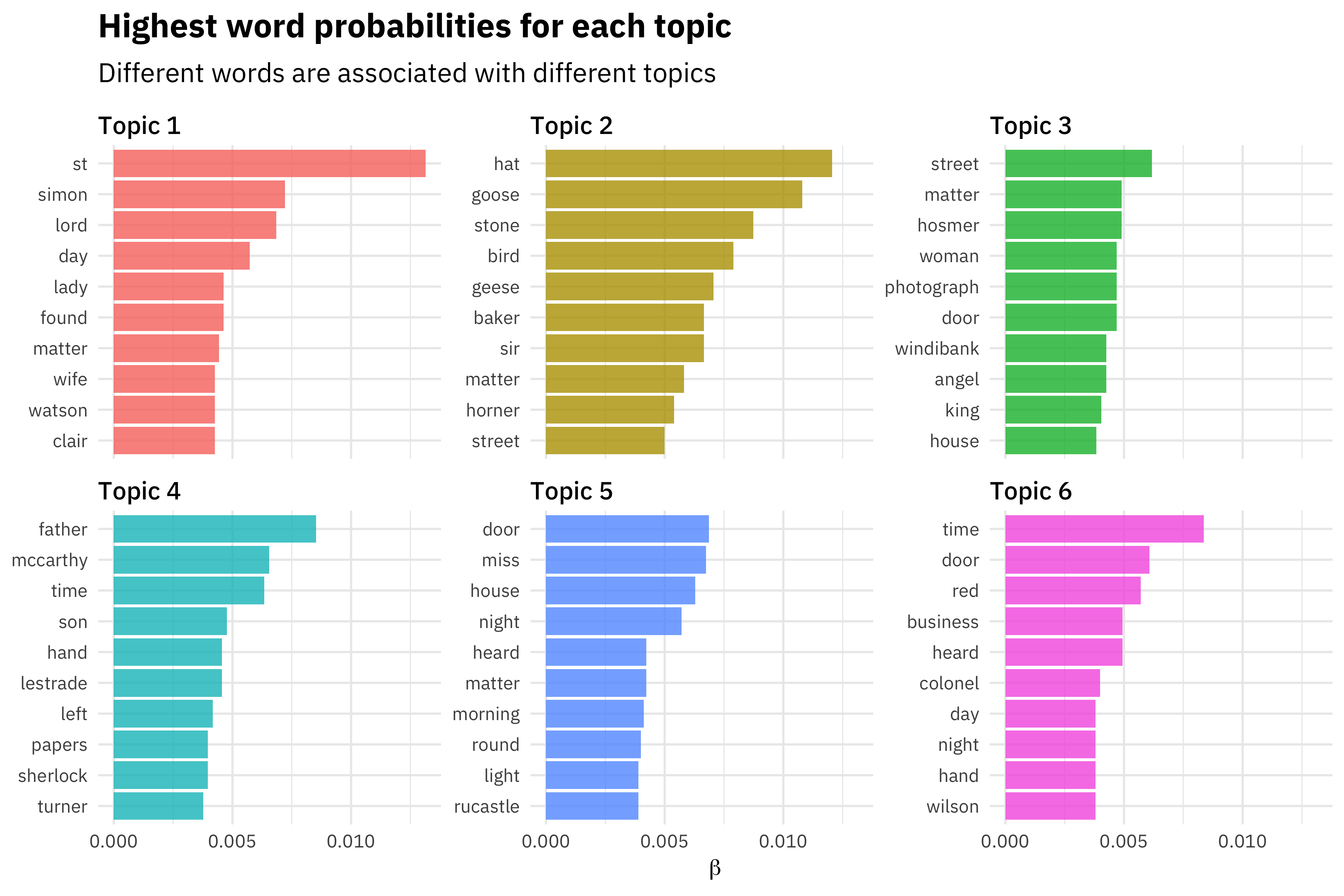
The tidied word-topic distributions can be used in standard ways for further analysis, such as a Silge plot of the highest probability words for each topic. But because the “words” in this simulation are just integers, and not semantically meaningful, we don’t construct such a plot here.

Finally, we compare fitted and true topic-document distributions. We extract topic-document distributions using the same tidy() function, specifying the matrix gamma and including the rotation above to align the fitted and true topics. Tile and parallel coordinates plots can be used to visualize all of the topic-document distributions. These show that the tmfast models successfully recover the overall association of each document’s journal with a distinctive topic.

Warning in tidy.tmfast(fitted, k, "gamma", rotation = rotation): Rotating
scores

However, the fitted topic-document distributions are flatter than the true ones. Consider the true and fitted distributions for document 1. Compared to the true distribution, the fitted distribution has a somewhat lower probability for topic V01 and a somewhat higher probability for the other topics.

This flatter distribution corresponds to greater entropy. In this simulation, the entropy of the fitted distributions are about 1 bit greater than those of the true distributions. This discrepancy tends to become worse with greater values of $k$.

Min. 1st Qu.  Median    Mean 3rd Qu.    Max.
 0.1006  0.6614  0.9715  1.0100  1.3311  2.5821

Min. 1st Qu.  Median    Mean 3rd Qu.    Max.
 0.8486  1.7040  1.9319  1.9129  2.1592  2.7673

To mitigate this problem, we add an optional renormalization step when converting document scores to topic-document distributions. Given a discrete probability distribution $P$ with components $p_{i}$ and entropy $H$, and a parameter $\beta$, we can define a new distribution $P^{\prime}$ with components

which has entropy

That is, we can choose a parameter $\beta$ that renormalizes $P$ to achieve a target entropy $H^{\prime}$. In LDA, the target entropy is the expected entropy for topic-document distributions drawn from the asymmetric Dirichlet prior. tmfast provides convenience functions for calculating this expected entropy; compare this to the mean entropy of the distributions in theta above. In actual applications, where the Dirichlet prior is an idealization, choosing $\alpha$ to set the target entropy is an important researcher degree of freedom. It is equivalent to choosing prior parameters in other topic modeling packages.

[1] 0.997604

Since solving the equation for $H^{\prime}$ for $\beta$ requires numerical optimization, it’s inefficient to do this every time we call tidy(), especially with large corpora. Instead, tmfast::target_power() is used to run this optimization once, and then return the mean value across all documents. We then use this single value of $\beta$ in all future calls to tidy().

[1] 1.539377

The renormalized topic-document distributions have closer entropy to $\theta$. The keep_original argument lets us compare the original and renormalized distributions.

Warning in tidy.tmfast(fitted, k, "gamma", rotation = rotation, exponent =
gamma_power, : Rotating scores

# A tibble: 1 x 2
  gamma gamma_rn
  <dbl>    <dbl>
1  1.91     1.03

We can now assess accuracy of the topic-document distributions. Above we used the hellinger() method for two matrices. The method for two dataframes requires specifying the id, topic, and probability columns. The tile plot shows that the true and fitted topics are aligned (because we used the rotation when extracting gamma_df above), and so again we can get an overall summary from the diagonal. Without renormalization, in the current simulation the mean Hellinger distance is 0.24 — not too bad, but perhaps larger than one would like. With larger values of $k$, this accuracy increases significantly. Renormalization keeps the mean distance around 0.13, comparable to the word-topic distributions.

Min. 1st Qu.  Median    Mean 3rd Qu.    Max.
0.08499 0.20131 0.23733 0.23770 0.27244 0.37585

Min. 1st Qu.  Median    Mean 3rd Qu.    Max.
0.04808 0.10195 0.12378 0.12518 0.14564 0.24868

STM has a slightly closer fit, with a mean Hellinger distance of 0.08.

Min. 1st Qu.  Median    Mean 3rd Qu.    Max.
0.03216 0.07148 0.08638 0.08823 0.10260 0.19884

We first retrieve all works in Project Gutenberg by our target authors: Jane Austen, Charlotte and Emily Brontë, Louisa May Alcott, George Eliot, Charles Dickens, HG Wells, and HP Lovecraft. For these authors, the memoise local cache ends up at about 286 MB.

We combine these results, and use tidytext::unnest_tokens() to convert the result into a long-format document-term matrix. Note that token extraction can take a long moment. We also construct a dataframe to link titles to authors in the topic model output.

# A tibble: 1,812,904 x 5
   gutenberg_id author                        title            term            n
          <int> <chr>                         <chr>            <chr>       <int>
 1           35 Wells, H. G. (Herbert George) The Time Machine _can_           1
 2           35 Wells, H. G. (Herbert George) The Time Machine _cancan_        1
 3           35 Wells, H. G. (Herbert George) The Time Machine _down_          1
 4           35 Wells, H. G. (Herbert George) The Time Machine _four_          1
 5           35 Wells, H. G. (Herbert George) The Time Machine _him_           1
 6           35 Wells, H. G. (Herbert George) The Time Machine _how_           1
 7           35 Wells, H. G. (Herbert George) The Time Machine _i_             1
 8           35 Wells, H. G. (Herbert George) The Time Machine _instantan˜     1
 9           35 Wells, H. G. (Herbert George) The Time Machine _minus_         1
10           35 Wells, H. G. (Herbert George) The Time Machine _nil_           1
# ... with 1,812,894 more rows

The number of works by each author varies widely, as does the total token count.

# A tibble: 10 x 2
   author                                 n
   <chr>                              <int>
 1 Alcott, Louisa May                    45
 2 Austen, Jane                          10
 3 Brontë, Anne                           2
 4 Brontë, Charlotte                      6
 5 Brontë, Emily                          1
 6 Dickens, Charles                      77
 7 Eliot, George                         18
 8 Lovecraft, H. P. (Howard Phillips)     7
 9 Shelley, Mary Wollstonecraft          17
10 Wells, H. G. (Herbert George)         70

[1] 253

‘summarise()‘ has grouped output by ’author’. You can override using the
‘.groups‘ argument.

# A tibble: 10 x 5
   author                                min  median    max   total
   <chr>                               <int>   <dbl>  <int>   <int>
 1 Dickens, Charles                     1364  31226  360502 6785632
 2 Wells, H. G. (Herbert George)        3958  64936. 470557 5224147
 3 Alcott, Louisa May                   2660  55483  194549 2977676
 4 Eliot, George                        1871 108236. 320413 2247001
 5 Austen, Jane                        23192 101879  784790 1652092
 6 Shelley, Mary Wollstonecraft        12514  53643  183856 1434844
 7 Brontë, Charlotte                    1416 138921  219783  699938
 8 Brontë, Anne                        68716 119946. 171177  239893
 9 Lovecraft, H. P. (Howard Phillips)   3654  12073   99008  160200
10 Brontë, Emily                      117082 117082  117082  117082

‘summarise()‘ has grouped output by ’author’. You can override using the
‘.groups‘ argument.

In line with a common rule of thumb in topic modeling, we aim for a vocabulary of about 10 times as many terms as documents in the corpus.

[1] 2530

tmfast provides two information-theoretic methods for vocabulary selection. Both are based on the idea of a two-player guessing game. I pick one of the documents from the corpus, then one of the terms from the document. I tell you the term, and you have to guess which document I picked. More informative terms have greater information gain (calculated as the Kullback-Leibler divergence) relative to a “baseline” distribution based purely on the process used to pick the document. The difference between the two methods is in the document-picking process. The ndH method assumes the document was picked uniformly at random from the corpus, so that no document is more likely to be picked than any other. The ndR method assumes document probability is proportional to the document length, so that shorter documents are less likely to be picked. This method implies that terms that are distinctive of shorter documents have high information gain, since they indicate “surprising” short documents.

On either method, the most informative terms are often typographical or OCR errors, since these only occur in a single document. To balance this, we multiply the information gain ($\Delta H$ for the uniform process, $\Delta R$ for the length-weighted process) by the log frequency of the term across the entire corpus ($\log n$). So ndH is shorthand for $\log(n)\Delta H$ while ndR is shorthand for $\log(n)\Delta R$.

17.518 sec elapsed

# A tibble: 116,449 x 5
   term           H    dH     n   ndH
   <chr>      <dbl> <dbl> <int> <dbl>
 1 kipps     0.125   7.86  1454  82.6
 2 dombey    0.386   7.60  1618  81.0
 3 boffin    0.108   7.87  1127  79.8
 4 pecksniff 0.366   7.62  1320  79.0
 5 gwendolen 0.239   7.74  1048  77.7
 6 lydgate   0.0235  7.96   867  77.7
 7 deronda   0.404   7.58  1155  77.1
 8 nicholas  0.977   7.01  1931  76.5
 9 tito      0.0835  7.90   811  76.3
10 squeers   0.253   7.73   895  75.8
# ... with 116,439 more rows

# A tibble: 116,449 x 5
   term           n    dR   ndR in_vocab
   <chr>      <int> <dbl> <dbl> <lgl>
 1 kipps       1454  7.48  78.6 TRUE
 2 hoopdriver   469  8.50  75.4 TRUE
 3 scrooge     1007  7.54  75.3 TRUE
 4 lewisham     575  8.03  73.6 TRUE
 5 benham       689  7.56  71.3 TRUE
 6 melville     243  8.97  71.1 TRUE
 7 bealby       458  8.04  71.0 TRUE
 8 veronica     659  7.52  70.4 TRUE
 9 bert         556  7.71  70.3 TRUE
10 christie    1797  6.43  69.5 TRUE
# ... with 116,439 more rows

The resulting term ranking of the two methods tend to be similar, but ndR is preferable in the current case because of the additional weight it gives to distinctive terms from shorter documents.

Warning: Using alpha for a discrete variable is not advised.

Warning: Using alpha for a discrete variable is not advised.

[1] "kipps"      "hoopdriver" "scrooge"    "lewisham"   "benham"
 [6] "melville"   "bealby"     "veronica"   "bert"       "christie"
[11] "sylvia"     "snitchey"   "boldheart"  "britling"   "castruccio"
[16] "bounderby"  "lillian"    "maggie"     "marjorie"   "craggs"
[21] "n’t"        "kemp"       "bab"        "redwood"    "harman"
[26] "cavor"      "chatteris"  "brumley"    "ammi"       "heathcliff"
[31] "tackleton"  "gladys"     "helwyze"    "tetterby"   "montgomery"
[36] "lodore"     "trafford"   "treherne"   "jill"       "ludovico"
[41] "tito"       "lomi"       "canaris"    "trotty"     "villiers"
[46] "falkner"    "doubledick" "amanda"     "gradgrind"  "linton"

‘summarise()‘ has grouped output by ’author’. You can override using the
‘.groups‘ argument.

0.801 sec elapsed

Without renormalization, most of the works are spread across a few topics, and the topics don’t clearly correspond to authors.

To renormalize, we need to choose a theoretical Dirichlet distribution.

[1] 0.997604

[1] 4.064884

After renormalization, there are distinctive topics for Alcott (4) and Wells (1 and 9). Austen, Anne Brontë, Emily Brontë, and some of Shelley’s works appear together in topic 3. Charlotte Brontë and some of Eliot’s and Shelley’s works split topic 5. Eliot and Lovecraft share topic 10. And Dickens’ works are spread across multiple topics, with 2, 6, and 8 appearing to be distinctive to him.

To aid interpretation, we create a crosswalk dataframe connecting topics to authors.

To explore these topics further, we turn to the word-topic distribution. These distributions could be renormalized, as with the topic-doc distributions. But the exponent for the word-topic distributions is usually quite close to 1, meaning renormalization doesn’t change these distributions very much.

[1] 8.597192

[1] 1.066448

We therefore skip renormalization and move directly to a Silge plot, showing the top 10 terms for each topic. tidytext::reorder_within() and tidytext::scale_x_reordered() are useful for constructing this plot.

# A tibble: 150 x 4
# Groups:   topic [10]
   token     topic    beta authors
   <chr>     <chr>   <dbl> <chr>
 1 empire    V01   0.0162  Wells
 2 britain   V01   0.0124  Wells
 3 peoples   V01   0.0122  Wells
 4 russia    V01   0.0117  Wells
 5 king      V01   0.0111  Wells
 6 asia      V01   0.0104  Wells
 7 socialism V01   0.00995 Wells
 8 section   V01   0.00971 Wells
 9 egypt     V01   0.00926 Wells
10 ii        V01   0.00892 Wells
# ... with 140 more rows

Most topics (2, 3, 4, 5, 6, 8, 9) focus on character names, with three of the four Dickens topics corresponding to The Pickwick Papers (topic 2), Oliver Twist (5), and David Copperfield (8). Wells’ topics appear to distinguish non-fiction essays (topic 1) from fiction (9). Topic 7 groups together Charlotte Brontë, Eliot, and Shelley based on the use of French. Topic 10 has a mix of character names with months of the year; it appears to be a “miscellaneous” topic, often created by topic models to accommodate documents that don’t fit elsewhere.

References

reBaglama, James, and Lothar Reichel. 2005. “Augmented Implicitly Restarted Lanczos Bidiagonalization Methods.” SIAM Journal on Scientific Computing 27 (1): 19–42. https://doi.org/10.1137/04060593X.
preBaglama, Jim, Lothar Reichel, and B. W. Lewis. 2022. “Irlba: Fast Truncated Singular Value Decomposition and Principal Components Analysis for Large Dense and Sparse Matrices.” https://cran.r-project.org/web/packages/irlba/index.html.
preBlei, David M., Andrew Y. Ng, and Michael I. Jordan. 2003. “Latent Dirichlet Allocation.” The Journal of Machine Learning Research 3: 993–1022. http://dl.acm.org/citation.cfm?id=944937.
preGelman, Andrew, and Eric Loken. 2013. “The Garden of Forking Paths: Why Multiple Comparisons Can Be a Problem, Even When There Is No ‘Fishing Expedition’ or ‘p-Hacking’ and the Research Hypothesis Was Posited Ahead of Time.” Downloaded January 30: 2014. http://www.stat.columbia.edu/˜gelman/research/unpublished/p_hacking.pdf.
preHicks, Daniel J. 2021. “Productivity and Interdisciplinary Impacts of Organized Research Units.” Quantitative Science Studies 2 (3): 990–1022. https://doi.org/10.1162/qss_a_00150.
preMalaterre, Christophe, and Francis Lareau. 2022. “The Early Days of Contemporary Philosophy of Science: Novel Insights from Machine Translation and Topic-Modeling of Non-Parallel Multilingual Corpora.” Synthese 200 (3): 242. https://doi.org/10.1007/s11229-022-03722-x.
preRoberts, Margaret E, Brandon M Stewart, and Dustin Tingley. 2019. “Stm: An R Package for Structural Topic Models.” Journal of Statistical Software 91 (October): 1–40. https://doi.org/10.18637/jss.v091.i02.
preRohe, Karl, and Muzhe Zeng. 2020. “Vintage Factor Analysis with Varimax Performs Statistical Inference.” arXiv. https://doi.org/10.48550/arXiv.2004.05387.
preSteegen, Sara, Francis Tuerlinckx, Andrew Gelman, and Wolf Vanpaemel. 2016. “Increasing Transparency Through a Multiverse Analysis.” Perspectives on Psychological Science 11 (5): 702–12. https://doi.org/10.1177/1745691616658637.