跳到论文正文
W Papers独立论文阅读器 arXiv:2305.01428 论文正文 计算阅读时间 · 0%
引用这篇论文根据当前论文元数据生成,正式投稿前建议核对。


Edge Universality of Random Regular Graphs of Growing Degrees

Horng-Tzer Yau
Abstract

We consider the statistics of extreme eigenvalues of random dd-regular graphs, with N𝔠⩽d⩽N1/3−𝔠N^{\mathfrak{c}}\leqslant d\leqslant N^{1/3-{\mathfrak{c}}} for arbitrarily small 𝔠>0{\mathfrak{c}}>0. We prove that in this regime, the fluctuations of extreme eigenvalues are given by the Tracy-Widom distribution. As a consequence, about 69% of dd-regular graphs have all nontrivial eigenvalues bounded in absolute value by 2​d−12\sqrt{d-1}.

University of Pennsylvania
E-mail: huangjy@wharton.upenn.edu

Harvard University
E-mail: htyau@math.harvard.edu

1 Introduction

Expander graphs are sparse graphs with strong connectivity property, and have numerous applications to the design of robust networks and the theory of error-correct coding [33]. The expansion property of a regular graph can be measured by its spectral gap. Ramanujan graphs are dd-regular graphs with the largest spectral gap, i.e. all nontrivial eigenvalues are bounded in absolute value by 2​d−12\sqrt{d-1}. They are the best possible expander graphs, at least as far as the spectral gap measure of expansion is concerned.

Ramanujan graphs were explicitly constructed when d=p+1d=p+1 with pp a prime power, by Lubotzky, Phillips and Sarnak [47] and independently by Margulis [50], using deep tools from number theory. More recently, in the breakthrough work [48, 49], Marcus, Spielman and Srivastava proved that there exist bipartite Ramanujan graphs of every degree. It still remains an interesting open problem whether there exist non-bipartite Ramanujan graphs of every degree. However, based on numerical simulation [52], it was observed a positive portion of random dd-regular graphs are Ramanujan.

We study the statistics of extreme eigenvalues of random dd-regular graphs, when the degree dd grows with the size of the graph. For random dd-regular graphs on NN vertices, it has been proven in [8] for N2/9+𝔠⩽d⩽N1/3−𝔠N^{2/9+{\mathfrak{c}}}\leqslant d\leqslant N^{1/3-{\mathfrak{c}}} and in [31] for N2/3+𝔠⩽d⩽N/2N^{2/3+{\mathfrak{c}}}\leqslant d\leqslant N/2, the fluctuations of extreme eigenvalues are given by the Tracy-Widom distribution from random matrix theory. In this work we generalize these edge universality results to the sparser regime N𝔠⩽d⩽N1/3−𝔠N^{\mathfrak{c}}\leqslant d\leqslant N^{1/3-{\mathfrak{c}}} for arbitrarily small 𝔠>0{\mathfrak{c}}>0. As a consequence, about 69% of dd-regular graphs on NN vertices with d3≪N⩽d1/𝔠d^{3}\ll N\leqslant d^{1/{\mathfrak{c}}} have all nontrivial eigenvalues bounded in absolute value by 2​d−12\sqrt{d-1}. This gives many Ramanujan graphs.

Universality for the edge statistics of Wigner matrices was first established by the moment method [57, 54, 39] under certain symmetry assumptions on the distribution of the matrix elements. The moment method was further developed in [53, 29] and [56]. A different approach to edge universality for Wigner matrices based on the direct comparison with corresponding Gaussian ensembles was developed in [58, 28, 22]. And later, a necessary and sufficient condition for edge universality of Wigner matrices were discovered in [46].

For the comparison argument, a key intermediate ingredient is the rigidity of extreme eigenvalues. For edge universality to be true, it is necessary that extreme eigenvalues fluctuate on scale O≺(N−2/3)\OO_{\prec}(N^{-2/3}). Main body of this paper is devoted to prove such optimal rigidity estimate. The proof is based on first constructing a higher order self-consistent equation for the Stieltjes transform of the empirical eigenvalue distribution, then computing high moments of the self-consistent equation by a recursive moment estimate, and proving it concentrates around zero. This approach was first introduced in [45] and further developed in [44, 35, 37, 32] to study sparse Erdős-Rényi graphs and in [8] to study sparse random dd-regular graphs.

For random dd-regular graphs, the self-consistent equation has a 1/d1/\sqrt{d} asymptotic expansion. The main challenge for the above approach is to show high moments of the self-consistent equation are close to zero, which requires cancellations of each order in the asymptotic expansion. [8] was able to explore the cancellation up to d−3/2d^{-3/2}, which implies the fluctuation of extreme eigenvalues is bounded by O≺(d−3+N−2/3)\OO_{\prec}(d^{-3}+N^{-2/3}). To get the optimal O≺(N−2/3)\OO_{\prec}(N^{-2/3}) fluctuation bound, we need to have cancellations up to d−𝔞/2d^{-{\mathfrak{a}}/2} for arbitrary large 𝔞⩾0{\mathfrak{a}}\geqslant 0. To achieve it, in this paper we combine the two steps, and construct the high order self-consistent equation and compute its high moments in one step. By construction, our high order self-consistent equation concentrates around zero. To identify the the self-consistent equation, we directly show the Stieltjes transform of the spectral measure of the infinite dd-regular tree satisfies the same equation. Thus extreme eigenvalues concentrate around the spectral edge of the infinite dd-regular tree, with optimal error O≺(N−2/3)\OO_{\prec}(N^{-2/3}).

The computation of the high order self-consistent equation boils down to estimate the following quantity (and its generalizations)

𝔼⁡[A𝒯​R​U],\displaystyle\mathbb{E}[A_{{\mathcal{T}}}RU], (1.1)

where 𝒯{\mathcal{T}} is a sub-tree graph (may not be connected), A𝒯A_{\mathcal{T}} is the indicator function that 𝒯{\mathcal{T}} is contained in the graph, RR is a polynomial of the Green’s function entries, and UU is any polynomial of the Stieltjes transform. To estimate (1.1), we resample each edge of the sub-tree 𝒯{\mathcal{T}}, and use it as a discrete integration by part. This generalizes the simple switching procedure, introduced in [11] to prove the local law of random dd-regular graphs.

For (1.1), there are three cases: i) If RR contains an off-diagonal Green’s function entry Gi​jG_{ij} such that i,ji,j are in different connected components of 𝒯{\mathcal{T}}, we show (1.1) is negligible. ii) If RR contains an off-diagonal Green’s function entry Gi​jG_{ij} such that i,ji,j are in the same connected component of 𝒯{\mathcal{T}}, we show (1.1) is a finite linear combination of terms in the same form, but with some extra factors of 1/d1/\sqrt{d}. iii) If RR contains only diagonal Green’s function entries, the leading term is obtained by replacing RR by a power of the Stieltjes transform of the empirical measure, and the higher order terms are again in the form of (1.1) with some extra factors of 1/d1/\sqrt{d}. By repeating this procedure, we eventually obtain a polynomial of the Stieltjes transform of the empirical measure, which leads to the self-consistent equation.

To prove the convergence to the Tracy-Widom distribution, we took a dynamical approach, which was original developed to prove the bulk universality of Wigner matrices [24, 25, 19, 41, 42, 17, 21, 26]. We interpolate the adjacency matrix with the Gaussian orthogonal ensemble (GOE). The eigenvalues at each time slice have the same law as Dyson Brownian motion (DBM). For sufficiently regular initial data, it has been proven in [43], after short time the eigenvalue statistics at the spectral edge of DBM agree with GOE. With the optimal edge rigidity as input, [43] implies the edge universality holds for adjacency matrix plus a small Gaussian component. Our main contribution is to show the edge statistics do not change along the interpolation, thus edge universality holds for the original adjacency matrix. The main challenge is to keep track the edge location LtL_{t} along the interpolation. At each time tt, we can construct a high order self-consistent equation, which governs the spectral of the interpolated matrix. We discover that the time derivative of LtL_{t} is given by the spatial derivative of the corresponding high order self-consistent equation with a negligible error. This allows us to build a dynamical framework around LtL_{t} and show the edge statistics do not change.

It is worth to compare edge results of sparse Erdős–Rényi graphs and random dd-regular graphs. Thanks to a series of papers [32, 22, 45, 44, 35, 37], the edge statistics of Erdős–Rényi graphs G⁡(N,p)G(N,p) with N​p⩾N𝔠Np\geqslant N^{\mathfrak{c}} are now well understood. When the average degree p​N≫N1/3pN\gg N^{1/3}, extreme eigenvalues have Tracy-Widom fluctuations [22, 45]. However, when N𝔠⩽p​N≪N1/3N^{{\mathfrak{c}}}\leqslant pN\ll N^{1/3} the extreme eigenvalues have Gaussian fluctuations, given by the fluctuation of the total number of edges [35, 32]. The higher order fluctuations are given by a sum of an infinite hierarchy of subgraph counting random variables which are asymptotically joint Gaussian [44]. Surprisingly, up to this explicit random shift, the fluctuations of extreme eigenvalues are still given by the Tracy-Widom distribution [37]. For random dd-regular graphs, the fluctuations of those subgraph counting quantities are negligible. Extreme eigenvalues concentrate around a deterministic spectral edge and converge to the Tracy-Widom distribution. In the same regime, bulk universality for Erdős–Rényi graphs and random dd-regular graphs are also known [7, 34, 22].

For Erdős–Rényi graphs in the sparser regime N​p=O⁡(ln⁡N)Np=\OO(\ln N), there exists a critical value b∗=1/(ln⁡4−1)b_{*}=1/(\ln 4-1) such that if N​p⩾b∗​ln⁡N/NNp\geqslant b_{*}\ln N/N, the extreme eigenvalues of the normalized adjacency matrix converge to ±2\pm 2 [13, 4, 59, 14] and all the eigenvectors are delocalized [5, 23]. For (ln⁡ln⁡N)4≪N​p<b∗​ln⁡N/N(\ln\ln N)^{4}\ll Np<b_{*}\ln N/N, there are outlier eigenvalues [59, 4]. The spectrum splits into three phases: a delocalized phase in the bulk, a fully localized phase near the spectral edge, and a semilocalized phase in between [6, 3]. Moreover, the joint fluctuations of the eigenvalues near the spectral edges form a Poisson point process. For random dd-regular graphs with any fixed degree d⩾3d\geqslant 3, all the eigenvectors are delocalized [9, 36]. The fluctuation of extreme eigenvalues is still conjectured to be the Tracy-Widom distribution [52]. This conjecture is still quite open, but we do know the extreme eigenvalues concentrate around ±2​d−1\pm 2\sqrt{d-1} with an error O⁡((ln⁡ln⁡N/ln⁡N)2)\OO((\ln\ln N/\ln N)^{2}) [16, 30], which recently was improved by the two authors to a polynomial bound O⁡(N−𝔠)\OO(N^{-{\mathfrak{c}}}) [36].

Organization. We define the model and present the main results in the rest of Section 1. In Section 2, we recall the local law for random dd-regular graphs from [12], and state our improved estimates for the Stieltjes transform of the empirical eigenvalue distribution. In Section 3, we discuss simple switchings, and use them as a discrete integration by part. In Section 4, we collect some estimates and notations on Green’s function. In Section 5, we construct the high order self-consistent equation, and show its moments are close to zero. In Section 6, we identify the self-consistent equation and prove the optimal edge rigidity. In Section 7, we prove the edge universality result by interpolating with GOE.

Notations. We use CC to represent large universal constants, and cc small universal constants, which may be different from line by line. Let Y⩾0Y\geqslant 0. We write X≲YX\lesssim Y or Y≳XY\gtrsim X if there exists a constant C>0C>0, such that X⩽C​YX\leqslant CY. We write X≍YX\asymp Y if there exists a constant C>0C>0 such that Y/C⩽X⩽Y/CY/C\leqslant X\leqslant Y/C. We use ℂ+{\mathbb{C}}_{+} to represent the upper half plane. For any index set 𝒎={m1,m2,⋯,mr}\bm{m}=\{m_{1},m_{2},\cdots,m_{r}\}, we write

∑∗𝒎=∑1⩽m1,m2,⋯,mr⩽N,distinct.\displaystyle\sum^{*}_{\bm{m}}=\sum_{1\leqslant m_{1},m_{2},\cdots,m_{r}\leqslant N,\atop\text{distinct}}. (1.2)

Acknowledgements The research of J.H. is supported by NSF grant DMS-2054835. The research of H-T.Y. is supported by NSF grants DMS-1855509, DMS-2153335 and a Simons Investigator award. J.H. wants to thank Yukun He for carefully reading the manuscript of the paper, and pointing some mistakes.

1.1 Main results

Let ℙ\mathbb{P} be the uniform probability measure on the set of dd-regular graphs on NN vertices. We identify a graph with its adjacency matrix A=(Ai​j)∈{0,1}N×NA=(A_{ij})\in\{0,1\}^{N\times N}, defined as Ai​j=1A_{ij}=1 if and only if ii and jj are adjacent. Thus, ℙ\mathbb{P} is the uniform probability measure on the set of symmetric matrices A∈{0,1}N×NA\in\{0,1\}^{N\times N} satisfying ∑j=1NAi​j=d\sum_{j=1}^{N}A_{ij}=d and Ai​i=0A_{ii}=0 for all i=1,…,Ni=1,\dots,N.

Since AA is dd-regular, it is immediate that AA has a trivial eigenvalue dd with associated eigenvector (1,1,…,1)∗(1,1,\dots,1)^{*}. Moreover, by the Perron-Frobenius theorem, all other eigenvalues are bounded in absolute value by dd. For convenience, we shall consider the normalized adjacency matrix

H:=A/d−1.H\mathrel{\mathop{:}}=A/\sqrt{d-1}. (1.3)

We denote its eigenvalues by λ1=d/d−1⩾λ2⩾⋯⩾λN⩾−d/d−1\lambda_{1}=d/\sqrt{d-1}\geqslant\lambda_{2}\geqslant\cdots\geqslant\lambda_{N}\geqslant-d/\sqrt{d-1}, and corresponding orthonormal eigenvectors 𝒖1,𝒖2,⋯,𝒖N{\bm{u}}_{1},{\bm{u}}_{2},\cdots,{\bm{u}}_{N}.

Our main result is about the limiting distribution of the extremal eigenvalues. For 1≪d≪N1/31\ll d\ll N^{1/3}, extreme eigenvalues of random dd-regular graphs converge to the Tracy-Widom distribution.

Theorem 1.1.

Fix arbitrarily small 𝔠>0{\mathfrak{c}}>0, and an integer k⩾1k\geqslant 1, let F:ℝk→ℝF:\mathbb{R}^{k}\to\mathbb{R} be a bounded test function with bounded derivatives. For N𝔠⩽d⩽N1/3−𝔠N^{{\mathfrak{c}}}\leqslant d\leqslant N^{1/3-{\mathfrak{c}}}, there is a universal constant 𝔢>0{\mathfrak{e}}>0 so that,

𝔼H[F(N2/3(λ2−2),⋯,N2/3(λk+1−2)]=𝔼G​O​E​[F⁡(N2/3​(μ1−2),⋯,N2/3​(μk−2))]+𝒪⁡(N−𝔢),\displaystyle\begin{split}&\phantom{{}={}}\mathbb{E}_{H}[F(N^{2/3}(\lambda_{2}-2),\cdots,N^{2/3}(\lambda_{k+1}-2)]\\ &=\mathbb{E}_{GOE}[F(N^{2/3}(\mu_{1}-2),\cdots,N^{2/3}(\mu_{k}-2))]+\mathcal{O}\left(N^{-{\mathfrak{e}}}\right),\end{split} (1.4)

provided NN is large enough. The second expectation is with respect to a GOE matrix with eigenvalues μ1⩾μ2⩾⋯⩾μN\mu_{1}\geqslant\mu_{2}\geqslant\cdots\geqslant\mu_{N}. Analogous results hold for the smallest eigenvalues.

Since the seminal works [47, 50], it remains an open problem if there exist infinite families of Ramanujan graphs with any degree dd. For the bipartite case, an affirmative answer was given in the recent breakthrough work [48, 49]; and see [20] for polynomial time algorithm of this construction. The problem for non-bipartite case is still open. And it is conjectured in [55, 52], a positive fraction of regular graphs of fixed dd is Ramanujan. As emphasized in [55], the Tracy–Widom1 distribution has about 83%83\% of its mass on the set {x:x<0}\{x:x<0\}. Therefore Theorem 1.1 implies 83%83\% of dd-regular graphs have the second eigenvalue less than 2​d−12\sqrt{d-1}, provided that NN and dd obey the conditions of Theorem 1.1. The proof of Theorem 1.1 can be extended to show that in the regime N𝔠⩽d⩽N1/3−𝔠N^{{\mathfrak{c}}}\leqslant d\leqslant N^{1/3-{\mathfrak{c}}} the largest and smallest nontrivial eigenvalues converge in distribution to independent Tracy–Widom1 distributions; see Remarks 7.7 and 7.9 below. As a consequence, we have the following result.

Corollary 1.2.

For dd large enough and d3≪N⩽d1/𝔠d^{3}\ll N\leqslant d^{1/{\mathfrak{c}}}, about 69%69\%11 1 In [8], the percentage is 27%27\%, which is a mistake. This percentage 27%27\% is computed as 52%×52%52\%\times 52\%, using that the Tracy–Widom1 distribution has about 52%52\% of its mass on the set {x:x<0}\{x:x<0\}. The number 52%52\% is wrong, and should be 83%83\%. of dd-regular graphs on NN vertices have all nontrivial eigenvalues bounded in absolute value by 2​d−12\sqrt{d-1}.

Although Corollary 1.2 does not give infinite families of Ramanujan graphs, it does give a lot Ramanujan graphs.

Unless stated otherwise, all quantities in this paper depend on the fundamental parameter NN, and we omit this dependence from our notation. For the following statements, for deterministic NN-dependent quantities XX and YY we write X≪YX\ll Y if X⩽N−ε​YX\leqslant N^{-\varepsilon}Y for some fixed ε>0\varepsilon>0 and N⩾N⁡(ε)N\geqslant N(\varepsilon) large enough. For NN-dependent random (or deterministic) variables XX and YY, we say YY stochastically dominates XX, if for any ε>0\varepsilon>0 and D>0D>0, then

ℙ⁡(X⩽Nε​Y)⩾1−N−D,\mathbb{P}(X\leqslant N^{\varepsilon}Y)\geqslant 1-N^{-D},

for N⩾N⁡(ε,D)N\geqslant N(\varepsilon,D) large enough, and we write X≺YX\prec Y or X=𝒪≺​(Y)X=\mathcal{O}_{\prec}(Y). We say an event Ω\Omega holds with overwhelming probability, if for any D>0D>0, ℙ⁡(Ω)⩾1−N−D\mathbb{P}(\Omega)\geqslant 1-N^{-D} for N⩾N⁡(D)N\geqslant N(D) large enough.

2 Eigenvalue Rigidity Estimates

We consider the adjacency matrix AA restricted to the subspace orthogonal to the vector 𝟏:=(1,…,1)∗{\bf 1}\mathrel{\mathop{:}}=(1,\dots,1)^{*}. More precisely, let P⟂:ℝN→ℝNP_{\perp}\vcentcolon{\mathbb{R}}^{N}\to{\mathbb{R}}^{N} be the orthogonal projection onto 𝟏⟂{\bf 1}^{\perp}, explicitly given by P⟂=I−𝟏𝟏∗/NP_{\perp}=I-{\bf 1}{\bf 1^{*}}/N where II is the N×NN\times N identity matrix. Since HH is the normalized adjacency matrix of a regular graph, the matrices HH and P⟂P_{\perp} commute: H​P⟂=P⟂​HHP_{\perp}=P_{\perp}H.

For a spectral parameter z∈ℂ+:={z∈ℂ:Im[z]>0}z\in{\mathbb{C}}_{+}\mathrel{\mathop{:}}=\{z\in{\mathbb{C}}\vcentcolon\mathop{\mathrm{Im}}[z]>0\} we define the Green’s function by

G⁡(z):=P⟂​(H−z)−1​P⟂=∑i=2N𝒖i​𝒖i∗λi−z,G(z)\mathrel{\mathop{:}}=P_{\perp}(H-z)^{-1}P_{\perp}=\sum_{i=2}^{N}\frac{{\bm{u}}_{i}{\bm{u}}_{i}^{*}}{\lambda_{i}-z},

we remark that the projection P⟂P_{\perp} kills the largest eigenvalue. Thus, GG and (H−z)−1(H-z)^{-1} agree on the image of P⟂P_{\perp}, which is the subspace of ℝN{\mathbb{R}}^{N} perpendicular to 𝟏\bm{1}. The Green’s function satisfies the relation

G⁡(z)​H=H​G​(z)=z​G​(z)+P⟂=z​G​(z)+(I−𝟏𝟏∗/N).\displaystyle G(z)H=HG(z)=zG(z)+P_{\perp}=zG(z)+(I-{\bf 1}{\bf 1^{*}}/N). (2.1)

Moreover,

∑i=1NGi​j​(z)=∑j=1NGi​j​(z)=0.\sum_{i=1}^{N}G_{ij}(z)=\sum_{j=1}^{N}G_{ij}(z)=0. (2.2)

We denote the normalized trace of GG, which is also the Stieltjes transform of the empirical spectral measure of H|𝟏⟂H|_{\bm{1}^{\perp}}, by

m⁡(z):=1N​∑iGi​i​(z)=∑i=2N1λi−z.m(z)\mathrel{\mathop{:}}=\frac{1}{N}\sum_{i}G_{ii}(z)=\sum_{i=2}^{N}\frac{1}{\lambda_{i}-z}. (2.3)

We refer to m⁡(z)m(z) simply as the Stieltjes transform. Our goal is to approximate m⁡(z)m(z) by md​(z)m_{d}(z), the Stieltjes transform of the Kesten–McKay law [38],

md(z):=∫ℝρd​(x)x−zdx,ρd(x):=(1+1d−1−x2d)−1[4−x2]+2​π.\displaystyle m_{d}(z)\mathrel{\mathop{:}}=\int_{\mathbb{R}}\frac{\rho_{d}(x)}{x-z}{\rm d}x,\qquad\rho_{d}(x)\mathrel{\mathop{:}}=\left(1+\frac{1}{d-1}-\frac{x^{2}}{d}\right)^{-1}\frac{\sqrt{[4-x^{2}]_{+}}}{2\pi}.

The Kesten–McKay law ρd\rho_{d} is the spectral measure at any vertex of the infinite dd-regular tree (see, for example, [2] or [10, Section 5]). It has support [−2,2][-2,2] in our normalization. The Stieltjes transform md​(z)m_{d}(z) is explicitly given by

md​(z)=−(z+dd−1​msc​(z))−1,m_{d}(z)=-\left({z+\frac{d}{d-1}m_{\rm sc}(z)}\right)^{-1}, (2.4)

where msc​(z)m_{\rm sc}(z) is the Stieltjes transform of the Wigner semicircle law,

msc(z):=∫ℝρsc​(x)x−zdx,ρsc(x):=[4−x2]+2​π,m_{\rm sc}(z)\mathrel{\mathop{:}}=\int_{\mathbb{R}}\frac{\rho_{\text{sc}}(x)}{x-z}{\rm d}x,\qquad\rho_{\text{sc}}(x)\mathrel{\mathop{:}}=\frac{\sqrt{[4-x^{2}]_{+}}}{2\pi}, (2.5)

satisfying the self-consistent equation

1+z​msc​(z)+msc2​(z)=0.1+zm_{\rm sc}(z)+m_{\rm sc}^{2}(z)=0. (2.6)

Later we shall use that, alternatively, md​(z)m_{d}(z) can be characterized by the self-consistent equation, which follows from rearranging (2.4)

P∞​(z,md​(z))=0,P∞​(z,w)=1+z​w+dd−1​w2+∑k⩾2(−2)k−1​(2​k−3)!!k!​d(d−1)k​w2​k.\displaystyle P_{\infty}(z,m_{d}(z))=0,\quad P_{\infty}(z,w)=1+zw+\frac{d}{d-1}w^{2}+\sum_{k\geqslant 2}\frac{(-2)^{k-1}(2k-3)!!}{k!}\,\frac{d}{(d-1)^{k}}\,w^{2k}. (2.7)

We fix a large constant 𝔎>0{\mathfrak{K}}>0 and define the spectral domain

𝐃:={z=E+iη:−𝔎⩽E⩽𝔎,0<η⩽𝔎,Nηmin⁡{|E−2|,|E+2|}+η⩾N1/𝔎}.\mathbf{D}\mathrel{\mathop{:}}=\{z=E+\mathrm{i}\eta\vcentcolon-{\mathfrak{K}}\leqslant E\leqslant{\mathfrak{K}},0<\eta\leqslant{\mathfrak{K}},N\eta\sqrt{\min\{|E-2|,|E+2|\}+\eta}\geqslant N^{1/{\mathfrak{K}}}\}. (2.8)

Here, and throughout the following, we use the notation z=E+i​ηz=E+\mathrm{i}\eta for the real and imaginary parts of zz. The local semicircle law for random regular graphs [12] shows that m⁡(z)m(z) is approximated by md​(z)m_{d}(z) to order 1/d1/\sqrt{d} (up to logarithmic corrections), at least away from the edges ±2\pm 2 of the spectral measure. The next result follows from [12, Theorem 1.1]. We remark that [12, Theorem 1.1] gives a better estimate for Λd\Lambda_{\rm d} for zz away from the edge ±2\pm 2, but the following weaker form is enough for our purpose.

Theorem 2.1 ([12, Theorem 1.1]).

Let z=E+i​η∈ℂ+z=E+\mathrm{i}\eta\in{\mathbb{C}}_{+}, define the deterministic control parameters

Λo(z):=1N​η+1d+d3/2N,Λd(z):=(1N​η+1d+d3/2N)1/2.\Lambda_{\rm o}(z)\mathrel{\mathop{:}}=\frac{1}{\sqrt{N\eta}}+\frac{1}{\sqrt{d}}+\frac{d^{3/2}}{N},\quad\Lambda_{\rm d}(z)\mathrel{\mathop{:}}=\left(\frac{1}{\sqrt{N\eta}}+\frac{1}{\sqrt{d}}+\frac{d^{3/2}}{N}\right)^{1/2}. (2.9)

Fix small 𝔠>0{\mathfrak{c}}>0, we have, for N𝔠⩽d⩽N2/3−𝔠N^{\mathfrak{c}}\leqslant d\leqslant N^{2/3-{\mathfrak{c}}} and all z∈𝐃z\in\mathbf{D} from (2.8)

maxi≠j⁡|Gi​j​(z)|≺Λo​(z),maxi⁡|Gi​i​(z)−msc​(z)|≺Λd​(z).\displaystyle\max_{i\neq j}|G_{ij}(z)|\prec\Lambda_{\rm o}(z),\quad\max_{i}|G_{ii}(z)-m_{\rm sc}(z)|\prec\Lambda_{\rm d}(z). (2.10)

Averaging over the index ii, the estimate (2.10) implies an estimate on the Stieltjes transform m⁡(z)m(z). Using additional cancelations from this average, in this paper we shall derive a more precise estimate from which we obtain our results about the extremal eigenvalues.

Theorem 2.2.

For N𝔠⩽d⩽N1/3−𝔠N^{\mathfrak{c}}\leqslant d\leqslant N^{1/3-{\mathfrak{c}}}, uniform for z=E+i​η∈𝐃z=E+\mathrm{i}\eta\in\mathbf{D}, the Stieltjes transform of random dd-regular graphs satisfies

|m⁡(z)−md​(z)|≺{1N​η+dN​dist⁡(z,±2),−2⩽E⩽2,1dist⁡(z,±2)​(1N​η1/2+1(N​η)2+dN),|E|⩾2.\displaystyle|m(z)-m_{d}(z)|\prec\left\{\begin{array}[]{cc}\frac{1}{N\eta}+\frac{d}{N\sqrt{\dist(z,\pm 2)}},&-2\leqslant E\leqslant 2,\\ \frac{1}{\sqrt{\dist(z,\pm 2)}}\left(\frac{1}{N\eta^{1/2}}+\frac{1}{(N\eta)^{2}}+\frac{d}{N}\right),&|E|\geqslant 2.\end{array}\right.

We denote the classical eigenvalue locations of the Kesten-McKay distribution ρd\rho_{d} as γ2>γ3>⋯>γN\gamma_{2}>\gamma_{3}>\cdots>\gamma_{N},

k−1/2N−1=∫γk2ρd​(x)​𝑑x,2⩽k⩽N.\displaystyle\frac{k-1/2}{N-1}=\int_{\gamma_{k}}^{2}\rho_{d}(x){\rm d}x,\quad 2\leqslant k\leqslant N.

Then we have the following rigidity estimates

|λk−γk|≺dN+1N2/3​min⁡{k−1,N+1−k}1/3,2⩽k⩽N.\displaystyle|\lambda_{k}-\gamma_{k}|\prec\frac{d}{N}+\frac{1}{N^{2/3}\min\{k-1,N+1-k\}^{1/3}},\quad 2\leqslant k\leqslant N. (2.13)
Remark 2.3.

We remark the rigidity estimates (2.13) is not sharp for bulk eigenvalues because of the extra term d/Nd/N. However, since d/N≪1/N2/3d/N\ll 1/N^{2/3}, the estimate is sharp for extreme eigenvalues.

3 Simple Switchings

Our analysis makes use of switchings for regular graphs and also makes some use of the invariance under the permutation of vertices. We use ideas related to those introduced in [12, 7], to which we also refer for references to other uses of switchings.

3.1 Switchings

As in [12, 7], we define the signed adjacency matrices

(Δi​j)a​b:=δi​aδj​b+δi​bδj​a,ξi​jk​ℓ:=Δi​j+Δk​ℓ−Δi​k−Δj​ℓ,(\Delta_{ij})_{ab}\mathrel{\mathop{:}}=\delta_{ia}\delta_{jb}+\delta_{ib}\delta_{ja},\qquad\xi_{ij}^{k\ell}\mathrel{\mathop{:}}=\Delta_{ij}+\Delta_{k\ell}-\Delta_{ik}-\Delta_{j\ell}, (3.1)

corresponding to a switching of the edges i​jij and k​ℓk\ell; see Figure 1. For any indices i,j,k,ℓi,j,k,\ell, we denote the indicator function that the edges i​jij and k​ℓk\ell are switchable (i.e. the edges i​jij and k​ℓk\ell are present and the switching again results in a simple regular graph) by

χi​jk​ℓ​(A)=Ai​j​Ak​ℓ​(1−Ai​k)​(1−Aj​l).\displaystyle\chi_{ij}^{k\ell}(A)=A_{ij}A_{k\ell}(1-A_{ik})(1-A_{jl}). (3.2)
Refer to caption
Figure 1: Left Panel: A simple switching is given by replacing the solid edges by the dashed edges. Right Panel: An example of forest 𝒯{\mathcal{T}}, which consists of three connected components, i.e. θ⁡(𝒯)=3\theta({\mathcal{T}})=3.

The following concept of forest will be used throughout the paper.

Definition 3.1.

(Forest). By a forest we mean a finite simple graph which is a union of trees: 𝒯=(𝐢⁡(𝒯),E⁡(𝒯))=(𝐢,E){\mathcal{T}}=({\bf i}({\mathcal{T}}),E({\mathcal{T}}))=({\bf i},E). Here 𝐢∈[[N]]{\bf i}\in[\![{N}]\!] is a finite set of distinct vertices, EE is a finite set of edges, and each edge e∈Ee\in E connects {ie,ie′}∈𝐢\{i_{e},i^{\prime}_{e}\}\in{\bf i}. We denote the number of connected components of 𝒯{\mathcal{T}} as θ⁡(𝒯)\theta({\mathcal{T}}). We remark that 𝒯{\mathcal{T}} may contain singletons. See Figure 1 for an example.

Given a forest 𝒯=(𝐢,E){\mathcal{T}}=({\bf i},E), we denote

A𝒯=∏e∈EAie​ie′,\displaystyle A_{{\mathcal{T}}}=\prod_{e\in E}A_{i_{e}i^{\prime}_{e}},

If 𝒯{\mathcal{T}} consists of only singletons, i.e. E=∅E=\emptyset, then we simply define A𝒯=1A_{{\mathcal{T}}}=1. In the rest of this section, we use switchings to estimate terms in the following forms

𝔼⁡[A𝒯​F​(A)],𝔼⁡[A𝒯​Ai​k​F​(A)],𝔼⁡[A𝒯​Aj​k​F​(A)],i∈𝐢,j,k∉𝐢\displaystyle\mathbb{E}\left[A_{{\mathcal{T}}}F(A)\right],\quad\mathbb{E}\left[A_{{\mathcal{T}}}A_{ik}F(A)\right],\quad\mathbb{E}\left[A_{{\mathcal{T}}}A_{jk}F(A)\right],\quad i\in{\bf i},j,k\not\in{\bf i}

where FF is any function depending on the random graph AA. (Later, we shall take FF to be a polynomial of the Green’s function entries {Gi​j}i,j∈[[N]]\{G_{ij}\}_{i,j\in[\![{N}]\!]} and the Stieltjes transform mm.)

Proposition 3.2.

Given a forest 𝒯=(𝐢,E){\mathcal{T}}=({\bf i},E), and a function FF which depends on the random graph AA. For each edge e∈Ee\in E, we associate another edge {je,je′}∈[[N]]\{j_{e},j^{\prime}_{e}\}\in[\![{N}]\!], and denote 𝐣={je,je′}e∈E{\bf j}=\{j_{e},j^{\prime}_{e}\}_{e\in E}. If the indices 𝐢,𝐣\bf i,\bf j are distinct, we have the identity

𝔼⁡[F⁡(A)​∏e∈Eχie​ie′je​je′​(A)]=𝔼⁡[F⁡(A+∑e∈Eξie​ie′je​je′)​∏e∈Eχie​jeie′​je′​(A)].\displaystyle\mathbb{E}\left[F(A)\prod_{e\in E}\chi_{i_{e}i^{\prime}_{e}}^{j_{e}j^{\prime}_{e}}(A)\right]=\mathbb{E}\left[F\left(A+\sum_{e\in E}\xi_{i_{e}i^{\prime}_{e}}^{j_{e}j^{\prime}_{e}}\right)\prod_{e\in E}\chi_{i_{e}j_{e}}^{i^{\prime}_{e}j^{\prime}_{e}}(A)\right]. (3.3)

If the index i∈𝐢i\in{\bf i} and the indices 𝐢​j​k​m​ℓ{\bf i}jkm\ell are distinct, we have the identities

𝔼⁡[A𝒯​χi​km​ℓ​(A)​F​(A)]=𝔼⁡[A𝒯​χi​mk​ℓ​(A)​F​(A+ξi​km​ℓ)],𝔼⁡[A𝒯​χj​km​ℓ​(A)​F​(A)]=𝔼⁡[A𝒯​χj​mk​ℓ​(A)​F​(A+ξj​km​ℓ)],\displaystyle\begin{split}&\mathbb{E}\left[A_{{\mathcal{T}}}\chi_{ik}^{m\ell}(A)F(A)\right]=\mathbb{E}\left[A_{{\mathcal{T}}}\chi_{im}^{k\ell}(A)F(A+\xi_{ik}^{m\ell})\right],\\ &\mathbb{E}\left[A_{{\mathcal{T}}}\chi_{jk}^{m\ell}(A)F(A)\right]=\mathbb{E}\left[A_{{\mathcal{T}}}\chi_{jm}^{k\ell}(A)F(A+\xi_{jk}^{m\ell})\right],\end{split} (3.4)

where the indicator function χ\chi is as defined in (3.2).

Proof.

Define the sets of graphs

𝒢1={A:∏e∈Eχie​ie′je​je′(A)=1},𝒢2={A:∏e∈Eχie​jeie′​je′(A)=1}.\displaystyle\begin{split}{\mathcal{G}}_{1}=\left\{A:\prod_{e\in E}\chi_{i_{e}i^{\prime}_{e}}^{j_{e}j^{\prime}_{e}}(A)=1\right\},\quad{\mathcal{G}}_{2}=\left\{A:\prod_{e\in E}\chi_{i_{e}j_{e}}^{i^{\prime}_{e}j^{\prime}_{e}}(A)=1\right\}.\end{split}

By our assumption that the indices 𝐢,𝐣{\bf i},{\bf j} are distinct, there is a simple bijection between 𝒢1{\mathcal{G}}_{1} and 𝒢2{\mathcal{G}}_{2}, namely

A∈𝒢2↦A+∑e∈Eξie​ie′je​je′∈𝒢1.\displaystyle A\in{\mathcal{G}}_{2}\mapsto A+\sum_{e\in E}\xi_{i_{e}i^{\prime}_{e}}^{j_{e}j^{\prime}_{e}}\in{\mathcal{G}}_{1}. (3.5)

Since ℙ\mathbb{P} is the uniform probability measure on dd-regular graphs, the claim follows from (3.5).

The two identities in (3.4) can be proven in the same way, we will only give the proof of the first one. We define the sets of graphs 𝒢1={A:A𝒯​χi​km​ℓ​(A)=1}{\mathcal{G}}_{1}=\left\{A:A_{{\mathcal{T}}}\chi_{ik}^{m\ell}(A)=1\right\} and 𝒢2={A:A𝒯​χi​mk​ℓ​(A)=1}.{\mathcal{G}}_{2}=\left\{A:A_{{\mathcal{T}}}\chi_{im}^{k\ell}(A)=1\right\}. By our assumption that the indices 𝐢​k​m​ℓ{\bf i}km\ell are distinct, there is a simple bijection between 𝒢1{\mathcal{G}}_{1} and 𝒢2{\mathcal{G}}_{2}: A∈𝒢2↦A+ξi​km​ℓ∈𝒢1,A\in{\mathcal{G}}_{2}\mapsto A+\xi_{ik}^{m\ell}\in{\mathcal{G}}_{1}, and the claim follows.

∎

3.2 Discrete Integration by Part

We define the discrete derivative operators induced by the simple switchings, which will be used in the rest of this paper.

Definition 3.3.

For any symmetric matrix ξ=∑a=1bξia​jaka​ℓa\xi=\sum_{a=1}^{b}\xi_{i_{a}j_{a}}^{k_{a}\ell_{a}} (recall from (3.1)) for some fixed b∈ℕb\in\mathbb{N}, we denote the vertex set 𝐕(ξ)=∪a=1b{ia,ja,ka,ℓa}\bm{V}(\xi)=\cup_{a=1}^{b}\{i_{a},j_{a},k_{a},\ell_{a}\} and define the discrete and continuous derivative operator as

DξF(A):=F(A+ξ)−F(A),∂ξF(A):=d−1∂tF(A+tξ)|t=0.D_{\xi}F(A)\mathrel{\mathop{:}}=F(A+\xi)-F(A),\quad\partial_{\xi}F(A)\mathrel{\mathop{:}}=\sqrt{d-1}\left.\partial_{t}F(A+t\xi)\right|_{t=0}. (3.6)

For a sequence of matrices ξ1,ξ2,⋯,ξc\xi_{1},\xi_{2},\cdots,\xi_{c}, we denote 𝛏=(ξ1,ξ2,⋯,ξc)\bm{\xi}=(\xi_{1},\xi_{2},\cdots,\xi_{c}) and

∂𝝃=∂ξ1∂ξ2⋯∂ξc,𝑽(𝝃)=∪a=1c𝑽(ξa),|𝝃|=c.\displaystyle\partial_{\bm{\xi}}=\partial_{\xi_{1}}\partial_{\xi_{2}}\cdots\partial_{\xi_{c}},\quad\bm{V}(\bm{\xi})=\cup_{a=1}^{c}\bm{V}(\xi_{a}),\quad|\bm{\xi}|=c. (3.7)

Note that the operation DξD_{\xi} switches all edges in ξ\xi at once. The continuous derivative ∂ξ\partial_{\xi} is the directional derivative in the direction ξ\xi of the rescaled variable H=A/d−1H=A/\sqrt{d-1}. For the discrete derivative operator DξD_{\xi}, we have the discrete product rule and the commutative property

Dξ​(F​G)=(Dξ​F)​G+F⁡(Dξ​G)+(Dξ​F)​(Dξ​G),Dξ1​Dξ2​F=Dξ2​Dξ1​F,D_{\xi}(FG)=(D_{\xi}F)G+F(D_{\xi}G)+(D_{\xi}F)(D_{\xi}G),\quad D_{\xi_{1}}D_{\xi_{2}}F=D_{\xi_{2}}D_{\xi_{1}}F, (3.8)

If FF is continuous differentiable up to 𝔟{\mathfrak{b}}-th order, the Taylor expansion with remainder gives

Dξ​F​(A)=∑n=1𝔟−1∂ξnF⁡(A)n!​(d−1)n/2+∂ξ𝔟F⁡(A+θ​ξ)𝔟!​(d−1)𝔟/2,\displaystyle D_{\xi}F(A)=\sum_{n=1}^{{\mathfrak{b}}-1}\frac{\partial_{\xi}^{n}F(A)}{n!(d-1)^{n/2}}+\frac{\partial_{\xi}^{{\mathfrak{b}}}F(A+\theta\xi)}{{\mathfrak{b}}!(d-1)^{{\mathfrak{b}}/2}}, (3.9)

for some 0⩽θ⩽10\leqslant\theta\leqslant 1.

In the switching in (3.3), the indicator function ∏e∈Eχie​jeie′​je′​(A)\prod_{e\in E}\chi_{i_{e}j_{e}}^{i^{\prime}_{e}j^{\prime}_{e}}(A) enforces that the matrix A+∑e∈Eξie​ie′je​je′A+\sum_{e\in E}\xi_{i_{e}i^{\prime}_{e}}^{j_{e}j^{\prime}_{e}} is again the adjacency matrix of a simple graph. Note that without this indicator function, such as in the following corollaries and elsewhere throughout our proof, A+∑e∈Eξie​ie′je​je′A+\sum_{e\in E}\xi_{i_{e}i^{\prime}_{e}}^{j_{e}j^{\prime}_{e}} is not necessarily the adjacency matrix of a simple graph, just a real symmetric matrix. This does however not affect our arguments, which should be viewed as operating with general symmetric matrices instead of adjacency matrices of simple graphs.

Proposition 3.4.

Given a forest 𝒯=(𝐢,E){\mathcal{T}}=({\bf i},E), for each edge e∈Ee\in E, we associate another edge {je,je′}∈[[N]]\{j_{e},j^{\prime}_{e}\}\in[\![{N}]\!], and denote 𝐣={je,je′}e∈E{\bf j}=\{j_{e},j^{\prime}_{e}\}_{e\in E}. For any function F𝐢​(A)F_{\bf i}(A) depending on the vertices 𝐢{\bf i} and the adjacency matrix AA, we denote

𝒞⁡(F,A):=max𝐢𝐣⁡(|F𝐢​(A)|+|F𝐢​(A+∑e∈Eξie​ie′je​je′)|).\mathcal{C}(F,A)\mathrel{\mathop{:}}=\max_{{\bf i}{\bf j}}\left({\left|F_{\bf i}(A)\right|+\left|F_{\bf i}\left(A+\sum_{e\in E}\xi_{i_{e}i^{\prime}_{e}}^{j_{e}j^{\prime}_{e}}\right)\right|}\right). (3.10)

Then we have the discrete integration by parts formula (recall the summation ∑∗\sum^{*} from (1.2))

1Nθ⁡(𝒯)​d|E|​∑𝐢∗𝔼⁡[A𝒯​F𝐢​(A)]=1N|𝐢|​∑𝐢∗𝔼⁡[F𝐢​(A)]+1Nθ⁡(𝒯+)​d|E+|∑∗𝐢𝐣𝔼[A𝒯+D𝒯+F𝐢(A)]+O(d​𝔼​[𝒞⁡(F,A)]N),\displaystyle\begin{split}&\phantom{{}={}}\frac{1}{N^{\theta({\mathcal{T}})}d^{|E|}}\sum^{*}_{{\bf i}}\mathbb{E}\left[A_{{\mathcal{T}}}F_{{\bf i}}(A)\right]=\frac{1}{N^{|{\bf i}|}}\sum^{*}_{{\bf i}}\mathbb{E}\left[F_{{\bf i}}(A)\right]\\ &+\frac{1}{N^{\theta({\mathcal{T}}^{+})}d^{|E^{+}|}}\sum^{*}_{{\bf i}{\bf j}}\mathbb{E}\left[A_{{\mathcal{T}}^{+}}D_{{\mathcal{T}}^{+}}F_{{\bf i}}(A)\right]+\OO\left(\frac{d\mathbb{E}[\mathcal{C}(F,A)]}{N}\right),\end{split} (3.11)

where 𝒯+=(𝐢𝐣,E+){\mathcal{T}}^{+}=({\bf i}{\bf j},E^{+}) with E+=∪e∈E{ie,je}∪{ie′,je′}E^{+}=\cup_{e\in E}\{i_{e},j_{e}\}\cup\{i_{e}^{\prime},j_{e}^{\prime}\}, ξ=∑e∈Eξie​ie′je​je′\xi=\sum_{e\in E}\xi_{i_{e}i^{\prime}_{e}}^{j_{e}j^{\prime}_{e}}, and D𝒯+=DξD_{{\mathcal{T}}^{+}}=D_{\xi} from (3.6).

Notice that the right hand side of (3.11) can be interpreted as the expectation over the switched graph, since A𝒯+A_{{\mathcal{T}}^{+}} is the indicator function that the graph AA has edges E+=∪e∈E{ie,je}∪{ie′,je′}E^{+}=\cup_{e\in E}\{i_{e},j_{e}\}\cup\{i_{e}^{\prime},j_{e}^{\prime}\}. The matrix ξ=∑e∈Eξie​ie′je​je′\xi=\sum_{e\in E}\xi_{i_{e}i^{\prime}_{e}}^{j_{e}j^{\prime}_{e}} is the indicator function for the difference of edges of the unswitched graphs and the switched graph.

Proposition 3.5.

Given a forest 𝒯=(𝐢,E){\mathcal{T}}=({{\bf i}},E), and fix an index i∈𝐢i\in{\bf i}. For any function F𝐢​k​(A)F_{{\bf i}k}(A) depending on the vertices 𝐢​k{\bf i}k and the adjacency matrix AA, we have the integration by parts formula

1Nθ⁡(𝒯)​d|E|+1​∑𝐢​k∗𝔼⁡[A𝒯​Ai​k​F𝐢​k​(A)]=1Nθ⁡(𝒯)+1​d|E|​∑𝐢​k∗𝔼⁡[A𝒯​F𝐢​k​(A)]+1Nθ⁡(𝒯+)​d|E+|∑∗𝐢​k​ℓ​m𝔼[A𝒯+D𝒯+F𝐢​k(A)]+O(d​𝔼​[𝒞⁡(F,A)]N),\displaystyle\begin{split}&\phantom{{}={}}\frac{1}{N^{\theta({\mathcal{T}})}d^{|E|+1}}\sum^{*}_{{\bf i}k}\mathbb{E}\left[A_{{\mathcal{T}}}A_{ik}F_{{\bf i}k}(A)\right]=\frac{1}{N^{\theta({\mathcal{T}})+1}d^{|E|}}\sum^{*}_{{\bf i}k}\mathbb{E}\left[A_{{\mathcal{T}}}F_{{\bf i}k}(A)\right]\\ &+\frac{1}{N^{\theta({\mathcal{T}}^{+})}d^{|E^{+}|}}\sum^{*}_{{\bf i}k\ell m}\mathbb{E}\left[A_{{\mathcal{T}}^{+}}D_{{\mathcal{T}}^{+}}F_{{\bf i}k}(A)\right]+\OO\left(\frac{d\mathbb{E}[\mathcal{C}(F,A)]}{N}\right),\end{split} (3.12)

where 𝒯+=(𝐢​k​m​ℓ,E+){\mathcal{T}}^{+}=({\bf i}km\ell,E^{+}) with E+=E∪{i,m}∪{k,ℓ}E^{+}=E\cup\{i,m\}\cup\{k,\ell\}, ξ=ξi​km​ℓ\xi=\xi_{ik}^{m\ell}, 𝒞⁡(F,A):=max𝐢​k​m​ℓ⁡(|F𝐢​k​(A)|+|F𝐢​k​(A+ξi​km​ℓ)|)\mathcal{C}(F,A)\mathrel{\mathop{:}}=\max_{{\bf i}km\ell}(|F_{{\bf i}k}(A)|+|F_{{\bf i}k}(A+\xi_{ik}^{m\ell})|), and D𝒯+=DξD_{{\mathcal{T}}^{+}}=D_{\xi} from (3.6).

For any function F𝐢​j​k​(A)F_{{\bf i}jk}(A) depending on the vertices 𝐢​j​k{\bf i}jk and the adjacency matrix AA, we have the integration by parts formula

1Nθ⁡(𝒯)+1​d|E|+1​∑𝐢​j​k∗𝔼⁡[A𝒯​Aj​k​F𝐢​j​k​(A)]=1Nθ⁡(𝒯)+2​d|E|​∑𝐢​j​k∗𝔼⁡[A𝒯​F𝐢​j​k​(A)]+1Nθ⁡(𝒯+)​d|E+|∑∗𝐢​j​k​ℓ​m𝔼[A𝒯+D𝒯+F𝐢​j​k(A)]+O(d​𝔼​[𝒞⁡(F,A)]N),\displaystyle\begin{split}&\phantom{{}={}}\frac{1}{N^{\theta({\mathcal{T}})+1}d^{|E|+1}}\sum^{*}_{{\bf i}jk}\mathbb{E}\left[A_{{\mathcal{T}}}A_{jk}F_{{\bf i}jk}(A)\right]=\frac{1}{N^{\theta({\mathcal{T}})+2}d^{|E|}}\sum^{*}_{{\bf i}jk}\mathbb{E}\left[A_{{\mathcal{T}}}F_{{\bf i}jk}(A)\right]\\ &+\frac{1}{N^{\theta({\mathcal{T}}^{+})}d^{|E^{+}|}}\sum^{*}_{{\bf i}jk\ell m}\mathbb{E}\left[A_{{\mathcal{T}}^{+}}D_{{\mathcal{T}}^{+}}F_{{\bf i}jk}(A)\right]+\OO\left(\frac{d\mathbb{E}[\mathcal{C}(F,A)]}{N}\right),\end{split} (3.13)

where 𝒯+=(𝐢​j​k​m​ℓ,E+){\mathcal{T}}^{+}=({\bf i}jkm\ell,E^{+}) with E+=E∪{j,m}∪{k,ℓ}E^{+}=E\cup\{j,m\}\cup\{k,\ell\}, ξ=ξj​km​ℓ\xi=\xi_{jk}^{m\ell}, and 𝒞⁡(F,A):=max𝐢​k​m​ℓ⁡(|F𝐢​j​k​(A)|+|F𝐢​j​k​(A+ξj​km​ℓ)|)\mathcal{C}(F,A)\mathrel{\mathop{:}}=\max_{{\bf i}km\ell}(|F_{{\bf i}jk}(A)|+|F_{{\bf i}jk}(A+\xi_{jk}^{m\ell})|), and D𝒯+=DξD_{{\mathcal{T}}^{+}}=D_{\xi} from (3.6). Here the vertices in 𝐢{\bf i} do not participate in the switching in any way.

Remark 3.6.

The following properties of the graph 𝒯+{\mathcal{T}}^{+} constructed in Proposition 3.4 will be useful in later part of this paper.

  1. 1.

    The graph 𝒯+{\mathcal{T}}^{+} consists of |𝐢||{\bf i}| connected components, i.e. θ⁡(𝒯+)=|𝐢|\theta({\mathcal{T}}^{+})=|{\bf i}|. Each vertex i∈𝐢i\in{\bf i} corresponds to one connected component in 𝒯+{\mathcal{T}}^{+}. If the vertex ii has degree deg𝒯⁡(i)\deg_{{\mathcal{T}}}(i) in 𝒯{\mathcal{T}}, the corresponding component is a 22-level tree with ii as the root vertex, and deg𝒯⁡(i)\deg_{{\mathcal{T}}}(i) children vertices.

  2. 2.

    For any two distinct vertices i,i′∈𝐢i,i^{\prime}\in{\bf i}, ii and i′i^{\prime} are in different connected components of 𝒯+{\mathcal{T}}^{+}.

Refer to caption
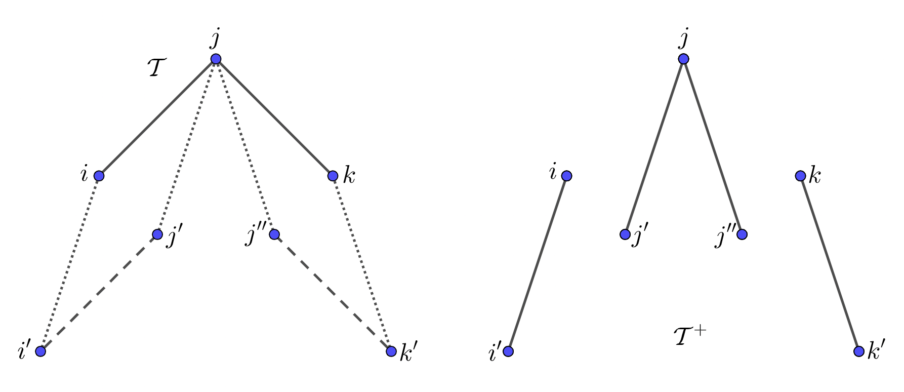
Figure 2: Take 𝒯={𝐢={i,j,k},E={(i,j),(j,k)}}{\mathcal{T}}=\{{\bf i}=\{i,j,k\},E=\{(i,j),(j,k)\}\} to be a forest, then 𝒯+{\mathcal{T}}^{+} constructed in Proposition 3.4 is given by 𝒯+={𝐢+=(i,i′,j,j′,j′′,k,k′),E+={(i,i′),(j,j′),(j,j′′),(k,k′)}}{\mathcal{T}}^{+}=\{{\bf i}^{+}=(i,i^{\prime},j,j^{\prime},j^{\prime\prime},k,k^{\prime}),E^{+}=\{(i,i^{\prime}),(j,j^{\prime}),(j,j^{\prime\prime}),(k,k^{\prime})\}\}.
Example 3.7.

Take 𝒯={𝐢={i,j,k},E={(i,j),(j,k)}}{\mathcal{T}}=\{{\bf i}=\{i,j,k\},E=\{(i,j),(j,k)\}\} to be a forest, which is a path of length two (See Figure 2). It has only one connected component, i.e. θ⁡(𝒯)=1\theta({\mathcal{T}})=1. 𝒜𝒯=Ai​j​Aj​k{\mathcal{A}}_{\mathcal{T}}=A_{ij}A_{jk}. The summation

∑i​j​k∗A𝒯=∑i​j​k​distinctAi​j​Aj​k,\displaystyle\sum_{ijk}^{*}A_{\mathcal{T}}=\sum_{ijk\text{distinct}}A_{ij}A_{jk},

which counts the number of ways to embed 𝒯{\mathcal{T}} to 𝒢{\mathcal{G}}, where vertices of 𝒯{\mathcal{T}} are mapped to distinct vertices [[N]][\![{N}]\!] of 𝒢{\mathcal{G}}. The forest 𝒯+{\mathcal{T}}^{+} constructed in Proposition 3.4 is given by 𝒯+={𝐢+=(i,i′,j,j′,j′′,k,k′),E+={(i,i′),(j,j′),(j,j′′),(k,k′)}}{\mathcal{T}}^{+}=\{{\bf i}^{+}=(i,i^{\prime},j,j^{\prime},j^{\prime\prime},k,k^{\prime}),E^{+}=\{(i,i^{\prime}),(j,j^{\prime}),(j,j^{\prime\prime}),(k,k^{\prime})\}\}, which has three connected components; and i,j,ki,j,k are in different connected components of 𝒯+{\mathcal{T}}^{+}.

Proposition 3.8.

For any graph 𝒯=(𝐢,E){\mathcal{T}}=({\bf i},E), if it is a forest, we have

∑𝐢A𝒯=Nθ⁡(𝒯)​d|E|,\displaystyle\sum_{{\bf i}}A_{{\mathcal{T}}}=N^{\theta({\mathcal{T}})}d^{|E|}, (3.14)

and

1Nθ⁡(𝒯)​d|E|​∑𝐢∗A𝒯=c𝒯+O≺⁡(dN),c𝒯=∏i∈𝐢:deg⁡(i)⩾1(d−1)(d−2)⋯(d−deg(i)+1)d|E|−θ⁡(𝒯)≍1.\displaystyle\begin{split}&\frac{1}{N^{\theta({\mathcal{T}})}d^{|E|}}\sum^{*}_{{\bf i}}A_{{\mathcal{T}}}=c_{{\mathcal{T}}}+\OO_{\prec}\left(\frac{d}{N}\right),\\ &c_{\mathcal{T}}=\frac{\prod_{i\in{\bf i}:\deg(i)\geqslant 1}(d-1)(d-2)\cdots(d-\deg(i)+1)}{d^{|E|-\theta({\mathcal{T}})}}\asymp 1.\end{split} (3.15)

By definition, the numerator of c𝒯c_{\mathcal{T}} is equal to 11 if the deg⁡(i)=1\deg(i)=1. If 𝒯{\mathcal{T}} contains exactly one cycle, then we have

∑𝐢∗A𝒯≺Nθ⁡(𝒯)−1​d|E|.\displaystyle\sum^{*}_{{\bf i}}A_{{\mathcal{T}}}\prec N^{\theta({\mathcal{T}})-1}d^{|E|}. (3.16)
Remark 3.9.

Given a forest 𝒯=(𝐢,E){\mathcal{T}}=({\bf i},E). 𝒯+=(𝐢+,E+){\mathcal{T}}^{+}=({\bf i}^{+},E^{+}) is as constructed in Propositions 3.4 or 3.5. Since 𝒯+{\mathcal{T}}^{+} and 𝒯{\mathcal{T}} have the same degree profile (except for vertices with degree one), we have c𝒯=c𝒯+c_{{\mathcal{T}}}=c_{{\mathcal{T}}^{+}} as in (3.15).

Proof of Proposition 3.4.

Since the row and column sums of AA equal dd, by introducing new indices {je,je′}e∈E\{j_{e},j_{e}^{\prime}\}_{e\in E}, we rewrite the left-hand side of (3.11) as

1Nθ⁡(𝒯)​d|E|​∑𝐢∗𝔼⁡[A𝒯​F𝐢]=1Nθ⁡(𝒯)+|E|​d2​|E|​∑𝐢∗∑𝐣𝔼⁡[A𝒯​∏e∈EAje​je′​F𝐢]=1Nθ⁡(𝒯)+|E|​d2​|E|(∑∗𝐢𝐣𝔼[∏e∈Eχie​ie′je​je′(A)F𝐢]+∑∗𝐢∑𝐣:𝐢𝐣not distinct𝔼[A𝒯∏e∈EAje​je′F𝐢]+∑∗𝐢𝐣𝔼[(A𝒯∏e∈EAje​je′−∏e∈Eχie​ie′je​je′(A))F𝐢]).\displaystyle\begin{split}&\phantom{{}={}}\frac{1}{N^{\theta({\mathcal{T}})}d^{|E|}}\sum^{*}_{{\bf i}}\mathbb{E}\left[A_{{\mathcal{T}}}F_{{\bf i}}\right]=\frac{1}{N^{\theta({\mathcal{T}})+|E|}d^{2|E|}}\sum^{*}_{{\bf i}}\sum_{{\bf j}}\mathbb{E}\left[A_{{\mathcal{T}}}\prod_{e\in E}A_{j_{e}j_{e}^{\prime}}F_{{\bf i}}\right]\\ &=\frac{1}{N^{\theta({\mathcal{T}})+|E|}d^{2|E|}}\left(\sum^{*}_{{\bf i}{\bf j}}\mathbb{E}\left[\prod_{e\in E}\chi_{i_{e}i^{\prime}_{e}}^{j_{e}j^{\prime}_{e}}(A)F_{\bf i}\right]+\sum^{*}_{{\bf i}}\sum_{\begin{subarray}{c}{\bf j}:{\bf i}{\bf j}\\ \text{\rm{not distinct}}\end{subarray}}\mathbb{E}\left[A_{{\mathcal{T}}}\prod_{e\in E}A_{j_{e}j_{e}^{\prime}}F_{\bf i}\right]\right.\\ &\left.+\sum^{*}_{{\bf i}{\bf j}}\mathbb{E}\left[\left(A_{{\mathcal{T}}}\prod_{e\in E}A_{j_{e}j^{\prime}_{e}}-\prod_{e\in E}\chi_{i_{e}i^{\prime}_{e}}^{j_{e}j^{\prime}_{e}}(A)\right)F_{\bf i}\right]\right).\end{split} (3.17)

The second term of the right-hand side in (3.17) can be estimated by

|1Nθ⁡(𝒯)+|E|​d2​|E|∑∗𝐢∑𝐣:𝐢𝐣not distinctA𝒯∏e∈EAje​je′F𝐢(A)|⩽1Nθ⁡(𝒯)+|E|​d2​|E|∑∗𝐢∑𝐣:𝐢𝐣not distinctA𝒯∏e∈EAje​je′𝒞(F,A)⩽1N𝒞(F,A),\displaystyle\begin{split}&\phantom{{}={}}\left|\frac{1}{N^{\theta({\mathcal{T}})+|E|}d^{2|E|}}\sum^{*}_{{\bf i}}\sum_{\begin{subarray}{c}{\bf j}:{\bf i}{\bf j}\\ \text{\rm{not distinct}}\end{subarray}}A_{{\mathcal{T}}}\prod_{e\in E}A_{j_{e}j_{e}^{\prime}}F_{\bf i}(A)\right|\\ &\leqslant\frac{1}{N^{\theta({\mathcal{T}})+|E|}d^{2|E|}}\sum^{*}_{{\bf i}}\sum_{\begin{subarray}{c}{\bf j}:{\bf i}{\bf j}\\ \text{\rm{not distinct}}\end{subarray}}A_{{\mathcal{T}}}\prod_{e\in E}A_{j_{e}j_{e}^{\prime}}\mathcal{C}(F,A)\leqslant\frac{1}{N}\mathcal{C}(F,A),\end{split} (3.18)

where in the last line 𝐢𝐣{\bf i}{\bf j} are not distinct, either some je=je′j_{e}=j_{e}^{\prime} then Aje​je′=0A_{j_{e}j_{e}^{\prime}}=0, or 𝒯∪e∈E{je,je′}{\mathcal{T}}\cup_{e\in E}\{j_{e},j_{e}^{\prime}\} has less than θ⁡(𝒯)+|E|\theta({\mathcal{T}})+|E| connected components. By (3.14), in this case the sum over 𝐢𝐣{\bf i}{\bf j} is bounded by O⁡(Nθ⁡(𝒯)+|E|−1​d2​|E|)\OO(N^{\theta({\mathcal{T}})+|E|-1}d^{2|E|}). Similarly, using |Ai​j​Ak​ℓ−χi​jk​ℓ​(A)|=Ai​j​Ak​ℓ​[Ai​k+Aj​l−Ai​k​Aj​l]⩽Ai​j​Ak​ℓ​[Ai​k+Aj​l]|A_{ij}A_{k\ell}-\chi_{ij}^{k\ell}(A)|=A_{ij}A_{k\ell}[A_{ik}+A_{jl}-A_{ik}A_{jl}]\leqslant A_{ij}A_{k\ell}[A_{ik}+A_{jl}], we also have

|1Nθ⁡(𝒯)+|E|​d2​|E|​∑𝐢𝐣∗[(A𝒯​∏e∈EAje​je′−∏e∈Eχie​ie′je​je′​(A))​F𝐢]|⩽dN​𝒞​(F,A).\displaystyle\left|\frac{1}{N^{\theta({\mathcal{T}})+|E|}d^{2|E|}}\sum^{*}_{\bf ij}\left[\left(A_{{\mathcal{T}}}\prod_{e\in E}A_{j_{e}j^{\prime}_{e}}-\prod_{e\in E}\chi_{i_{e}i^{\prime}_{e}}^{j_{e}j^{\prime}_{e}}(A)\right)F_{\bf i}\right]\right|\leqslant\frac{d}{N}\mathcal{C}(F,A). (3.19)

By plugging the estimates (3.18) and (3.19) into (3.17), we get

1Nθ⁡(𝒯)​d|E|​∑𝐢∗𝔼⁡[A𝒯​F𝐢]=1Nθ⁡(𝒯)+|E|​d2​|E|​∑𝐢𝐣∗𝔼⁡[∏e∈Eχie​ie′je​je′​(A)​F𝐢​(A)]+O⁡(d​𝔼​[𝒞⁡(F,A)]N)=1Nθ⁡(𝒯)+|E|​d2​|E|​∑𝐢𝐣∗𝔼⁡[F⁡(A+∑e∈Eξie​ie′je​je′)​∏e∈Eχie​jeie′​je′​(A)]+O⁡(d​𝔼​[𝒞⁡(F,A)]N),\displaystyle\begin{split}&\phantom{{}={}}\frac{1}{N^{\theta({\mathcal{T}})}d^{|E|}}\sum^{*}_{{\bf i}}\mathbb{E}\left[A_{{\mathcal{T}}}F_{{\bf i}}\right]=\frac{1}{N^{\theta({\mathcal{T}})+|E|}d^{2|E|}}\sum^{*}_{{\bf i}{\bf j}}\mathbb{E}\left[\prod_{e\in E}\chi_{i_{e}i^{\prime}_{e}}^{j_{e}j^{\prime}_{e}}(A)F_{\bf i}(A)\right]+\OO\left(\frac{d\mathbb{E}[\mathcal{C}(F,A)]}{N}\right)\\ &=\frac{1}{N^{\theta({\mathcal{T}})+|E|}d^{2|E|}}\sum^{*}_{\bf ij}\mathbb{E}\left[F\left(A+\sum_{e\in E}\xi_{i_{e}i^{\prime}_{e}}^{j_{e}j^{\prime}_{e}}\right)\prod_{e\in E}\chi_{i_{e}j_{e}}^{i^{\prime}_{e}j^{\prime}_{e}}(A)\right]+\OO\left(\frac{d\mathbb{E}[\mathcal{C}(F,A)]}{N}\right),\end{split} (3.20)

where we used Proposition 3.2 in the last line. By Proposition 3.2 and estimates analogous to the ones above, we have

1N|𝐢|​∑𝐢∗𝔼⁡[F𝐢]=1Nθ⁡(𝒯)+|E|​d2​|E|​∑𝐢∗∑𝐣𝔼⁡[∏e∈EAie​je​Aie′​je′​F𝐢]=1Nθ⁡(𝒯)+|E|​d2​|E|​∑𝐢𝐣∗𝔼⁡[∏e∈Eχie​jeie′​je′​(A)​F𝐢​(A)]+O⁡(d​𝔼​[𝒞⁡(F,A)]N),\displaystyle\begin{split}&\phantom{{}={}}\frac{1}{N^{|{\bf i}|}}\sum^{*}_{{\bf i}}\mathbb{E}\left[F_{{\bf i}}\right]=\frac{1}{N^{\theta({\mathcal{T}})+|E|}d^{2|E|}}\sum^{*}_{{\bf i}}\sum_{{\bf j}}\mathbb{E}\left[\prod_{e\in E}A_{i_{e}j_{e}}A_{i^{\prime}_{e}j_{e}^{\prime}}F_{{\bf i}}\right]\\ &=\frac{1}{N^{\theta({\mathcal{T}})+|E|}d^{2|E|}}\sum^{*}_{{\bf i}{\bf j}}\mathbb{E}\left[\prod_{e\in E}\chi_{i_{e}j_{e}}^{i^{\prime}_{e}j^{\prime}_{e}}(A)F_{\bf i}(A)\right]+\OO\left(\frac{d\mathbb{E}[\mathcal{C}(F,A)]}{N}\right),\end{split} (3.21)

where in the first equality we used (3.14) that 𝒯{\mathcal{T}} is a forest and θ⁡(𝒯)=|𝐢|−|E|\theta({\mathcal{T}})=|{\bf i}|-|E|. The new graph 𝒯+=(𝐢𝐣,E+){\mathcal{T}}^{+}=({\bf i}{\bf j},E^{+}) with E+=∪e∈E{ie,je}∪{ie′,je′}E^{+}=\cup_{e\in E}\{i_{e},j_{e}\}\cup\{i_{e}^{\prime},j_{e}^{\prime}\} has θ⁡(𝒯+)=|𝐢|=|E|+θ⁡(𝒯)\theta({\mathcal{T}}^{+})=|{\bf i}|=|E|+\theta({\mathcal{T}}) connected components, and 2​|E|2|E| edges. The claim now follows from combining (3.20) and (3.21), and replacing ∏e∈Eχie​jeie′​je′​(A)\prod_{e\in E}\chi_{i_{e}j_{e}}^{i^{\prime}_{e}j^{\prime}_{e}}(A) to ∏e∈EAie​je​Aie′​je′=A𝒯+\prod_{e\in E}A_{i_{e}j_{e}}A_{i_{e}^{\prime}j_{e}^{\prime}}=A_{{\mathcal{T}}^{+}}. ∎

Proof of Proposition 3.5.

The two estimates (3.12) and (3.13) can be proven in the same way as for Proposition 3.4, by using (3.4) to do the discrete integration by part. We omit their proofs. ∎

Proof of Proposition 3.8.

In the special case that 𝒯{\mathcal{T}} is a tree, for the sum ∑𝐢A𝒯\sum_{\bf i}A_{{\mathcal{T}}}, we can sequentially sum over leaf vertices. Each gives a factor dd, and the sum over the root vertex gives a factor NN. Thus ∑𝐢A𝒯=N​d|𝐢|−1\sum_{{\bf i}}A_{{\mathcal{T}}}=Nd^{|{\bf i}|-1}. In the general case, when 𝒯{\mathcal{T}} is a forest. We can sum over each of its connected components. There are θ⁡(𝒯)\theta({\mathcal{T}}) connected components, and |E|=|𝐢|−θ⁡(𝒯)|E|=|{\bf i}|-\theta({\mathcal{T}}), so (3.14) follows.

We assume that 𝒯{\mathcal{T}} contains exactly one cycle i1i2⋯iℓi_{1}i_{2}\cdots i_{\ell} of length ℓ\ell, we can sequentially sum over other vertices as in (3.14)

∑∗𝐢A𝒯⩽Nθ⁡(𝒯)−1d|E|−ℓ∑∗i1,i2,⋯,iℓAi1​i2Ai2​i3⋯Aiℓ​i1=Nθ⁡(𝒯)−1d|E|−ℓZ,\displaystyle\sum^{*}_{{\bf i}}A_{{\mathcal{T}}}\leqslant N^{\theta({\mathcal{T}})-1}d^{|E|-\ell}\sum^{*}_{i_{1},i_{2},\cdots,i_{\ell}}A_{i_{1}i_{2}}A_{i_{2}i_{3}}\cdots A_{i_{\ell}i_{1}}=N^{\theta({\mathcal{T}})-1}d^{|E|-\ell}Z, (3.22)

where ZZ counts the number of cycles of length ℓ\ell. To upper bound the righthand side of (3.22), we recall from [51, Theorem 3]: for any finite subgraph 𝒥{\mathcal{J}} with |𝒥||{\mathcal{J}}| edges,

ℙ⁡(𝒥⊂𝒢)=(1+o⁡(1))​(dn)|𝒥|.\displaystyle\mathbb{P}({\mathcal{J}}\subset{\mathcal{G}})=(1+\oo(1))\left(\frac{d}{n}\right)^{|{\mathcal{J}}|}. (3.23)

Using (3.23), for any k⩾1k\geqslant 1, 𝔼⁡[Zk]⩽Ck​dk​ℓ\mathbb{E}[Z^{k}]\leqslant C_{k}d^{k\ell}. It follows by Markov’s inequality

ℙ⁡(Z⩾dℓ​Nε)⩽CkNε​k.\displaystyle\mathbb{P}(Z\geqslant d^{\ell}N^{\varepsilon})\leqslant\frac{C_{k}}{N^{\varepsilon k}}.

We conclude that Z≺dℓZ\prec d^{\ell}, and the claim (3.16) follows from combining with (3.22).

We prove (3.15) by induction. If 𝒯{\mathcal{T}} consists of singletons, i.e. E=∅E=\emptyset, then ∑𝐢∗A𝒯/Nθ⁡(𝒯)=c𝒯=1\sum^{*}_{{\bf i}}A_{{\mathcal{T}}}/N^{\theta({\mathcal{T}})}=c_{{\mathcal{T}}}=1. Otherwise, there exists some vertex ii, such that all of its neighbors are leaf vertices, except possibly one. We can decompose 𝒯{\mathcal{T}} in the following way: 𝒯′=(𝐢′,E′){\mathcal{T}}^{\prime}=({\bf i}^{\prime},E^{\prime}), i∈𝐢′i\in{\bf i}^{\prime} with deg𝒯′⁡(i)⩽1\deg_{{\mathcal{T}}^{\prime}}(i)\leqslant 1 and 𝐢=𝐢′​𝐣,𝐣={j1,j2,⋯,jb}{\bf i}={\bf i}^{\prime}{\bf j},{\bf j}=\{j_{1},j_{2},\cdots,j_{b}\}, E=E′∪{i,j1}∪⋯{i,jb}E=E^{\prime}\cup\{i,j_{1}\}\cup\cdots\{i,j_{b}\}.

∑∗𝐢A𝒯=∑∗𝐢′A𝒯′∑∗𝐣:𝐢′​𝐣​distinctAi​j1Ai​j2⋯Ai​jb.\displaystyle\sum^{*}_{{\bf i}}A_{{\mathcal{T}}}=\sum^{*}_{{\bf i}^{\prime}}A_{{\mathcal{T}}^{\prime}}\sum^{*}_{{\bf j}:{\bf i}^{\prime}{\bf j}\text{ distinct}}A_{ij_{1}}A_{ij_{2}}\cdots A_{ij_{b}}. (3.24)

The two cases that deg𝒯′⁡(i)=0\deg_{{\mathcal{T}}^{\prime}}(i)=0 and deg𝒯′⁡(i)=1\deg_{{\mathcal{T}}^{\prime}}(i)=1 are similar. We will only study the case when deg𝒯′⁡(i)=1\deg_{{\mathcal{T}}^{\prime}}(i)=1. Say Ai​i′=1A_{ii^{\prime}}=1 with i′∈𝐢′i^{\prime}\in{\bf i}^{\prime}, then deg𝒯⁡(i)=b+1\deg_{{\mathcal{T}}}(i)=b+1, and from the definition of c𝒯c_{\mathcal{T}} in (3.15) we obtain

c𝒯=c𝒯′​(d−1)(d−2)⋯(d−b)db.\displaystyle c_{{\mathcal{T}}}=c_{{\mathcal{T}}^{\prime}}\frac{(d-1)(d-2)\cdots(d-b)}{d^{b}}. (3.25)

We enumerate the neighbors of vertex ii in 𝒢{\mathcal{G}} as i′,k1,k2,⋯,kd−1i^{\prime},k_{1},k_{2},\cdots,k_{d-1}. If {k1,k2,⋯,kd−1}∩𝐢′=∅\{k_{1},k_{2},\cdots,k_{d-1}\}\cap{\bf i}^{\prime}=\emptyset, then j1,j2,⋯,jbj_{1},j_{2},\cdots,j_{b} can take any values in k1,k2,⋯,kd−1k_{1},k_{2},\cdots,k_{d-1}, and ∑𝐣:𝐢′​𝐣​distinct∗Ai​j1Ai​j2⋯Ai​jb=(d−1)(d−2)⋯(d−b)\sum^{*}_{{\bf j}:{\bf i}^{\prime}{\bf j}\text{ distinct}}A_{ij_{1}}A_{ij_{2}}\cdots A_{ij_{b}}=(d-1)(d-2)\cdots(d-b). This corresponds to the first term in the following decomposition.

∑𝐢∗A𝒯=∑𝐢∗A𝒯​∏k∈𝐢′∖{i′}(1−Ai​k)+∑𝐢∗A𝒯​(1−∏k∈𝐢′∖{i′}(1−Ai​k)).\displaystyle\sum^{*}_{{\bf i}}A_{{\mathcal{T}}}=\sum^{*}_{{\bf i}}A_{{\mathcal{T}}}\prod_{k\in{\bf i}^{\prime}\setminus\{i^{\prime}\}}(1-A_{ik})+\sum^{*}_{{\bf i}}A_{{\mathcal{T}}}\left(1-\prod_{k\in{\bf i}^{\prime}\setminus\{i^{\prime}\}}(1-A_{ik})\right). (3.26)

For the second term on the righthand side of (3.26), we notice that |1−∏k∈𝐢′∖{i′}(1−Ai​k)|≲∑k∈𝐢′∖{i′}Ai​k\left|1-\prod_{k\in{\bf i}^{\prime}\setminus\{i^{\prime}\}}(1-A_{ik})\right|\lesssim\sum_{k\in{\bf i}^{\prime}\setminus\{i^{\prime}\}}A_{ik}. By adding the edge {i,k}\{i,k\} with k∈𝐢′∖{i′}k\in{\bf i}^{\prime}\setminus\{i^{\prime}\} to 𝒯{\mathcal{T}}, it either forms a cycle or reduces the number of connected component by 11. Thus from the discussing above, using (3.14) and (3.16), we get

∑𝐢∗A𝒯=(d−1)(d−2)⋯(d−b)∑𝐢′∗A𝒯′+O≺(Nθ⁡(𝒯)−1d|E|+1).\displaystyle\sum^{*}_{{\bf i}}A_{{\mathcal{T}}}=(d-1)(d-2)\cdots(d-b)\sum^{*}_{{\bf i}^{\prime}}A_{{\mathcal{T}}^{\prime}}+\OO_{\prec}(N^{\theta({\mathcal{T}})-1}d^{|E|+1}). (3.27)

The statement (3.15) follows from combining (3.25) and (3.27).

∎

4 Green’s Function Estimates

In this section we collect some estimates on the Green’s function GG and the Stieltjes transform of the spectral measure mm. These will be used repeatedly in the rest of the paper. We also introduce monomials in the Green’s function entries, and record some of their basic properties.

By our definition, the Green’s function G=P⟂​(H−z)−1​P⟂G=P_{\perp}(H-z)^{-1}P_{\perp} is symmetric and satisfies (2.2). The Ward identity states that the Green’s function GG satisfies

1N​∑j|Gi​j|2=Im[Gi​i]N​η,1N​∑i​j|Gi​j|2=Im[m]η;\frac{1}{N}\sum_{j}|G_{ij}|^{2}=\frac{\mathop{\mathrm{Im}}[G_{ii}]}{N\eta},\qquad\frac{1}{N}\sum_{ij}|G_{ij}|^{2}=\frac{\mathop{\mathrm{Im}}[m]}{\eta}; (4.1)

We record the following basic result, which follows from Theorem 2.1 and we will use them repeatedly throughout the rest of the paper.

Lemma 4.1.

Fix small 𝔠>0{\mathfrak{c}}>0, suppose that N𝔠⩽d⩽N2/3−𝔠N^{\mathfrak{c}}\leqslant d\leqslant N^{2/3-{\mathfrak{c}}}. With overwhelming probability, uniformly for z∈𝐃z\in\mathbf{D} from (2.8),

maxx≠y⁡|Gx​y​(z)|⩽Λo​(z),maxx​x⁡|Gx​x​(z)|⩽2,max⁡Imx⁡[Gx​x​(z)]≺Im[m⁡(z)],\displaystyle\max_{x\neq y}|G_{xy}(z)|\leqslant\Lambda_{o}(z),\quad\max_{xx}|G_{xx}(z)|\leqslant 2,\quad\max_{x}\mathop{\mathrm{Im}}[G_{xx}(z)]\prec\mathop{\mathrm{Im}}[m(z)], (4.2)

where Λo\Lambda_{o} is from Theorem 2.1.

Proof.

The first two relations in (4.2) follow directly from Theorem 2.1, for the last relation, we use the delocalization of eigenvectors maxα⁡maxi​|uα​(i)|≺1/N,\max_{\alpha}\max_{i}|u_{\alpha}(i)|\prec 1/\sqrt{N}, then

Im[Gx​x]=∑α=2Nuα​(x)2​η|λα−z|2≺1N​∑α=2Nη|λα−z|2=Im[m].\displaystyle\mathop{\mathrm{Im}}[G_{xx}]=\sum_{\alpha=2}^{N}\frac{u_{\alpha}(x)^{2}\eta}{|\lambda_{\alpha}-z|^{2}}\prec\frac{1}{N}\sum_{\alpha=2}^{N}\frac{\eta}{|\lambda_{\alpha}-z|^{2}}=\mathop{\mathrm{Im}}[m].

∎

Remark 4.2.

We recall ξi​jk​ℓ\xi_{ij}^{k\ell} from (3.1). As a consequence of Lemma 4.1, for any fixed b∈ℕb\in\mathbb{N} we find using a resolvent expansion that the following holds with overwhelming probability

maxx​y|Gx​y(A+ξ)|⩽|Gx​y(A)|+O(d−1/2),ξ=∑a=1bξia​jaka​ℓa.\max_{xy}\biggl\lvert G_{xy}(A+\xi)\biggr\rvert\leqslant|G_{xy}(A)|+\OO(d^{-1/2}),\quad\xi=\sum_{a=1}^{b}\xi_{i_{a}j_{a}}^{k_{a}\ell_{a}}.

In the following proposition we collect some estimates on the Stieltjes transform:

Proposition 4.3.

Fix z∈𝐃z\in\mathbf{D} from (2.8). For any derivative operators ∂ξ1,∂ξ2,⋯,∂ξb\partial_{\xi_{1}},\partial_{\xi_{2}},\cdots,\partial_{\xi_{b}} as in Definition 3.3, with ∪a=1b𝐕(ξa)={i,j}∪𝐦\cup_{a=1}^{b}\bm{V}(\xi_{a})=\{i,j\}\cup{\bf m}, let ∂𝛏=∂ξ1∂ξ2,⋯∂ξb\partial_{\bm{\xi}}=\partial_{\xi_{1}}\partial_{\xi_{2}},\cdots\partial_{\xi_{b}}. Then for b⩾1b\geqslant 1 the derivative ∂𝛏m⁡(z)\partial_{\bm{\xi}}m(z) is a sum of terms in the following form

Im[m]N​η​∑𝐤Gi​ja​(z)​X𝐤𝐦​i​(z)​Y𝐤𝐦​j​(z),\displaystyle\frac{\mathop{\mathrm{Im}}[m]}{N\eta}\sum_{{\bf k}}G^{a}_{ij}(z)X_{{\bf k}{\bf m}i}(z)Y_{{\bf k}{\bf m}j}(z), (4.3)

where a⩾0a\geqslant 0, the index set 𝐤=∅{\bf k}=\emptyset and |Xk​𝐦​i​(z)|2,|Yk​𝐦​j​(z)|2=O≺⁡(1)|X_{k{\bf m}i}(z)|^{2},|Y_{k{\bf m}j}(z)|^{2}=\OO_{\prec}(1) or 𝐤={k}{\bf k}=\{k\} and ∑k|Xk​𝐦​i​(z)|2,∑k|Yk​𝐦​j​(z)|2=O≺⁡(1)\sum_{k}|X_{k{\bf m}i}(z)|^{2},\sum_{k}|Y_{k{\bf m}j}(z)|^{2}=\OO_{\prec}(1). It follows that

|∂𝝃m⁡(z)|≺Im[m⁡(z)]N​η.\displaystyle|\partial_{\bm{\xi}}m(z)|\prec\frac{\mathop{\mathrm{Im}}[m(z)]}{N\eta}. (4.4)
Proof.

The derivative ∂𝝃m\partial_{\bm{\xi}}m is a sum of terms in the following form

1N∑kGk​v1Gv2​v3⋯Gv2​b−2​v2​b−1Gv2​b​k,\displaystyle\frac{1}{N}\sum_{k}G_{kv_{1}}G_{v_{2}v_{3}}\cdots G_{v_{2b-2}v_{2b-1}}G_{v_{2b}k}, (4.5)

where v1,v2,⋯,v2​b∈i​j​𝐦v_{1},v_{2},\cdots,v_{2b}\in ij{\bf m}. For the Green’s function entries in (4.5) we can regroup them depending if they contain indices i,ji,j

1N​∑k=1NGi​ja​X~k​𝐦​i​Y~k​𝐦​j,\displaystyle\frac{1}{N}\sum_{k=1}^{N}G_{ij}^{a}\tilde{X}_{k{\bf m}i}\tilde{Y}_{k{\bf m}j},

where for each Gx​yG_{xy} in (4.5), if the index set {x,y}\{x,y\} only contains ii we put it in X~k​𝐦​i\tilde{X}_{k{\bf m}i}; if it only contains jj we put it in Y~k​𝐦​j\tilde{Y}_{k{\bf m}j}; if it does not contain i,ji,j we still put it in X~k​𝐦​j\tilde{X}_{k{\bf m}j}.

There are two cases. In the first case, each of X~k​𝐦​i,Y~k​𝐦​j\tilde{X}_{k{\bf m}i},\tilde{Y}_{k{\bf m}j} contains one of Gk​v1,Gv2​b​kG_{kv_{1}},G_{v_{2b}k}; in the second case, both Gk​v1,Gv2​b​kG_{kv_{1}},G_{v_{2b}k} are in X~k​𝐦​i\tilde{X}_{k{\bf m}i} or Y~k​𝐦​j\tilde{Y}_{k{\bf m}j}.

In the first case, say Gk​v1G_{kv_{1}} is in X~k​𝒎​i\tilde{X}_{k\bm{m}i}, using |Gvs​vs+1|≺1|G_{v_{s}v_{s+1}}|\prec 1 from Lemma 4.1 and Ward identity (4.1) we have

∑k=1N|X~k​𝐦​i|2≺∑k=1N|Gk​v1|2≺Im[m]η,∑k=1N|Y~k​𝐦​j|2≺∑k=1N|Gk​v2​b|2≺Im[m]η.\displaystyle\sum_{k=1}^{N}|\tilde{X}_{k{\bf m}i}|^{2}\prec\sum_{k=1}^{N}|G_{kv_{1}}|^{2}\prec\frac{\mathop{\mathrm{Im}}[m]}{\eta},\quad\sum_{k=1}^{N}|\tilde{Y}_{k{\bf m}j}|^{2}\prec\sum_{k=1}^{N}|G_{kv_{2b}}|^{2}\prec\frac{\mathop{\mathrm{Im}}[m]}{\eta}.

The claim (4.3) follows by taking 𝐤={k}{\bf k}=\{k\}, Im[m]/η​X𝐤𝐦​i=X~k​𝐦​i,Im[m]/η​Y𝐤𝐦​j=Y~k​𝐦​j\sqrt{\mathop{\mathrm{Im}}[m]/\eta}X_{{\bf k}{\bf m}i}=\tilde{X}_{k{\bf m}i},\sqrt{\mathop{\mathrm{Im}}[m]/\eta}Y_{{\bf k}{\bf m}j}=\tilde{Y}_{k{\bf m}j}.

In the second case, say both Gk​v1,Gv2​b​kG_{kv_{1}},G_{v_{2b}k} are in X~k​𝐦​i\tilde{X}_{k{\bf m}i}. Then Y~k​𝐦​j=Y~𝐦​j\tilde{Y}_{k{\bf m}j}=\tilde{Y}_{{\bf m}j} does not depend on the index kk. Moreover, using |Gvs​vs+1|≺1|G_{v_{s}v_{s+1}}|\prec 1 from Lemma 4.1 and Ward identity (4.1)

|∑kX~k​𝐦​i|≺∑k=1N|Gk​v1​Gv2​b​k|⩽12​∑k=1N|Gk​v1|2+|Gv2​b​k|2≺Im[m]η.\displaystyle\left|\sum_{k}\tilde{X}_{k{\bf m}i}\right|\prec\sum_{k=1}^{N}|G_{kv_{1}}G_{v_{2b}k}|\leqslant\frac{1}{2}\sum_{k=1}^{N}|G_{kv_{1}}|^{2}+|G_{v_{2b}k}|^{2}\prec\frac{\mathop{\mathrm{Im}}[m]}{\eta}.

The claim (4.3) follows by taking 𝐤=∅{\bf k}=\emptyset, (Im[m]/η)​X𝐤𝐦​i=∑kX~k​𝐦​i,Y𝐤𝐦​j=Y~𝐦​j(\mathop{\mathrm{Im}}[m]/\eta)X_{{\bf k}{\bf m}i}=\sum_{k}\tilde{X}_{k{\bf m}i},Y_{{\bf k}{\bf m}j}=\tilde{Y}_{{\bf m}j}. This finishes the proof of (4.3). The bound (4.4) follows from the decomposition (4.3).

∎

A central object in our proof is the following notion of a polynomial in the Green’s function entries.

Definition 4.4.

Let R=R⁡({xs​t}s,t=1r,y)R=R(\{x_{st}\}_{s,t=1}^{r},y) be a monomial in the r2+1r^{2}+1 abstract variables {xs​t}s,t=1r,y\{x_{st}\}_{s,t=1}^{r},y. We denote its degree by deg⁡(R)\deg(R). For 𝐢∈[[N]]r{\bf i}\in[\![{N}]\!]^{r}, we define its evaluation on the Green’s function and the Stieltjes transform by

R𝐢=R⁡({Gis​it}s,t=1r,m),R_{\bf i}=R(\{G_{i_{s}i_{t}}\}_{s,t=1}^{r},m),

and say that R𝐢R_{\bf i} is a monomial in the Green’s function entries {Gis​it}s,t=1r\{G_{i_{s}i_{t}}\}_{s,t=1}^{r}. We denote the number of off-diagonal entries in R𝐢R_{\bf i} as χ⁡(R𝐢)\chi(R_{\bf i}).

5 Self-Consistent Equation

In this section we construct the self-consistent equation for the Stieltjes transform mm, and prove that the self-consistent equation holds with overwhelming probability.

Proposition 5.1.

Assume N𝔠⩽d⩽N1/3−𝔠N^{\mathfrak{c}}\leqslant d\leqslant N^{1/3-{\mathfrak{c}}}. There exists a finite degree polynomial, depending on dd but not NN,

P⁡(z,u)=1+z​u+u2+Q⁡(u),\displaystyle P(z,u)=1+zu+u^{2}+Q(u), (5.1)

where

Q⁡(u)=a2​u2+a3​u3+a4​u4+⋯+an​un,\displaystyle Q(u)=a_{2}u^{2}+a_{3}u^{3}+a_{4}u^{4}+\cdots+a_{n}u^{n}, (5.2)

is a polynomial with bounded coefficients a2,a3,…,an=O⁡(1/d)a_{2},a_{3},\dots,a_{n}=\OO(1/\sqrt{d}) such that, for any z∈𝐃z\in\mathbf{D} from (2.8)

𝔼⁡[|P⁡(z,m⁡(z))|2​q]≺𝔼⁡[Φq​(z)].\displaystyle\mathbb{E}[|P(z,m(z))|^{2q}]\prec\mathbb{E}[\Phi_{q}(z)]. (5.3)

where the control parameter Φq​(z)\Phi_{q}(z) is defined as

Φq​(z):=d3/2​Λo​(z)N​|P⁡(z,m⁡(z))|2​q−1+∑s=12​q(Im[m⁡(z)]N​η)s​|P⁡(z,m⁡(z))|2​q−s+∑s=12​q−1(1N​η+d3/2​Λo​(z)N)(Im[m⁡(z)]​|∂2P⁡(z,m⁡(z))|N​η)s|P(z,m(z))|2​q−s−1.\displaystyle\begin{split}\Phi_{q}(z):&=\frac{d^{3/2}\Lambda_{o}(z)}{N}|P(z,m(z))|^{2q-1}+\sum_{s=1}^{2q}\left(\frac{\mathop{\mathrm{Im}}[m(z)]}{N\eta}\right)^{s}|P(z,m(z))|^{2q-s}\\ &+\sum_{s=1}^{2q-1}\left(\frac{1}{N\eta}+\frac{d^{3/2}\Lambda_{o}(z)}{N}\right)\left(\frac{\mathop{\mathrm{Im}}[m(z)]|\partial_{2}P(z,m(z))|}{N\eta}\right)^{s}|P(z,m(z))|^{2q-s-1}.\end{split} (5.4)

We will show that the estimate (5.3) results from the switching invariance of random regular graphs. It may be viewed as an approximate Schwinger–Dyson Equation for the random regular graph ensemble; in statistical mechanics and field theory, such equations are typically derived by integration by parts. In the rest of the paper, we write ∂2P⁡(z,w):=∂wP⁡(z,w)\partial_{2}P(z,w)\mathrel{\mathop{:}}=\partial_{w}P(z,w).

Starting from (2.1) and noticing Ai​i=0A_{ii}=0 we obtain

1+z​m=∑i​j∗Ai​j​Gi​jN​(d−1)1/2+1N.1+zm=\sum^{*}_{ij}\frac{A_{ij}G_{ij}}{N(d-1)^{1/2}}+\frac{1}{N}.

By multiplying both sides by Pq−1​P¯qP^{q-1}\bar{P}^{q}, we get

𝔼⁡[(1+z​m)​Pq−1​P¯q]=1N​(d−1)1/2​∑i​j∗𝔼⁡[Ai​j​(Gi​j​Pq−1​P¯q)]+O≺⁡(𝔼⁡[Φq])=d(d−1)1/2​1Nθ⁡(𝒯0)​d|E0|​∑i​j∗𝔼⁡[A𝒯0​R𝐢0​Pq−1​P¯q]+O≺⁡(𝔼⁡[Φq]),\displaystyle\begin{split}\mathbb{E}[(1+zm)P^{q-1}\bar{P}^{q}]&=\frac{1}{N(d-1)^{1/2}}\sum_{ij}^{*}\mathbb{E}[A_{ij}(G_{ij}P^{q-1}\bar{P}^{q})]+\OO_{\prec}(\mathbb{E}[\Phi_{q}])\\ &=\frac{d}{(d-1)^{1/2}}\frac{1}{N^{\theta({\mathcal{T}}_{0})}d^{|E_{0}|}}\sum_{ij}^{*}\mathbb{E}[A_{{\mathcal{T}}_{0}}R_{{\bf i}_{0}}P^{q-1}\bar{P}^{q}]+\OO_{\prec}(\mathbb{E}[\Phi_{q}]),\end{split} (5.5)

where 𝒯0=(𝐢0=i​j,E0={i,j}){\mathcal{T}}_{0}=({\bf i}_{0}={ij},E_{0}=\{i,j\}), A𝒯0=Ai​jA_{{\mathcal{T}}_{0}}=A_{ij} and R𝐢0=Gi​jR_{{\bf i}_{0}}=G_{ij}.

In Sections 5.1 and 5.2, we will show that we can use Propositions 3.4 and 3.5 to further expand (5.5). In this way, starting from the graph 𝒯0=(𝐢0=i​j,E0={i,j}){\mathcal{T}}_{0}=({\bf i}_{0}={ij},E_{0}=\{i,j\}), we will obtain a sequence of graphs

𝒯0=(𝐢0,E0),𝒯1=(𝐢1,E1),𝒯2=(𝐢2,E2),⋯,\displaystyle{\mathcal{T}}_{0}=({\bf i}_{0},E_{0}),\quad{\mathcal{T}}_{1}=({\bf i}_{1},E_{1}),\quad{\mathcal{T}}_{2}=({\bf i}_{2},E_{2}),\quad\cdots,

After we construct graph 𝒯r{\mathcal{T}}_{r}, we need to further use Propositions 3.4 and 3.5 to expand terms in the following form

1d𝔥/2​1Nθ⁡(𝒯r)​d|Er|​∑𝐢r∗𝔼⁡[A𝒯r​R𝐢r​U𝐢r],\displaystyle\begin{split}\frac{1}{d^{{\mathfrak{h}}/2}}\frac{1}{N^{\theta({\mathcal{T}}_{r})}d^{|E_{r}|}}\sum^{*}_{{\bf i}_{r}}\mathbb{E}\left[A_{{\mathcal{T}}_{r}}R_{{\bf i}_{r}}U_{{\bf i}_{r}}\right],\end{split}

where R𝐢rR_{{\bf i}_{r}} is a monomial of Green’s function entries as in Definition 4.4, and U𝐢rU_{{\bf i}_{r}} is in the following form.

Definition 5.2.

Given an index set 𝐢{\bf i}, we will use U𝐢=U𝐢​(m,m¯)U_{\bf i}=U_{\bf i}(m,\bar{m}) to represent an expression in the following form: for fixed b∈ℕb\in\mathbb{N} and discrete derivative operators Dξ1,Dξ2,⋯,DξbD_{\xi_{1}},D_{\xi_{2}},\cdots,D_{\xi_{b}} as in Definition 3.3 with 𝐕⁡(ξ1),𝐕⁡(ξ2),⋯,𝐕⁡(ξb)⊂𝐢\bm{V}(\xi_{1}),\bm{V}(\xi_{2}),\cdots,\bm{V}(\xi_{b})\subset{\bf i},

(∏a=1b(1+Dξa)ea​(d−1​Dξa)1−ea)​Pq−1​P¯q,e1,e2,⋯,eb∈{0,1}.\displaystyle\left(\prod_{a=1}^{b}(1+D_{\xi_{a}})^{e_{a}}(\sqrt{d-1}D_{\xi_{a}})^{1-e_{a}}\right)P^{q-1}\bar{P}^{q},\quad e_{1},e_{2},\cdots,e_{b}\in\{0,1\}. (5.6)

If b=0b=0, then the above expression reduces to Pq−1​P¯qP^{q-1}\bar{P}^{q}.

We remark that from the Taylor expansion (3.9), up to negligible error, U𝐢U_{\bf i} is a finite linear combination of terms in the form ∂𝝃(Pq−1​P¯q)\partial_{\bm{\xi}}(P^{q-1}\bar{P}^{q}).

5.1 Proof of Proposition 5.1

We recall the discussion from last section, that we need to estimate terms in the following form:

Definition 5.3.

For 𝔥,𝔬∈ℕ{\mathfrak{h}},{\mathfrak{o}}\in\mathbb{N}, we use the symbol ℰ𝔥,𝔬{\mathcal{E}}_{{\mathfrak{h}},{\mathfrak{o}}} to denote a finite linear combination of terms of the form for some 𝔥⩾0{\mathfrak{h}}\geqslant 0,

1d𝔥/2​1Nθ⁡(𝒯)​d|E|​∑𝐢∗𝔼⁡[A𝒯​R𝐢​U𝐢],\displaystyle\frac{1}{d^{{\mathfrak{h}}/2}}\frac{1}{N^{\theta({\mathcal{T}})}d^{|E|}}\sum^{*}_{\bf i}\mathbb{E}\left[A_{{\mathcal{T}}}R_{{\bf i}}U_{\bf i}\right], (5.7)

where the forest 𝒯=(𝐢,E){\mathcal{T}}=({\bf i},E) is as in Definition 3.1, R𝐢R_{\bf i} is a monomial of Green’s function entries as in Definition 4.4, such that χ⁡(R𝐢)=𝔬\chi(R_{\bf i})={\mathfrak{o}} (recall that χ⁡(R𝐢)\chi(R_{\bf i}) counts the number of off-diagonal Green’s function entries), and U𝐢U_{\bf i} is as in (5.6).

In the next two propositions, we collect some useful estimates. Their proofs are given by Sections 5.2 and 5.3.

Proposition 5.4.

We adopt assumptions in Proposition 5.1, and recall the polynomial PP from (5.1). For ∂𝛏=∂ξ1∂ξ2,⋯∂ξb\partial_{\bm{\xi}}=\partial_{\xi_{1}}\partial_{\xi_{2}},\cdots\partial_{\xi_{b}} as in Definition (3.3), then for b⩾1b\geqslant 1

∂𝝃P⁡(z,m)=∂𝝃m​∂2P⁡(z,m)+𝒪≺​(Im[m]2(N​η)2)=O≺⁡(Im[m]​|∂2P⁡(z,m)|N​η+Im[m]2(N​η)2),\displaystyle\partial_{\bm{\xi}}P(z,m)=\partial_{\bm{\xi}}m\partial_{2}P(z,m)+\mathcal{O}_{\prec}\left(\frac{\mathop{\mathrm{Im}}[m]^{2}}{(N\eta)^{2}}\right)=\OO_{\prec}\left(\frac{\mathop{\mathrm{Im}}[m]|\partial_{2}P(z,m)|}{N\eta}+\frac{\mathop{\mathrm{Im}}[m]^{2}}{(N\eta)^{2}}\right), (5.8)

and

(d3/2​ΛoN+1N​η)​∂𝝃(Pq−1​(z,m)​P¯q​(z,m))≺Φq.\displaystyle\left(\frac{d^{3/2}\Lambda_{o}}{N}+\frac{1}{N\eta}\right)\partial_{\bm{\xi}}(P^{q-1}(z,m)\bar{P}^{q}(z,m))\prec\Phi_{q}. (5.9)

As a consequence, if R𝐢,U𝐢R_{\bf i},U_{\bf i} are as in Definitions 4.4 and 5.2, then if R𝐢R_{{\bf i}} contains at least one off-diagonal Green’s function entry

(d3/2​ΛoN+Im[m]N​η)​|R𝐢​U𝐢​(A+∑a=1bξa)|≲Φq,\displaystyle\left(\frac{d^{3/2}\Lambda_{o}}{N}+\frac{\mathop{\mathrm{Im}}[m]}{N\eta}\right)\left|R_{\bf i}U_{\bf i}\left(A+\sum_{a=1}^{b}\xi_{a}\right)\right|\lesssim\Phi_{q}, (5.10)

and for 𝔬+𝔥{\mathfrak{o}}+{\mathfrak{h}} large enough such that Λo𝔬+𝔥⩽1/N\Lambda_{o}^{{\mathfrak{o}}+{\mathfrak{h}}}\leqslant 1/N (recall Λo\Lambda_{o} from (2.9)), we have

ℰ𝔥,𝔬≲𝔼⁡[Φq].\displaystyle{\mathcal{E}}_{{\mathfrak{h}},{\mathfrak{o}}}\lesssim\mathbb{E}[\Phi_{q}]. (5.11)
Proposition 5.5.

We assume assumptions in Proposition 5.1. Given a forest 𝒯=(𝐢,E){\mathcal{T}}=({\bf i},E) as in Definition 3.1, R𝐢R_{\bf i} is a monomial of Green’s function entries as in Definition 4.4. Let ∂𝛏=∂ξ1∂ξ2,⋯∂ξb\partial_{\bm{\xi}}=\partial_{\xi_{1}}\partial_{\xi_{2}},\cdots\partial_{\xi_{b}} as in Definition 3.3 with 𝐕⁡(𝛏)⊂𝐢\bm{V}(\bm{\xi})\subset{\bf i}. If R𝐢R_{\bf i} contains at least one off-diagonal Green’s function entry, i.e. R𝐢=Gi​j​R𝐢′R_{\bf i}=G_{ij}R^{\prime}_{{\bf i}}, and i,j∈𝐢i,j\in{\bf i} are in different connected components of 𝒯{\mathcal{T}} then

1Nθ⁡(𝒯)​d|E|​∑𝐢∗𝔼⁡[A𝒯​R𝐢​∂𝝃(Pq−1​P¯q)]≺𝔼⁡[Φq],\displaystyle\frac{1}{N^{\theta({\mathcal{T}})}d^{|E|}}\sum^{*}_{{\bf i}}\mathbb{E}\left[A_{{\mathcal{T}}}R_{{\bf i}}\partial_{\bm{\xi}}(P^{q-1}\bar{P}^{q})\right]\prec\mathbb{E}[\Phi_{q}], (5.12)

In particular, if we take 𝒯=(𝐢,E=∅){\mathcal{T}}=({\bf i},E=\emptyset) then 𝒜𝒯=1{\mathcal{A}}_{{\mathcal{T}}}=1 and

1N|𝐢|​∑𝐢∗𝔼⁡[R𝐢​∂𝝃(Pq−1​P¯q)]≺𝔼⁡[Φq].\displaystyle\frac{1}{N^{|{\bf i}|}}\sum^{*}_{{\bf i}}\mathbb{E}\left[R_{{\bf i}}\partial_{\bm{\xi}}(P^{q-1}\bar{P}^{q})\right]\prec\mathbb{E}[\Phi_{q}]. (5.13)

The following two propositions state how to further expand the expression (5.7) using Propositions 3.4 and 3.5. There are two cases depending if R𝐢R_{{\bf i}} contains off-diagonal Green’s function entry or not. Their proofs are given in Sections 5.4 and 5.5.

Proposition 5.6 (off-diagonal discrete integration by parts).

If R𝐢R_{{\bf i}} in (5.7) contains at least one off-diagonal Green’s function entries, i.e. 𝔬⩾1{\mathfrak{o}}\geqslant 1, then up to small error O≺(d−𝔥/2𝔼[Φq])\OO_{\prec}(d^{-{\mathfrak{h}}/2}\mathbb{E}[\Phi_{q}]), (5.7) is a finite sum of terms in the form

1d𝔥~/2​1Nθ⁡(𝒯+)​d|E+|​∑𝐢+∗𝔼⁡[A𝒯+​R𝐢+​U𝐢+]∈ℰ𝔥~,𝔬~,U𝐢+=(1+D𝒯+)​U𝐢,\displaystyle\frac{1}{d^{\tilde{\mathfrak{h}}/2}}\frac{1}{N^{\theta({\mathcal{T}}^{+})}d^{|E^{+}|}}\sum^{*}_{{\bf i}^{+}}\mathbb{E}\left[A_{{\mathcal{T}}^{+}}R_{{\bf i}^{+}}U_{{\bf i}^{+}}\right]\in{\mathcal{E}}_{\tilde{\mathfrak{h}},\tilde{\mathfrak{o}}},\quad U_{{\bf i}^{+}}=(1+D_{{\mathcal{T}}^{+}})U_{\bf i}, (5.14)

where 𝒯+=(𝐢+,E+){\mathcal{T}}^{+}=({\bf i}^{+},E^{+}) with 𝐢+=𝐢𝐣{\bf i}^{+}={\bf i}{\bf j}, E+=∪e∈E{ie,je}∪{ie′,je′}E^{+}=\cup_{e\in E}\{i_{e},j_{e}\}\cup\{i_{e}^{\prime},j_{e}^{\prime}\}, 𝔥~⩾𝔥+𝔬\tilde{\mathfrak{h}}\geqslant{\mathfrak{h}}+{\mathfrak{o}}.

Proposition 5.7 (diagonal discrete integration by parts).

If R𝐢R_{{\bf i}} in (5.7) is a monomial of diagonal Green’s function entries and mm (𝔬=0{\mathfrak{o}}=0), and contains at least one diagonal Green’s function entry, say R𝐢=Gi​i​R𝐢′R_{{\bf i}}=G_{ii}R^{\prime}_{{\bf i}}, then up to small error O≺(d−𝔥/2𝔼[Φq])\OO_{\prec}(d^{-{\mathfrak{h}}/2}\mathbb{E}[\Phi_{q}]), (5.7) equals

1d𝔥/2​1Nθ⁡(𝒯)​d|E|​∑𝐢∗𝔼⁡[A𝒯​(m​R𝐢′)​U𝐢],\displaystyle\frac{1}{d^{{\mathfrak{h}}/2}}\frac{1}{N^{\theta({\mathcal{T}})}d^{|E|}}\sum^{*}_{{\bf i}}\mathbb{E}\left[A_{{\mathcal{T}}}(mR^{\prime}_{{\bf i}})U_{\bf i}\right],

plus a finite sum of terms in the form

1d𝔥~/2​1Nθ⁡(𝒯+)​d|E+|​∑𝐢+∗𝔼⁡[A𝒯+​R𝐢+​U𝐢+]∈ℰ𝔥~,𝔬~,\displaystyle\frac{1}{d^{\tilde{\mathfrak{h}}/2}}\frac{1}{N^{\theta({\mathcal{T}}^{+})}d^{|E^{+}|}}\sum^{*}_{{\bf i}^{+}}\mathbb{E}\left[A_{{\mathcal{T}}^{+}}R_{{\bf i}^{+}}U_{{\bf i}^{+}}\right]\in{\mathcal{E}}_{\tilde{\mathfrak{h}},\tilde{\mathfrak{o}}}, (5.15)

where there are three cases

  1. 1.

    𝒯+=(j​k​ℓ​m​𝐢,E∪{j,ℓ}∪{k,m}){\mathcal{T}}^{+}=(jk\ell m{\bf i},E\cup\{j,\ell\}\cup\{k,m\}), U𝐢+=(1+Dj​kℓ​m)​U𝐢U_{{\bf i}^{+}}=(1+D_{jk}^{\ell m})U_{{\bf i}} or U𝐢+=d−1​Dj​kℓ​m​U𝐢U_{{\bf i}^{+}}=\sqrt{d-1}D_{jk}^{\ell m}U_{{\bf i}}; then either 𝔥~⩾𝔥+1\tilde{\mathfrak{h}}\geqslant{\mathfrak{h}}+1 or 𝔥~=𝔥\tilde{\mathfrak{h}}={\mathfrak{h}} and 𝔬~⩾1\tilde{\mathfrak{o}}\geqslant 1.

  2. 2.

    𝒯+=(k​ℓ​m​𝐢,E∪{i,ℓ}∪{k,m}){\mathcal{T}}^{+}=(k\ell m{\bf i},E\cup\{i,\ell\}\cup\{k,m\}), where i∈𝐢i\in{\bf i}, U𝐢+=(1+Di​kℓ​m)​U𝐢U_{{\bf i}^{+}}=(1+D_{ik}^{\ell m})U_{{\bf i}} or U𝐢+=d−1​Di​kℓ​m​U𝐢U_{{\bf i}^{+}}=\sqrt{d-1}D_{ik}^{\ell m}U_{{\bf i}}; then either 𝔥~⩾𝔥+1\tilde{\mathfrak{h}}\geqslant{\mathfrak{h}}+1 or 𝔥~=𝔥\tilde{\mathfrak{h}}={\mathfrak{h}} and 𝔬~⩾1\tilde{\mathfrak{o}}\geqslant 1.

  3. 3.

    𝒯+=𝒯{\mathcal{T}}^{+}={\mathcal{T}}, U𝐢+=U𝐢U_{{\bf i}^{+}}=U_{{\bf i}}; then either 𝔥~⩾𝔥+1\tilde{\mathfrak{h}}\geqslant{\mathfrak{h}}+1.

In all three cases 𝔥~+𝔬~⩾𝔥+𝔬+1\tilde{\mathfrak{h}}+\tilde{\mathfrak{o}}\geqslant{\mathfrak{h}}+{\mathfrak{o}}+1.

Starting from the graph 𝒯0=(𝐢0=i​j,E0={i,j}){\mathcal{T}}_{0}=({\bf i}_{0}={ij},E_{0}=\{i,j\}) as in (5.5), using Proposition 3.4 with F𝐢=Gi​j​Pq−1​P¯q−1F_{{\bf i}}=G_{ij}P^{q-1}\bar{P}^{q-1}, we get 𝒯1=(𝐢1=i​j​k​ℓ,E1={i,k}∪{j,ℓ}){\mathcal{T}}_{1}=({\bf i}_{1}=ijk\ell,E_{1}=\{i,k\}\cup\{j,\ell\}). Then for i≠ji\neq j, |F𝐢|≺Λo​|P|2​q−1|F_{\bf i}|\prec\Lambda_{o}|P|^{2q-1}, d3/2​𝒞​(F,A)/N≺Φqd^{3/2}{\mathcal{C}}(F,A)/N\prec\Phi_{q}, and (5.5) equals

d(d−1)1/2​1N2​∑i​j∗𝔼⁡[Gi​j​Pq−1​P¯q]+d(d−1)1/2​1Nθ⁡(𝒯1)​d|E1|​∑i​j​k​ℓ∗𝔼⁡[A𝒯1​Di​jk​ℓ​(Gi​j​Pq−1​P¯q)],\displaystyle\begin{split}&\phantom{{}={}}\frac{d}{(d-1)^{1/2}}\frac{1}{N^{2}}\sum_{ij}^{*}\mathbb{E}[G_{ij}P^{q-1}\bar{P}^{q}]+\frac{d}{(d-1)^{1/2}}\frac{1}{N^{\theta({\mathcal{T}}_{1})}d^{|E_{1}|}}\sum_{ijk\ell}^{*}\mathbb{E}[A_{{\mathcal{T}}_{1}}D_{ij}^{k\ell}(G_{ij}P^{q-1}\bar{P}^{q})],\end{split} (5.16)

with an error bounded by O≺⁡(𝔼⁡[Φq])\OO_{\prec}(\mathbb{E}[\Phi_{q}]). For the first term in (5.16), we have ∑i​jGi​j=0\sum_{ij}G_{ij}=0 and ∑i​j∗Gi​j≺N\sum^{*}_{ij}G_{ij}\prec N. Thus it is bounded by 𝔼⁡[Φq]\mathbb{E}[\Phi_{q}]. For the second term in (5.16), by the discrete chain rule, we can rewrite it as

dd−1​1Nθ⁡(𝒯1)​d|E1|​∑i​j​k​ℓ∗𝔼⁡[A𝒯1​Gi​j​d−1​Di​jk​ℓ​(Pq−1​P¯q)]+d(d−1)1/21Nθ⁡(𝒯1)​d|E1|∑i​j​k​ℓ∗𝔼[A𝒯1Di​jk​ℓ(Gi​j)(1+Di​jk​ℓ)Pq−1P¯q)]+O≺(𝔼[Φq]).\displaystyle\begin{split}&\phantom{{}={}}\frac{d}{d-1}\frac{1}{N^{\theta({\mathcal{T}}_{1})}d^{|E_{1}|}}\sum_{ijk\ell}^{*}\mathbb{E}[A_{{\mathcal{T}}_{1}}G_{ij}\sqrt{d-1}D_{ij}^{k\ell}(P^{q-1}\bar{P}^{q})]\\ &+\frac{d}{(d-1)^{1/2}}\frac{1}{N^{\theta({\mathcal{T}}_{1})}d^{|E_{1}|}}\sum_{ijk\ell}^{*}\mathbb{E}[A_{{\mathcal{T}}_{1}}D_{ij}^{k\ell}(G_{ij})(1+D_{ij}^{k\ell})P^{q-1}\bar{P}^{q})]+\OO_{\prec}(\mathbb{E}[\Phi_{q}]).\end{split} (5.17)

For the first term in (5.17), we recall 𝒯1=({i,j,k,ℓ},{{i,k},{j,ℓ}}){\mathcal{T}}_{1}=(\{i,j,k,\ell\},\{\{i,k\},\{j,\ell\}\}). We notice that i,ji,j are in different connected components of 𝒯1{\mathcal{T}}_{1}. We can Taylor expand d−1​Di​jk​ℓ​(Pq−1​P¯q)\sqrt{d-1}D_{ij}^{k\ell}(P^{q-1}\bar{P}^{q}) as in (3.9), then it is a linear combination of terms in the form ∂𝝃(Pq−1​P¯q)\partial_{\bm{\xi}}(P^{q-1}\bar{P}^{q}). We conclude from (5.12) that the first term in (5.17) is bounded by 𝔼⁡[Φq]\mathbb{E}[\Phi_{q}]. For the second term in (5.17), we can similarly Taylor expand Di​jk​ℓ​Gi​jD_{ij}^{k\ell}G_{ij},

Di​jk​ℓ​Gi​j=∑n=1𝔟−1∂ξnGi​jn!​(d−1)n/2+∂ξ𝔟Gi​j​(A+θ​ξ)𝔟!​(d−1)𝔟/2,ξ=ξi​jk​ℓ.\displaystyle D_{ij}^{k\ell}G_{ij}=\sum_{n=1}^{{\mathfrak{b}}-1}\frac{\partial_{\xi}^{n}G_{ij}}{n!(d-1)^{n/2}}+\frac{\partial_{\xi}^{{\mathfrak{b}}}G_{ij}(A+\theta\xi)}{{\mathfrak{b}}!(d-1)^{{\mathfrak{b}}/2}},\quad\xi=\xi_{ij}^{k\ell}. (5.18)

We notice that ∂ξnGi​j\partial_{\xi}^{n}G_{ij} is a linear combination of monomials of Green’s function entries, and is stochastically bounded, i.e. O≺⁡(1)\OO_{\prec}(1). We can take 𝔟{\mathfrak{b}} large enough such that the remainder term is bounded by O≺⁡(1/N)\OO_{\prec}(1/N). In this way, up to error 𝔼⁡[Φq]\mathbb{E}[\Phi_{q}], the second term in (5.17) can be rewritten as a linear combination of

1d𝔥/2​1Nθ⁡(𝒯1)​d|E1|​∑𝐢1∗𝔼⁡[A𝒯1​R𝐢1​U𝐢1],U𝐢1=Pq−1​P¯q​or ​U𝐢1=d−1​Di​jk​ℓ​Pq−1​P¯q,\displaystyle\frac{1}{d^{{\mathfrak{h}}/2}}\frac{1}{N^{\theta({\mathcal{T}}_{1})}d^{|E_{1}|}}\sum^{*}_{{\bf i}_{1}}\mathbb{E}\left[A_{{\mathcal{T}}_{1}}R_{{\bf i}_{1}}U_{{\bf i}_{1}}\right],\quad U_{{{\bf i}}_{1}}=P^{q-1}\bar{P}^{q}\text{ or }U_{{\bf i}_{1}}=\sqrt{d-1}D_{ij}^{k\ell}P^{q-1}\bar{P}^{q}, (5.19)

with 𝔥⩾0{\mathfrak{h}}\geqslant 0. The terms corresponding to 𝔥=0{\mathfrak{h}}=0 are from taking n=1n=1 in (5.18), and U𝐢1=Pq−1​P¯qU_{{\bf i}_{1}}=P^{q-1}\bar{P}^{q}:

dd−11Nθ⁡(𝒯1)​d|E1|∑i​j​k​ℓ∗𝔼[Ai​kAj​ℓ∂i​jk​ℓ(Gi​j)Pq−1P¯q)]=−dd−11Nθ⁡(𝒯1)​d|E1|∑i​j​k​ℓ∗𝔼[Ai​kAj​ℓ(Gi​iGj​j+Gi​kGj​ℓ+ℐ)Pq−1P¯q)]=−dd−1(𝔼[m2Pq−1P¯q]+1Nθ⁡(𝒯1)​d|E1|∑i​j​k​ℓ∗𝔼[Ai​kAj​ℓGi​kGj​ℓPq−1P¯q)])+O≺(𝔼[Φq]),\displaystyle\begin{split}&\phantom{{}={}}\frac{d}{d-1}\frac{1}{N^{\theta({\mathcal{T}}_{1})}d^{|E_{1}|}}\sum_{ijk\ell}^{*}\mathbb{E}[A_{ik}A_{j\ell}\partial_{ij}^{k\ell}(G_{ij})P^{q-1}\bar{P}^{q})]\\ &=-\frac{d}{d-1}\frac{1}{N^{\theta({\mathcal{T}}_{1})}d^{|E_{1}|}}\sum_{ijk\ell}^{*}\mathbb{E}[A_{ik}A_{j\ell}(G_{ii}G_{jj}+G_{ik}G_{j\ell}+{\mathcal{I}})P^{q-1}\bar{P}^{q})]\\ &=-\frac{d}{d-1}\left(\mathbb{E}[m^{2}P^{q-1}\bar{P}^{q}]+\frac{1}{N^{\theta({\mathcal{T}}_{1})}d^{|E_{1}|}}\sum_{ijk\ell}^{*}\mathbb{E}[A_{ik}A_{j\ell}G_{ik}G_{j\ell}P^{q-1}\bar{P}^{q})]\right)+\OO_{\prec}(\mathbb{E}[\Phi_{q}]),\end{split} (5.20)

where

ℐ=Gi​j2+Gi​l​Gk​j+Gi​i​Gk​j+Gi​k​Gi​j+Gi​j​Gl​j+Gi​l​Gj​j.\displaystyle{\mathcal{I}}=G^{2}_{ij}+G_{il}G_{kj}+G_{ii}G_{kj}+G_{ik}G_{ij}+G_{ij}G_{lj}+G_{il}G_{jj}. (5.21)

To get the last line in (5.20), we use the following property, i.e., since ℐ{\mathcal{I}} contains Green’s function entries with indices in different connected components of 𝒯1{\mathcal{T}}_{1}, the corresponding terms are bounded by 𝔼⁡[Φq]\mathbb{E}[\Phi_{q}] thanks to Proposition 5.5.

For terms in (5.19) with 𝔥⩾1{\mathfrak{h}}\geqslant 1 and the second term on the righthand side of (5.20), we can further use Propositions 5.6 and 5.7 to expand them. In this way we will obtain a sequence of forests

𝒯0=(𝐢0,E0),𝒯1=(𝐢1,E1),𝒯2=(𝐢2,E2),𝒯3=(𝐢3,E3),⋯.\displaystyle{\mathcal{T}}_{0}=({\bf i}_{0},E_{0}),\quad{\mathcal{T}}_{1}=({\bf i}_{1},E_{1}),\quad{\mathcal{T}}_{2}=({\bf i}_{2},E_{2}),\quad{\mathcal{T}}_{3}=({\bf i}_{3},E_{3}),\quad\cdots. (5.22)

More precisely, if we have a term corresponding to the graph 𝒯t=(𝐢t,Et){\mathcal{T}}_{t}=({\bf i}_{t},E_{t})

1d𝔥/2​1Nθ⁡(𝒯t)​d|Et|​∑𝐢t∗𝔼⁡[A𝒯t​R𝐢t​U𝐢t]∈ℰ𝔥,𝔬.\displaystyle\begin{split}\frac{1}{d^{{\mathfrak{h}}/2}}\frac{1}{N^{\theta({\mathcal{T}}_{t})}d^{|E_{t}|}}\sum^{*}_{{\bf i}_{t}}\mathbb{E}\left[A_{{\mathcal{T}}_{t}}R_{{\bf i}_{t}}U_{{\bf i}_{t}}\right]\in{\mathcal{E}}_{{\mathfrak{h}},{\mathfrak{o}}}.\end{split} (5.23)

There are two cases: if 𝔬⩾1{\mathfrak{o}}\geqslant 1, we can use Proposition 5.6 to expand (5.23) as a sum of terms in ℰ𝔥~,𝔬~{\mathcal{E}}_{\tilde{\mathfrak{h}},\tilde{\mathfrak{o}}} with 𝔥~⩾𝔥+𝔬\tilde{\mathfrak{h}}\geqslant{\mathfrak{h}}+{\mathfrak{o}} corresponding to new graphs 𝒯t+1=(𝐢t+1,Et+1){\mathcal{T}}_{t+1}=({\bf i}_{t+1},E_{t+1}); if 𝔬=0{\mathfrak{o}}=0, and R𝐢tR_{{\bf i}_{t}} contains diagonal Green’s function entries, we use Proposition 5.7 to replace the diagonal Green’s function entries in R𝐢tR_{{\bf i}_{t}} to mm,

1d𝔥/2​1Nθ⁡(𝒯t)​d|Et|​∑𝐢t∗𝔼⁡[A𝒯t​m𝔡​U𝐢t]∈ℰ𝔥,0,𝔡=deg⁡(R𝐢t),\displaystyle\frac{1}{d^{{\mathfrak{h}}/2}}\frac{1}{N^{\theta({\mathcal{T}}_{t})}d^{|E_{t}|}}\sum^{*}_{{\bf i}_{t}}\mathbb{E}\left[A_{{\mathcal{T}}_{t}}m^{{\mathfrak{d}}}U_{{\bf i}_{t}}\right]\in{\mathcal{E}}_{{\mathfrak{h}},0},\quad{\mathfrak{d}}=\deg(R_{{\bf i}_{t}}), (5.24)

and the remaining terms are in ℰ𝔥~,𝔬~{\mathcal{E}}_{\tilde{\mathfrak{h}},\tilde{\mathfrak{o}}} with 𝔥~⩾𝔥\tilde{\mathfrak{h}}\geqslant{\mathfrak{h}} and 𝔥~+𝔬~⩾𝔥+1\tilde{\mathfrak{h}}+\tilde{\mathfrak{o}}\geqslant{\mathfrak{h}}+1 corresponding to new graphs 𝒯t+1=(𝐢t+1,Et+1){\mathcal{T}}_{t+1}=({\bf i}_{t+1},E_{t+1}). It follows by induction that in (5.23) 𝔥+𝔬⩾⌊t/2⌋{\mathfrak{h}}+{\mathfrak{o}}\geqslant\lfloor{t/2}\rfloor. Thus for tt large enough, (5.11) implies that (5.23) is bounded by 𝔼⁡[Φq]\mathbb{E}[\Phi_{q}].

The next Proposition states that we can rewrite (5.24) back as an expectation of m𝔡​Pq​P¯q−1m^{\mathfrak{d}}P^{q}\bar{P}^{q-1}. Its proof will be given in Section 5.6.

Proposition 5.8.

If 𝒯t{\mathcal{T}}_{t} is constructed as in (5.22) with 𝔥⩾1{\mathfrak{h}}\geqslant 1, there exists some constant C≍1C\asymp 1 depending on the sequence of graphs 𝒯1,𝒯2,⋯,𝒯t{\mathcal{T}}_{1},{\mathcal{T}}_{2},\cdots,{\mathcal{T}}_{t}, the following holds

1d𝔥/2​1Nθ⁡(𝒯t)​d|Et|​∑𝐢t∗𝔼⁡[A𝒯t​m𝔡​U𝐢t]=Cd𝔥/2​𝔼​[m𝔡​Pq​P¯q−1]+O≺⁡(𝔼⁡[Φq]).\displaystyle\frac{1}{d^{{\mathfrak{h}}/2}}\frac{1}{N^{\theta({\mathcal{T}}_{t})}d^{|E_{t}|}}\sum^{*}_{{\bf i}_{t}}\mathbb{E}[A_{{\mathcal{T}}_{t}}m^{\mathfrak{d}}U_{{\bf i}_{t}}]=\frac{C}{d^{{\mathfrak{h}}/2}}\mathbb{E}[m^{\mathfrak{d}}P^{q}\bar{P}^{q-1}]+\OO_{\prec}(\mathbb{E}[\Phi_{q}]). (5.25)

All these terms as in (5.24) and the first term in (5.20) lead to a polynomial Q~​(m)\widetilde{Q}(m), such that

𝔼⁡[(1+z​m)​Pq−1​P¯q]=−𝔼⁡[Q~​(m)​Pq−1​P¯q]+O≺⁡(Φq).\displaystyle\begin{split}\mathbb{E}[(1+zm)P^{q-1}\bar{P}^{q}]&=-\mathbb{E}[\widetilde{Q}(m)P^{q-1}\bar{P}^{q}]+\OO_{\prec}(\Phi_{q}).\end{split} (5.26)

The first term on the righthand side of (5.20) gives the term d​u2/(d−1)du^{2}/(d-1) in Q~​(u)\widetilde{Q}(u). All other terms as in (5.24) have 𝔥⩾1{\mathfrak{h}}\geqslant 1, they lead to terms in Q~​(u)\widetilde{Q}(u) with coefficients bounded by O⁡(1/d)\OO(1/\sqrt{d}). Therefore Q~​(u)=u2+Q⁡(u)\widetilde{Q}(u)=u^{2}+Q(u) where Q⁡(u)Q(u) has coefficients bounded by O⁡(1/d)\OO(1/\sqrt{d}) as in (5.2).

5.2 Proof of Propositions 5.4

Proof of Proposition 5.4.

For any set J⊂[[1,b]]J\subset[\![{1,b}]\!], we denote ∂J=∏j∈J∂ξj\partial_{J}=\prod_{j\in J}\partial_{\xi_{j}}. The derivative ∂𝝃P⁡(z,m)\partial_{\bm{\xi}}P(z,m) is a linear combination of terms in the form

∂J1m∂J2m⋯∂Jrm∂2rP,J1∪J2∪⋯∪Jr=[[1,b]],|J1|,|J2|,⋯,|Jr|⩾1.\displaystyle\partial_{{J_{1}}}m\partial_{{J_{2}}}m\cdots\partial_{J_{r}}m\partial_{2}^{r}P,\quad J_{1}\cup J_{2}\cup\cdots\cup J_{r}=[\![{1,b}]\!],\quad|J_{1}|,|J_{2}|,\cdots,|J_{r}|\geqslant 1. (5.27)

From (4.4), we have |∂Jm|≺Im[m]/N​η|\partial_{J}m|\prec\mathop{\mathrm{Im}}[m]/N\eta for |J|⩾1|J|\geqslant 1. Thus (5.27) is bounded by (Im[m]/N​η)2(\mathop{\mathrm{Im}}[m]/N\eta)^{2}, except for r=1r=1. In this case, (5.27) simplifies to ∂𝝃m​∂2P≺Im[m]​|∂2P|/N​η\partial_{\bm{\xi}}m\partial_{2}P\prec\mathop{\mathrm{Im}}[m]|\partial_{2}P|/N\eta. This gives (5.8).

For (5.9), ∂𝝃(Pq−1​P¯q)\partial_{\bm{\xi}}(P^{q-1}\bar{P}^{q}) can be bounded by a finite sum of terms in the form

|∂J1P​‖∂J2P​|⋯|​∂JrP‖​P|2​q−r−1≺(Im[m]​|∂2P⁡(z,m)|N​η+Im[m]2(N​η)2)r​|P|2​q−r−1,\displaystyle|\partial_{J_{1}}P||\partial_{{J_{2}}}P|\cdots|\partial_{J_{r}}P||P|^{2q-r-1}\prec\left(\frac{\mathop{\mathrm{Im}}[m]|\partial_{2}P(z,m)|}{N\eta}+\frac{\mathop{\mathrm{Im}}[m]^{2}}{(N\eta)^{2}}\right)^{r}|P|^{2q-r-1},

where J1∪J2∪⋯∪Jr=[[1,b]]J_{1}\cup J_{2}\cup\cdots\cup J_{r}=[\![{1,b}]\!] and |J1|,|J2|,⋯,|Jr|⩾1|J_{1}|,|J_{2}|,\cdots,|J_{r}|\geqslant 1. The claim follows from the definition of Φq\Phi_{q} in (5.4)

For (5.10), let ξ=∑a=1bξa\xi=\sum_{a=1}^{b}\xi_{a}, from Remark 4.2, we have that R𝐢​(A+ξ)≺1R_{\bf i}(A+\xi)\prec 1. For U𝐢​(A+ξ)U_{\bf i}(A+\xi), we estimate it by the sum of U𝐢​(A)U_{\bf i}(A) and Dξ​U𝐢=U𝐢​(A+ξ)−U𝐢​(A)D_{\xi}U_{\bf i}=U_{\bf i}(A+\xi)-U_{\bf i}(A). From the definition (5.6), and the Taylor expansion (3.6), U𝐢U_{\bf i} and Dξ​U𝐢D_{\xi}U_{\bf i} are both finite sums of terms in the form

∂ξi1∂ξi2⋯∂ξir(Pq−1P¯q),1⩽i1,i2,⋯,ir⩽b.\displaystyle\partial_{\xi_{i_{1}}}\partial_{\xi_{i_{2}}}\cdots\partial_{\xi_{i_{r}}}(P^{q-1}\bar{P}^{q}),\quad 1\leqslant i_{1},i_{2},\cdots,i_{r}\leqslant b. (5.28)

If r=0r=0, then (5.28) is bounded by |P|2​q−1|P|^{2q-1}; if r⩾1r\geqslant 1, we have the bound (5.9). The claim (5.10) follows.

Finally for (5.11), we recall from (2.10) that for off-diagonal Green’s function entry |Gi​j|≺Λo|G_{ij}|\prec\Lambda_{o}. For any term in ℰ𝔥,𝔬{\mathcal{E}}_{{\mathfrak{h}},{\mathfrak{o}}}, we can bound |R𝐢|≺Λo𝔬|R_{\bf i}|\prec\Lambda_{o}^{\mathfrak{o}} and use the trivial bound |U𝐢|≺N​Φq|U_{\bf i}|\prec N\Phi_{q} from (5.9), then

1d𝔥/2​1Nθ⁡(𝒯)​d|E|​∑𝐢∗𝔼⁡[A𝒯​R𝐢​U𝐢]≺Λo𝔬d𝔥/2​1Nθ⁡(𝒯)​d|E|​∑𝐢∗𝔼⁡[A𝒯​N​Φq]⩽Λo𝔬d𝔥/2​N​𝔼​[Φq]⩽𝔼⁡[Φq],\displaystyle\frac{1}{d^{{\mathfrak{h}}/2}}\frac{1}{N^{\theta({\mathcal{T}})}d^{|E|}}\sum^{*}_{\bf i}\mathbb{E}\left[A_{{\mathcal{T}}}R_{{\bf i}}U_{\bf i}\right]\prec\frac{\Lambda_{o}^{{\mathfrak{o}}}}{d^{{\mathfrak{h}}/2}}\frac{1}{N^{\theta({\mathcal{T}})}d^{|E|}}\sum^{*}_{\bf i}\mathbb{E}\left[A_{{\mathcal{T}}}N\Phi_{q}\right]\leqslant\frac{\Lambda_{o}^{{\mathfrak{o}}}}{d^{{\mathfrak{h}}/2}}N\mathbb{E}[\Phi_{q}]\leqslant\mathbb{E}[\Phi_{q}],

provided that Λo𝔬/d𝔥/2⩽Λo𝔬+𝔥⩽1/N\Lambda_{o}^{{\mathfrak{o}}}/d^{{\mathfrak{h}}/2}\leqslant\Lambda_{o}^{{\mathfrak{o}}+{\mathfrak{h}}}\leqslant 1/N, where we used (3.14) for the summation over A𝒯A_{\mathcal{T}}. ∎

Proposition 5.9.

Let ∂𝛏=∂ξ1∂ξ2,⋯∂ξb\partial_{\bm{\xi}}=\partial_{\xi_{1}}\partial_{\xi_{2}},\cdots\partial_{\xi_{b}} as in Definition 3.3 with 𝐕⁡(𝛏)⊂𝐢\bm{V}(\bm{\xi})\subset{\bf i}. Let R𝐢R_{\bf i} be as in Definition 4.4, assume it contains an off-diagonal Green’s function entry Gi​i′G_{ii^{\prime}} such that ii and i′i^{\prime} are in different connected components of 𝒯{\mathcal{T}}. 𝒯+{\mathcal{T}}^{+} is constructed from 𝒯{\mathcal{T}} as in Proposition 5.6. Then up to error Φq\Phi_{q}, D𝒯+​(R𝐢​∂𝛏(Pq−1​P¯q))D_{{\mathcal{T}}^{+}}(R_{{\bf i}}\partial_{\bm{\xi}}(P^{q-1}\bar{P}^{q})) is a finite linear combination of d−𝔥/2R𝐢+∂𝛏′(Pq−1P¯q)d^{-{\mathfrak{h}}/2}R_{{\bf i}^{+}}\partial_{\bm{\xi}^{\prime}}(P^{q-1}\bar{P}^{q}) with 𝔥⩾1{\mathfrak{h}}\geqslant 1, where R𝐢+R_{{\bf i}^{+}} contains at least one off-diagonal Green’s function entry Gj​j′G_{jj^{\prime}} such that j,j′j,j^{\prime} are in different connected components of 𝒯+{\mathcal{T}}^{+}; 𝐕⁡(𝛏′)⊂𝐢+\bm{V}(\bm{\xi}^{\prime})\subset{\bf i}^{+} and |𝛏′|⩾b|\bm{\xi}^{\prime}|\geqslant b.

Proof.

Thanks to the discrete chain rule (3.6), we can rewrite D𝒯+​(R𝐢​∂𝝃(Pq−1​P¯q))D_{{\mathcal{T}}^{+}}(R_{{\bf i}}\partial_{\bm{\xi}}(P^{q-1}\bar{P}^{q})) in the form

R𝐢​D𝒯+​∂𝝃(Pq−1​P¯q)+(D𝒯+​R𝐢)​(1+D𝒯+)​∂𝝃(Pq−1​P¯q).\displaystyle R_{{\bf i}}D_{{\mathcal{T}}^{+}}\partial_{\bm{\xi}}(P^{q-1}\bar{P}^{q})+(D_{{\mathcal{T}}^{+}}R_{{\bf i}})(1+D_{{\mathcal{T}}^{+}})\partial_{\bm{\xi}}(P^{q-1}\bar{P}^{q}). (5.29)

We recall the construction of 𝒯+{\mathcal{T}}^{+} from 𝒯{\mathcal{T}}. Say 𝒯=(𝐢,E){\mathcal{T}}=({{\bf i}},E), for each edge e={ie,ie′}∈Ee=\{i_{e},i_{e}^{\prime}\}\in E, we associate another edge {je,je′}∈[[N]]\{j_{e},j^{\prime}_{e}\}\in[\![{N}]\!]. Then 𝒯+=(𝐢𝐣,E+){\mathcal{T}}^{+}=({\bf i}{\bf j},E^{+}) consists of 2​|E|2|E| disjoint edges, with E+=∪e∈E{ie,je}∪{ie′,je′}E^{+}=\cup_{e\in E}\{i_{e},j_{e}\}\cup\{i_{e}^{\prime},j_{e}^{\prime}\}. For the first term in (5.29), using Remark 3.6, if i,i′∈𝐢i,i^{\prime}\in{\bf i} are distinct, they are in different connected component of 𝒯+{\mathcal{T}}^{+}.

By the Taylor expansion (3.9), up to error 𝔼⁡[Φq]\mathbb{E}[\Phi_{q}], D𝒯+​∂𝝃(Pq−1​P¯q)D_{{\mathcal{T}}^{+}}\partial_{\bm{\xi}}(P^{q-1}\bar{P}^{q}) is a finite linear combination of d−𝔥/2∂𝝃′(Pq−1P¯q)d^{-{\mathfrak{h}}/2}\partial_{\bm{\xi}^{\prime}}(P^{q-1}\bar{P}^{q}) with 𝔥⩾1{\mathfrak{h}}\geqslant 1, 𝑽⁡(𝝃′)⊂𝐢+\bm{V}(\bm{\xi}^{\prime})\subset{\bf i}^{+} and |𝝃′|⩾b|\bm{\xi}^{\prime}|\geqslant b.

Next we study the second term in (5.29), and show D𝒯+​R𝐢D_{{\mathcal{T}}^{+}}R_{{\bf i}} contains at least one off-diagonal Green’s function entry Gj​j′G_{jj^{\prime}} such that j,j′j,j^{\prime} are in different connected components of 𝒯+{\mathcal{T}}^{+}. We need to compute

D𝒯+(Gi​i′R𝐢)=∑n=1𝔟−11n!​(d−1)n/2(∑e∈𝒯∂ie​jeie′​je′)n(Gi​i′R𝐢)+O≺(d−𝔟/2).\displaystyle D_{{\mathcal{T}}^{+}}(G_{ii^{\prime}}R_{{\bf i}})=\sum_{n=1}^{{\mathfrak{b}}-1}\frac{1}{n!(d-1)^{n/2}}\left(\sum_{e\in{\mathcal{T}}}\partial_{i_{e}j_{e}}^{i_{e}^{\prime}j_{e}^{\prime}}\right)^{n}(G_{ii^{\prime}}R_{{\bf i}})+\OO_{\prec}\left(d^{-{\mathfrak{b}}/2}\right). (5.30)

If the derivative does not hit Gi​i′G_{ii^{\prime}}, then R𝐢+R_{{\bf i}^{+}} contains Gi​i′G_{ii^{\prime}} where i,i′i,i^{\prime} are in different connected components of 𝒯+{\mathcal{T}}^{+}. The derivative of Gi​i′G_{ii^{\prime}} in (5.30) is a sum of terms in the form

Gi​x1Gx2​x3⋯Gx2​a−2​x2​a−1Gx2​a​i′,\displaystyle G_{ix_{1}}G_{x_{2}x_{3}}\cdots G_{x_{2a-2}x_{2a-1}}G_{x_{2a}i^{\prime}},

where for 1⩽b⩽a1\leqslant b\leqslant a, {x2​b−1,x2​b}∈{ieb,jeb,ieb′,jeb′}\{x_{2b-1},x_{2b}\}\in\{i_{e_{b}},j_{e_{b}},i_{e_{b}}^{\prime},j_{e_{b}}^{\prime}\} for some eb∈E{e_{b}}\in E. For the sequence of vertices and edges, i,e1,⋯,ea,i′i,e_{1},\cdots,e_{a},i^{\prime}, since i,i′∈𝐢i,i^{\prime}\in{\bf i} are in different connected components of 𝒯{\mathcal{T}}, there are two cases: i) ii and e1e_{1} are in different connected component of 𝒯{\mathcal{T}}. From the construction of 𝒯+{\mathcal{T}}^{+}, ii and {ie1,je1,ie1′,je1′}\{i_{e_{1}},j_{e_{1}},i_{e_{1}}^{\prime},j_{e_{1}}^{\prime}\} are disconnected in 𝒯+{\mathcal{T}}^{+}. Thus ii and x1x_{1} are in different connected components of 𝒯+{\mathcal{T}}^{+}. If x2​ax_{2a} and i′i^{\prime} are in different connected components of 𝒯{\mathcal{T}}, by the same argument, x2​ax_{2a} and i′i^{\prime} are in different connected components of 𝒯+{\mathcal{T}}^{+}. ii) There is some 1⩽b⩽a−11\leqslant b\leqslant a-1 such that ebe_{b} and eb+1e_{b+1} are in different connected components of 𝒯{\mathcal{T}}. From the construction of 𝒯+{\mathcal{T}}^{+}, {ieb,jeb,ieb′,jeb′}\{i_{e_{b}},j_{e_{b}},i_{e_{b}}^{\prime},j_{e_{b}}^{\prime}\} and {ieb+1,jeb+1,ieb+1′,jeb+1′}\{i_{e_{b+1}},j_{e_{b+1}},i_{e_{b+1}}^{\prime},j_{e_{b+1}}^{\prime}\} are disconnected in 𝒯+{\mathcal{T}}^{+}. Thus x2​bx_{2b} and x2​b+1x_{2b+1} are in different connected components of 𝒯+{\mathcal{T}}^{+}. This finishes the proof of Proposition 5.9. ∎

5.3 Proof of Proposition 5.5

Proposition 5.10.

Proposition 5.5 holds if b⩾1b\geqslant 1.

Proof of Proposition 5.10 with E=∅E=\emptyset.

If R𝐢R_{\bf i} contains two off-diagonal Green’s function entries Gi​j,Gi′​j′G_{ij},G_{i^{\prime}j^{\prime}}, then by the AM-GM inequality, and |Gx​y|≺1|G_{xy}|\prec 1

|1N|𝐢|​∑𝐢∗𝔼⁡[R𝐢​∂𝝃(Pq−1​P¯q)]|≺1N|𝐢|​∑𝐢∗𝔼⁡[(|Gi​j|2+|Gi′​j′|2)​|∂𝝃(Pq−1​P¯q)|]≺1N|𝐢|​∑𝐢∗𝔼⁡[(|Gi​j|2+|Gi′​j′|2)​(N​η)​Φq]≺𝔼⁡[Φq],\displaystyle\begin{split}&\phantom{{}={}}\left|\frac{1}{N^{|{\bf i}|}}\sum_{{\bf i}}^{*}\mathbb{E}\left[R_{\bf i}\partial_{\bm{\xi}}(P^{q-1}\bar{P}^{q})\right]\right|\prec\frac{1}{N^{|{\bf i}|}}\sum_{{\bf i}}^{*}\mathbb{E}\left[(|G_{ij}|^{2}+|G_{i^{\prime}j^{\prime}}|^{2})\left|\partial_{\bm{\xi}}(P^{q-1}\bar{P}^{q})\right|\right]\\ &\prec\frac{1}{N^{|{\bf i}|}}\sum_{{\bf i}}^{*}\mathbb{E}\left[(|G_{ij}|^{2}+|G_{i^{\prime}j^{\prime}}|^{2})(N\eta)\Phi_{q}\right]\prec\mathbb{E}[\Phi_{q}],\end{split} (5.31)

where we used (5.9) for the second inequality, and Ward identity (4.1) for the last inequality.

In the rest, we assume that R𝐢R_{\bf i} contains exactly one off-diagonal term. We denote 𝐢={i,j,m1,m2,⋯,mr}{\bf i}=\{i,j,m_{1},m_{2},\cdots,m_{r}\}, |𝐢|=r+2|{\bf i}|=r+2, and R𝐢=Gi​j​R𝐢′R_{\bf i}=G_{ij}R^{\prime}_{{\bf i}}. We recall the derivatives of PP from (5.8),

∂𝝃′P=∂𝝃′m⁡(z)​∂2P+𝒪≺​(Im[m]2(N​η)2).\displaystyle\begin{split}\partial_{\bm{\xi}^{\prime}}P=\partial_{\bm{\xi}^{\prime}}m(z)\partial_{2}P+\mathcal{O}_{\prec}\left(\frac{\mathop{\mathrm{Im}}[m]^{2}}{(N\eta)^{2}}\right).\end{split} (5.32)

We can rewrite (5.13) as a sum of terms in the form

1Nr+2∑i​j​𝐦𝔼[Gi​jR𝐢′I1I2⋯ItPr−1−t1P¯r−t2],t1+t2=t,\displaystyle\frac{1}{N^{r+2}}\sum_{ij{\bf m}}\mathbb{E}[G_{ij}R^{\prime}_{\bf i}I_{1}I_{2}\cdots I_{t}P^{r-1-t_{1}}\bar{P}^{r-t_{2}}],\quad t_{1}+t_{2}=t, (5.33)

where IsI_{s} for 1⩽s⩽t1\leqslant s\leqslant t corresponds to terms in (5.32) defined in the following:

  1. 1.

    From (4.3), the first term in (5.32) ∂𝝃′m⁡(z)​∂2P\partial_{\bm{\xi}^{\prime}}m(z)\partial_{2}P is a sum of terms in the form:

    Im[m]​∂2PN​η​∑𝐤sGi​jas​X𝐤s​𝐦​i​Y𝐤s​𝐦​j.\displaystyle\frac{\mathop{\mathrm{Im}}[m]\partial_{2}P}{N\eta}\sum_{{\bf k}_{s}}G_{ij}^{a_{s}}X_{{\bf k}_{s}{\bf m}i}Y_{{\bf k}_{s}{\bf m}j}. (5.34)

    where as⩾0a_{s}\geqslant 0 and 𝐤s{\bf k}_{s} is some index set, and ∑𝐤s|X𝐤s​𝐦​i2|,∑𝐤s|Y𝐤s​𝐦​j2|=𝒪≺​(1)\sum_{{\bf k}_{s}}|X_{{\bf k}_{s}{\bf m}i}^{2}|,\sum_{{\bf k}_{s}}|Y_{{\bf k}_{s}{\bf m}j}^{2}|=\mathcal{O}_{\prec}(1). We take IsI_{s} to be (5.34) or its complex conjugate. In this case |Is|≺Im[m]​|∂2P|/N​η|I_{s}|\prec\mathop{\mathrm{Im}}[m]|\partial_{2}P|/N\eta.

  2. 2.

    IsI_{s} is bounded by 𝒪≺​(Im[m]2(N​η)2)\mathcal{O}_{\prec}\left(\frac{\mathop{\mathrm{Im}}[m]^{2}}{(N\eta)^{2}}\right) corresponding to the last term in (5.32).

From the construction, we have |Is|≺Im[m]/N​η|I_{s}|\prec\mathop{\mathrm{Im}}[m]/N\eta for all 1⩽s⩽t1\leqslant s\leqslant t. If there is one IsI_{s} corresponding to Item 1 with as⩾1a_{s}\geqslant 1, then

|Is|≺|Gi​j|​Im[m]​|∂2P|N​η.\displaystyle|I_{s}|\prec|G_{ij}|\frac{\mathop{\mathrm{Im}}[m]|\partial_{2}P|}{N\eta}.

And noticing |∂2P|≺1|\partial_{2}P|\prec 1, we have

1Nr+2∑i​j​𝐦∗𝔼[Gi​jR𝐢′I1I2⋯ItPq−t1−1P¯q−t2]\displaystyle\frac{1}{N^{r+2}}\sum^{*}_{ij{\bf m}}\mathbb{E}[G_{ij}R^{\prime}_{\bf i}I_{1}I_{2}\cdots I_{t}P^{q-t_{1}-1}\bar{P}^{q-t_{2}}] ≺1N2​∑i​j∗𝔼⁡[|Gi​j|2​(Im[m]N​η)t​|P2​q−t−1|]\displaystyle\prec\frac{1}{N^{2}}\sum^{*}_{ij}\mathbb{E}\left[|G_{ij}|^{2}\left(\frac{\mathop{\mathrm{Im}}[m]}{N\eta}\right)^{t}|P^{2q-t-1}|\right]
⩽𝔼⁡[(Im[m]N​η)t+1​|P2​q−t−1|]≺𝔼⁡[Φq].\displaystyle\leqslant\mathbb{E}\left[\left(\frac{\mathop{\mathrm{Im}}[m]}{N\eta}\right)^{t+1}|P^{2q-t-1}|\right]\prec\mathbb{E}[\Phi_{q}].

where we used Ward identity (4.1).

If there is one Is=𝒪≺​(Im[m]2(N​η)2)I_{s}=\mathcal{O}_{\prec}\left(\frac{\mathop{\mathrm{Im}}[m]^{2}}{(N\eta)^{2}}\right) as in Item 2, we have

1Nr+2∑i​j​𝐦∗𝔼[Gi​jR𝐢′I1I2⋯ItPq−t1−1P¯q−t2]\displaystyle\phantom{{}={}}\frac{1}{N^{r+2}}\sum^{*}_{ij{\bf m}}\mathbb{E}[G_{ij}R^{\prime}_{\bf i}I_{1}I_{2}\cdots I_{t}P^{q-t_{1}-1}\bar{P}^{q-t_{2}}]
≺𝔼⁡[Im[m]2(N​η)2​(Im[m]N​η)t−1​|P2​q−t−1|]≺𝔼⁡[Φq].\displaystyle\prec\mathbb{E}\left[\frac{\mathop{\mathrm{Im}}[m]^{2}}{(N\eta)^{2}}\left(\frac{\mathop{\mathrm{Im}}[m]}{N\eta}\right)^{t-1}|P^{2q-t-1}|\right]\prec\mathbb{E}[\Phi_{q}].

In the rest, we can assume that each IsI_{s} corresponds to Item 1 with as=0a_{s}=0. Then we have

1Nr+2∑∗i​j​𝐦𝔼[Gi​jR′𝐢I1I2⋯ItPq−t1−1P¯q−t2]=1Nr+2​∑𝐦∗𝔼⁡[∑i​j∉𝐦∗Gi​j​∑𝐤X𝐤𝐦​i​Y𝐤𝐦​j​(Im[m]​∂2PN​η)t​Pq−t1−1​P¯q−t2].\displaystyle\begin{split}&\phantom{{}={}}\frac{1}{N^{r+2}}\sum^{*}_{ij{\bf m}}\mathbb{E}[G_{ij}R^{\prime}_{\bf i}I_{1}I_{2}\cdots I_{t}P^{q-t_{1}-1}\bar{P}^{q-t_{2}}]\\ &=\frac{1}{N^{r+2}}\sum_{{\bf m}}^{*}\mathbb{E}\left[\sum^{*}_{ij\not\in{\bf m}}G_{ij}\sum_{{\bf k}}X_{{\bf k}{\bf m}i}Y_{{\bf k}{\bf m}j}\left(\frac{\mathop{\mathrm{Im}}[m]\partial_{2}P}{N\eta}\right)^{t}P^{q-t_{1}-1}\bar{P}^{q-t_{2}}\right].\end{split} (5.35)

where ∑i​j∉𝐦∗\sum^{*}_{ij\not\in{\bf m}} is a sum over indices i≠j∈[[N]]∖𝐦i\neq j\in[\![{N}]\!]\setminus{\bf m}, 𝐤=∪s𝐤s{\bf k}=\cup_{s}{\bf k}_{s} and

X𝐤𝐦​i=∏sX𝐤s​𝐦​i,Y𝐤𝐦​j=∏sY𝐤s​𝐦​j.\displaystyle X_{{\bf k}{\bf m}i}=\prod_{s}X_{{\bf k}_{s}{\bf m}i},\quad Y_{{\bf k}{\bf m}j}=\prod_{s}Y_{{\bf k}_{s}{\bf m}j}.

They are bounded

∑𝐤|X𝐤𝐦​i2|=∑𝐤∏s|X𝐤s​𝐦​j2|=∑s∑𝐤s|X𝐤s​𝐦​j2|≺1,∑𝐤|Y𝐤𝐦​j2|≺1.\displaystyle\sum_{{\bf k}}|X^{2}_{{\bf k}{\bf m}i}|=\sum_{{\bf k}}\prod_{s}|X^{2}_{{\bf k}_{s}{\bf m}j}|=\sum_{s}\sum_{{\bf k}_{s}}|X^{2}_{{\bf k}_{s}{\bf m}j}|\prec 1,\quad\sum_{{\bf k}}|Y^{2}_{{\bf k}{\bf m}j}|\prec 1.

We can rewrite the sum ∑i​j∉𝐦∗\sum^{*}_{ij\not\in{\bf m}} as the difference of the sum over i,j∉𝐦i,j\not\in{\bf m} and i=j∉𝐦i=j\not\in{\bf m}.

1N2​∑i​j∉𝐦∗∑𝐤Gi​j​X𝐤𝐦​i​Y𝐤𝐦​j=1N2​∑i​j∉𝐦∑𝐤Gi​j​X𝐤𝐦​i​Y𝐤𝐦​j−1N2​∑i∉𝐦∑𝐤Gi​i​X𝐤𝐦​i​Y𝐤𝐦​i\displaystyle\begin{split}\frac{1}{N^{2}}\sum^{*}_{ij\not\in{\bf m}}\sum_{{\bf k}}G_{ij}X_{{\bf k}{\bf m}i}Y_{{\bf k}{\bf m}j}=\frac{1}{N^{2}}\sum_{ij\not\in{\bf m}}\sum_{{\bf k}}G_{ij}X_{{\bf k}{\bf m}i}Y_{{\bf k}{\bf m}j}-\frac{1}{N^{2}}\sum_{i\not\in{\bf m}}\sum_{{\bf k}}G_{ii}X_{{\bf k}{\bf m}i}Y_{{\bf k}{\bf m}i}\end{split} (5.36)

For the first term on the righthand side of (5.36), we use the norm of GG is bounded by 1/η1/\eta, and Cauchy-Schwartz inequality

|1N2​∑i​j∉𝐦∑𝐤Gi​j​X𝐤𝐦​i​Y𝐤𝐦​j|⩽1N2​η​∑𝐤∑i|X𝐤𝐦​i|2​∑i|Y𝐤𝐦​i|2⩽1N2​η​∑𝐤∑i|X𝐤𝐦​i|2​∑𝐤∑i|Y𝐤𝐦​i|2≺1N​η.\displaystyle\begin{split}\left|\frac{1}{N^{2}}\sum_{ij\not\in{\bf m}}\sum_{{\bf k}}G_{ij}X_{{\bf k}{\bf m}i}Y_{{\bf k}{\bf m}j}\right|&\leqslant\frac{1}{N^{2}\eta}\sum_{\bf k}\sqrt{\sum_{i}|X_{{\bf k}{\bf m}i}|^{2}\sum_{i}|Y_{{\bf k}{\bf m}i}|^{2}}\\ &\leqslant\frac{1}{N^{2}\eta}\sqrt{\sum_{\bf k}\sum_{i}|X_{{\bf k}{\bf m}i}|^{2}\sum_{\bf k}\sum_{i}|Y_{{\bf k}{\bf m}i}|^{2}}\prec\frac{1}{N\eta}.\end{split} (5.37)

For the second term on the righthand side of (5.36) we have

|1N2​∑i∉𝐦∑𝐤Gi​i​X𝐤𝐦​i​Y𝐤𝐦​j|⩽1N2​∑𝐤∑i|X𝐤𝐦​i|2​∑i|Y𝐤𝐦​i|2≺1N.\displaystyle\begin{split}\left|\frac{1}{N^{2}}\sum_{i\not\in{\bf m}}\sum_{{\bf k}}G_{ii}X_{{\bf k}{\bf m}i}Y_{{\bf k}{\bf m}j}\right|&\leqslant\frac{1}{N^{2}}\sum_{\bf k}\sqrt{\sum_{i}|X_{{\bf k}{\bf m}i}|^{2}\sum_{i}|Y_{{\bf k}{\bf m}i}|^{2}}\prec\frac{1}{N}.\end{split} (5.38)

By plugging (5.37) and (5.38) into (5.35), and recall |𝐦|=r|{\bf m}|=r, we get

1Nr+2∑i​j​𝐦∗𝔼[Gi​jR𝐢′I1I2⋯ItPq−t1−1P¯q−t2]≺𝔼[1N​η(Im[m]​∂2PN​η)t|P|2​q−t−1]≺𝔼[Φq].\displaystyle\frac{1}{N^{r+2}}\sum^{*}_{ij{\bf m}}\mathbb{E}[G_{ij}R^{\prime}_{\bf i}I_{1}I_{2}\cdots I_{t}P^{q-t_{1}-1}\bar{P}^{q-t_{2}}]\prec\mathbb{E}\left[\frac{1}{N\eta}\left(\frac{\mathop{\mathrm{Im}}[m]\partial_{2}P}{N\eta}\right)^{t}|P|^{2q-t-1}\right]\prec\mathbb{E}[\Phi_{q}].

This finishes the proof of (5.13) for b⩾1b\geqslant 1 and E=∅E=\emptyset. ∎

Proof of Proposition 5.10 with E≠∅E\neq\emptyset.

To prove (5.12), we need to introduce some new notation. For 𝔥∈ℕ{\mathfrak{h}}\in\mathbb{N}, we use the symbol ℰ~𝔥\widetilde{\mathcal{E}}_{{\mathfrak{h}}} to denote a finite linear combination of terms of the form

1d𝔥/2​1Nθ⁡(𝒯)​d|E|​∑𝐢∗𝔼⁡[A𝒯​R𝐢​∂𝝃(Pq−1​P¯q)].\displaystyle\frac{1}{d^{{\mathfrak{h}}/2}}\frac{1}{N^{\theta({\mathcal{T}})}d^{|E|}}\sum^{*}_{\bf i}\mathbb{E}\left[A_{{\mathcal{T}}}R_{{\bf i}}\partial_{\bm{\xi}}(P^{q-1}\bar{P}^{q})\right]. (5.39)

where the forest 𝒯=(𝐢,E){\mathcal{T}}=({\bf i},E) is as in Definition 3.1, R𝐢R_{\bf i} is a monomial of Green’s function entries as in Definition 4.4, and ∂𝝃=∂ξ1∂ξ2⋯∂ξb\partial_{\bm{\xi}}=\partial_{\xi_{1}}\partial_{\xi_{2}}\cdots\partial_{\xi_{b}} with b⩾1b\geqslant 1 and 𝐕⁡(𝝃)⊂𝐢{\bf V}(\bm{\xi})\subset{\bf i}. By our assumption, R𝐢R_{\bf i} contains an off-diagonal Green’s function entry Gi​jG_{ij} such that i,ji,j are in different connected components of 𝒯{\mathcal{T}}.

Next we show that any term in ℰ~𝔥\widetilde{\mathcal{E}}_{{\mathfrak{h}}} (as in (5.39)) with E≠∅E\neq\emptyset can be rewritten as terms in ℰ~𝔥~\widetilde{\mathcal{E}}_{\tilde{\mathfrak{h}}} with 𝔥~⩾𝔥+1\tilde{\mathfrak{h}}\geqslant{\mathfrak{h}}+1, up to a negligible error O≺(d−𝔥/2𝔼[Φq])\OO_{\prec}(d^{-{\mathfrak{h}}/2}\mathbb{E}[\Phi_{q}]):

1d𝔥/21Nθ⁡(𝒯)​d|E|∑𝐢∗𝔼[A𝒯R𝐢∂𝝃(Pq−1P¯q)]∈ℰ~𝔥~+O≺(d−𝔥/2𝔼[Φq]),𝔥~⩾𝔥+1.\displaystyle\frac{1}{d^{{\mathfrak{h}}/2}}\frac{1}{N^{\theta({\mathcal{T}})}d^{|E|}}\sum^{*}_{\bf i}\mathbb{E}\left[A_{{\mathcal{T}}}R_{{\bf i}}\partial_{\bm{\xi}}(P^{q-1}\bar{P}^{q})\right]\in\widetilde{\mathcal{E}}_{\tilde{\mathfrak{h}}}+\OO_{\prec}(d^{-{\mathfrak{h}}/2}\mathbb{E}[\Phi_{q}]),\quad\tilde{\mathfrak{h}}\geqslant{\mathfrak{h}}+1. (5.40)

The same as in (5.11), if 𝔥{\mathfrak{h}} is large enough, |ℰ~𝔥|⩽𝔼⁡[Φq]|\widetilde{\mathcal{E}}_{{\mathfrak{h}}}|\leqslant\mathbb{E}[\Phi_{q}]. Proposition 5.10 follows from repeatedly using of (5.40).

We prove the statement (5.40) for the case 𝔥=0{\mathfrak{h}}=0, the general case follows from multiplying d−𝔥/2d^{-{\mathfrak{h}}/2} on both sides. For any term in ℰ~𝔥\widetilde{\mathcal{E}}_{{\mathfrak{h}}} in the form (5.39), we can use Proposition 3.4 to expand,

1Nθ⁡(𝒯)​d|E|​∑𝐢∗𝔼⁡[A𝒯​R𝐢​∂𝝃(Pq−1​P¯q)]=1N|𝐢|​∑𝐢∗𝔼⁡[R𝐢​∂𝝃(Pq−1​P¯q)]+1Nθ⁡(𝒯+)​d|E+|​∑𝐢𝐣∗𝔼⁡[A𝒯+​D𝒯+​(R𝐢​∂𝝃(Pq−1​P¯q))]+O≺⁡(𝔼⁡[Φq]),\displaystyle\begin{split}\phantom{{}={}}&\frac{1}{N^{\theta({\mathcal{T}})}d^{|E|}}\sum^{*}_{\bf i}\mathbb{E}\left[A_{{\mathcal{T}}}R_{{\bf i}}\partial_{\bm{\xi}}(P^{q-1}\bar{P}^{q})\right]=\frac{1}{N^{|{\bf i}|}}\sum^{*}_{\bf i}\mathbb{E}\left[R_{{\bf i}}\partial_{\bm{\xi}}(P^{q-1}\bar{P}^{q})\right]\\ +&\frac{1}{N^{\theta({\mathcal{T}}^{+})}d^{|E^{+}|}}\sum^{*}_{{\bf i}{\bf j}}\mathbb{E}\left[A_{{\mathcal{T}}^{+}}D_{{\mathcal{T}}^{+}}(R_{\bf i}\partial_{\bm{\xi}}(P^{q-1}\bar{P}^{q}))\right]+\OO_{\prec}\left(\mathbb{E}[\Phi_{q}]\right),\end{split} (5.41)

where 𝒯+=(𝐢+=𝐢𝐣,E+){\mathcal{T}}^{+}=({\bf i}^{+}={\bf i}{\bf j},E^{+}) with E+=∪e∈E{ie,je}∪{ie′,je′}E^{+}=\cup_{e\in E}\{i_{e},j_{e}\}\cup\{i_{e}^{\prime},j_{e}^{\prime}\}.

For the first term on the righthand side of (5.41), it is bounded by O≺⁡(𝔼⁡[Φq])\OO_{\prec}(\mathbb{E}[\Phi_{q}]), thanks to Proposition (5.10) with E=∅E=\emptyset. For the second term on the righthand side of (5.41), thanks to Proposition 5.9, D𝒯+​(R𝐢​∂𝝃(Pq−1​P¯q))D_{{\mathcal{T}}^{+}}(R_{\bf i}\partial_{\bm{\xi}}(P^{q-1}\bar{P}^{q})) is a linear combination of terms in the form d−𝔥~/2R𝐢+∂𝝃′(Pq−1P¯q)d^{-\tilde{\mathfrak{h}}/2}R_{{\bf i}^{+}}\partial_{\bm{\xi}^{\prime}}(P^{q-1}\bar{P}^{q}) with 𝔥~⩾1\tilde{\mathfrak{h}}\geqslant 1, where R𝐢+R_{{\bf i}^{+}} contains an off-diagonal term Gk​ℓG_{k\ell} such that k,ℓk,\ell are in different connected components of 𝒯+{\mathcal{T}}^{+}. Moreover, |𝝃′|⩾b⩾1|\bm{\xi}^{\prime}|\geqslant b\geqslant 1. Thus we conclude that the second term on the righthand side of (5.41) is in ℰ~𝔥~\widetilde{\mathcal{E}}_{\tilde{\mathfrak{h}}} with 𝔥~⩾1\tilde{\mathfrak{h}}\geqslant 1. This finishes the proof of (5.40). ∎

Proposition 5.11.

Proposition 5.5 holds if b=0b=0.

Proof of Proposition 5.11.

For 𝔥,𝔬∈ℕ{\mathfrak{h}},{\mathfrak{o}}\in\mathbb{N}, we use the symbol ℰ~𝔥,𝔬\widetilde{\mathcal{E}}_{{\mathfrak{h}},{\mathfrak{o}}} to denote a finite linear combination of terms of the form

1d𝔥/2​1Nθ⁡(𝒯)​d|E|​∑𝐢∗𝔼⁡[A𝒯​R𝐢​U],U=Pq−1​P¯q,\displaystyle\frac{1}{d^{{\mathfrak{h}}/2}}\frac{1}{N^{\theta({\mathcal{T}})}d^{|E|}}\sum^{*}_{\bf i}\mathbb{E}\left[A_{{\mathcal{T}}}R_{{\bf i}}U\right],\quad U=P^{q-1}\bar{P}^{q}, (5.42)

where the forest 𝒯=(𝐢,E){\mathcal{T}}=({\bf i},E) is as in Definition 3.1, R𝐢R_{\bf i} is a monomial of Green’s function entries as in Definition 4.4, and U𝐢U_{\bf i} is as in (5.6). R𝐢R_{\bf i} contains an off-diagonal Green’s function entry Gi​jG_{ij}, such that i,ji,j are in different connected components of 𝒯{\mathcal{T}}, and χ⁡(R𝐢)=𝔬⩾1\chi(R_{\bf i})={\mathfrak{o}}\geqslant 1 (recall that χ⁡(R𝐢)\chi(R_{\bf i}) counts the number of off-diagonal Green’s function entries).

We remark that the only difference between ℰ~𝔥,𝔬\widetilde{\mathcal{E}}_{{\mathfrak{h}},{\mathfrak{o}}} and ℰ𝔥,𝔬{\mathcal{E}}_{{\mathfrak{h}},{\mathfrak{o}}} from (5.7) is that U=Pq−1​P¯qU=P^{q-1}\bar{P}^{q} which is independent of the indices 𝐢{\bf i}.

Next we show that any term in ℰ~𝔥,𝔬\widetilde{\mathcal{E}}_{{\mathfrak{h}},{\mathfrak{o}}} can be rewritten as terms in ℰ~𝔥~,𝔬~\widetilde{\mathcal{E}}_{\tilde{\mathfrak{h}},\tilde{\mathfrak{o}}} with 𝔥~⩾𝔥\tilde{\mathfrak{h}}\geqslant{\mathfrak{h}} and 𝔥~+𝔬~⩾𝔥+𝔬+1\tilde{\mathfrak{h}}+\tilde{\mathfrak{o}}\geqslant{\mathfrak{h}}+{\mathfrak{o}}+1 up to a negligible error O≺(d−𝔥/2𝔼[Φq])\OO_{\prec}(d^{-{\mathfrak{h}}/2}\mathbb{E}[\Phi_{q}]):

1d𝔥/21Nθ⁡(𝒯)​d|E|∑𝐢∗𝔼[A𝒯R𝐢∂𝝃(Pq−1P¯q)]∈ℰ~𝔥~,𝔬~+O≺(d−𝔥/2𝔼[Φq]).\displaystyle\frac{1}{d^{{\mathfrak{h}}/2}}\frac{1}{N^{\theta({\mathcal{T}})}d^{|E|}}\sum^{*}_{\bf i}\mathbb{E}\left[A_{{\mathcal{T}}}R_{{\bf i}}\partial_{\bm{\xi}}(P^{q-1}\bar{P}^{q})\right]\in\widetilde{\mathcal{E}}_{\tilde{\mathfrak{h}},\tilde{\mathfrak{o}}}+\OO_{\prec}(d^{-{\mathfrak{h}}/2}\mathbb{E}[\Phi_{q}]). (5.43)

Thanks to (5.11), if 𝔥,𝔬{\mathfrak{h}},{\mathfrak{o}} is large enough, |ℰ~𝔥,𝔬|⩽𝔼⁡[Φq]|\widetilde{\mathcal{E}}_{{\mathfrak{h}},{\mathfrak{o}}}|\leqslant\mathbb{E}[\Phi_{q}]. Proposition 5.11 follows from (5.43). ∎

Proof of (5.43) with E=∅E=\emptyset.

Without loss of generality we can take 𝔥=0{\mathfrak{h}}=0. If R𝐢R_{\bf i} contains two off-diagonal Green’s function entries, then by the same argument as in (5.31), we can show it is bounded by O≺(𝔼[(Im[m]/Nη)|P|2​q−1]=O≺(𝔼[Φq])\OO_{\prec}(\mathbb{E}[(\mathop{\mathrm{Im}}[m]/N\eta)|P|^{2q-1}]=\OO_{\prec}(\mathbb{E}[\Phi_{q}]). If R𝐢R_{\bf i} contains exact one off-diagonal Green’s function entry, let R𝐢=Gi​j​R𝐢′R_{\bf i}=G_{ij}R^{\prime}_{\bf i}. By the definition of the Green’s function (2.1), we have

−1N=−z​Gi​j+(A​G)i​jd−1,(1−1N)=−z​Gk​k+(A​G)k​kd−1.\displaystyle-\frac{1}{N}=-zG_{ij}+\frac{(AG)_{ij}}{\sqrt{d-1}},\quad\left(1-\frac{1}{N}\right)=-zG_{kk}+\frac{(AG)_{kk}}{\sqrt{d-1}}. (5.44)

Multiplying the first relation in (5.44) by Gk​kG_{kk} and the second relation by Gi​jG_{ij}, averaging over the index kk, and then taking the difference, we get

Gi​j=1N​(d−1)1/2​∑k∈[[N]]∖𝐢(A​G)k​k​Gi​j−1d−1​(A​G)i​j​m+O≺⁡(1N).\displaystyle G_{ij}=\frac{1}{N(d-1)^{1/2}}\sum_{k\in[\![{N}]\!]\setminus{\bf i}}(AG)_{kk}G_{ij}-\frac{1}{\sqrt{d-1}}(AG)_{ij}m+\OO_{\prec}\left(\frac{1}{N}\right). (5.45)

By plugging (5.45) into (5.13),

1N|𝐢|​∑𝐢∗𝔼⁡[Gi​j​R𝐢′​U]=1N|𝐢|+1​d−1​∑𝐢​k∗𝔼⁡[(A​G)k​k​R𝐢​U]−1N|𝐢|​d−1∑∗𝐢𝔼[(AG)i​jmR′𝐢U]+O≺(𝔼[Φq]).\displaystyle\begin{split}\frac{1}{N^{|{\bf i}|}}\sum^{*}_{{\bf i}}\mathbb{E}\left[G_{ij}R^{\prime}_{{\bf i}}U\right]&=\frac{1}{N^{|{\bf i}|+1}\sqrt{d-1}}\sum^{*}_{{\bf i}k}\mathbb{E}\left[(AG)_{kk}R_{{\bf i}}U\right]\\ &-\frac{1}{N^{|{\bf i}|}\sqrt{d-1}}\sum^{*}_{{\bf i}}\mathbb{E}\left[(AG)_{ij}mR^{\prime}_{{\bf i}}U\right]+\OO_{\prec}(\mathbb{E}[\Phi_{q}]).\end{split} (5.46)

The claim (5.43) follows from the following two relations

1N|𝐢|+1​d−1∑𝐢​k∗𝔼[(AG)k​kR𝐢U]=−d(d−1)1N|𝐢|∑𝐢∗𝔼[m2R𝐢U]+ℰ~𝔥~,𝔬~+O≺[Φq],\displaystyle\frac{1}{N^{|{\bf i}|+1}\sqrt{d-1}}\sum^{*}_{{\bf i}k}\mathbb{E}\left[(AG)_{kk}R_{{\bf i}}U\right]=-\frac{d}{(d-1)}\frac{1}{N^{|{\bf i}|}}\sum^{*}_{{\bf i}}\mathbb{E}\left[m^{2}R_{{\bf i}}U\right]+\widetilde{\mathcal{E}}_{\tilde{\mathfrak{h}},\tilde{\mathfrak{o}}}+O_{\prec}[\Phi_{q}], (5.47)
1N|𝐢|​d−1∑𝐢∗𝔼[(AG)i​jmR𝐢′U]=−d(d−1)1N|𝐢|∑𝐢∗𝔼[m2R𝐢U]+ℰ~𝔥~,𝔬~+O≺[Φq],\displaystyle\frac{1}{N^{|{\bf i}|}\sqrt{d-1}}\sum^{*}_{{\bf i}}\mathbb{E}\left[(AG)_{ij}mR^{\prime}_{{\bf i}}U\right]=-\frac{d}{(d-1)}\frac{1}{N^{|{\bf i}|}}\sum^{*}_{{\bf i}}\mathbb{E}\left[m^{2}R_{{\bf i}}U\right]+\widetilde{\mathcal{E}}_{\tilde{\mathfrak{h}},\tilde{\mathfrak{o}}}+O_{\prec}[\Phi_{q}], (5.48)

where 𝔥~+𝔬~⩾2\tilde{\mathfrak{h}}+\tilde{\mathfrak{o}}\geqslant 2. ∎

Proof of (5.47).

For (5.47), we have

1N|𝐢|+1​d−1​∑𝐢​k∗𝔼⁡[(A​G)k​k​R𝐢​U]=1N|𝐢|+1​d−1​∑k​ℓ​𝐢∗𝔼⁡[Ak​ℓ​Gk​ℓ​R𝐢​U]+O≺⁡(𝔼⁡[Φq]).\displaystyle\frac{1}{N^{|{\bf i}|+1}\sqrt{d-1}}\sum^{*}_{{\bf i}k}\mathbb{E}\left[(AG)_{kk}R_{{\bf i}}U\right]=\frac{1}{N^{|{\bf i}|+1}\sqrt{d-1}}\sum^{*}_{k\ell{\bf i}}\mathbb{E}\left[A_{k\ell}G_{k\ell}R_{{\bf i}}U\right]+\OO_{\prec}(\mathbb{E}[\Phi_{q}]).

We have used |Gk​ℓ|≺1|G_{k\ell}|\prec 1 and bounded the terms corresponding to ℓ∈𝐢∖{k}\ell\in{\bf i}\setminus\{k\} by d​𝔼​[|U|]/N≺𝔼⁡[Φq]\sqrt{d}\mathbb{E}[|U|]/N\prec\mathbb{E}[\Phi_{q}].

By using Proposition 3.5 with 𝒯+=(kℓuv𝐢,E+={k,u}∪{ℓ,v}){\mathcal{T}}^{+}=(k\ell uv{\bf i},E^{+}=\{k,u\}\cup\{\ell,v\}) and Fk​ℓ​𝐢=Gk​ℓ​R𝐢​UF_{k\ell{\bf i}}=G_{k\ell}R_{\bf i}U. Then |Fk​ℓ​𝐢|≺Λo​|P|2​q−1|F_{k\ell{\bf i}}|\prec\Lambda_{o}|P|^{2q-1} and it follows from the definition 5.4, d3/2​𝒞​(F,A)/N≺Φqd^{3/2}{\mathcal{C}}(F,A)/N\prec\Phi_{q}, and we have

1N|𝐢|+1​d−1​∑k​ℓ​𝐢∗𝔼⁡[Ak​ℓ​Gk​ℓ​R𝐢​U]=d(d−1)1/2​1N|𝐢|+2​∑k​ℓ​𝐢∗𝔼⁡[Gk​ℓ​R𝐢​U]+dd−11Nθ⁡(𝒯+)​d|E+|∑∗k​ℓ​u​v​𝐢𝔼[A𝒯+Dk​ℓu​v(Gk​ℓR𝐢U)]+O≺(𝔼[Φq]).\displaystyle\begin{split}&\phantom{{}={}}\frac{1}{N^{|{\bf i}|+1}\sqrt{d-1}}\sum^{*}_{k\ell{\bf i}}\mathbb{E}\left[A_{k\ell}G_{k\ell}R_{{\bf i}}U\right]=\frac{d}{(d-1)^{1/2}}\frac{1}{N^{|{\bf i}|+2}}\sum^{*}_{k\ell{\bf i}}\mathbb{E}\left[G_{k\ell}R_{{\bf i}}U\right]\\ &+\frac{d}{\sqrt{d-1}}\frac{1}{N^{\theta({\mathcal{T}}^{+})}d^{|E^{+}|}}\sum^{*}_{k\ell uv{\bf i}}\mathbb{E}\left[A_{{\mathcal{T}}^{+}}D_{k\ell}^{uv}(G_{k\ell}R_{{\bf i}}U)\right]+\OO_{\prec}\left(\mathbb{E}[\Phi_{q}]\right).\end{split} (5.49)

Since ∑k​ℓGk​ℓ=0\sum_{k\ell}G_{k\ell}=0, and ∑k​ℓ∗Gk​ℓ≺N\sum^{*}_{k\ell}G_{k\ell}\prec N, the first term on the righthand side is bounded by 𝔼⁡[Φq]\mathbb{E}[\Phi_{q}]. For the second term on the righthand side of (5.49), we can rewrite it as a sum

dd−1​1Nθ⁡(𝒯+)​d|E+|​∑k​ℓ​u​v​𝐢∗𝔼⁡[A𝒯+​Gk​ℓ​R𝐢​d−1​Dk​ℓu​v​U]+dd−11Nθ⁡(𝒯+)​d|E+|∑∗k​ℓ​u​v​𝐢𝔼[A𝒯+Dk​ℓu​v(Gk​ℓR𝐢)(1+Dk​ℓu​v)U].\displaystyle\begin{split}&\phantom{{}={}}\frac{d}{d-1}\frac{1}{N^{\theta({\mathcal{T}}^{+})}d^{|E^{+}|}}\sum^{*}_{k\ell uv{\bf i}}\mathbb{E}\left[A_{{\mathcal{T}}^{+}}G_{k\ell}R_{{\bf i}}\sqrt{d-1}D_{k\ell}^{uv}U\right]\\ &+\frac{d}{\sqrt{d-1}}\frac{1}{N^{\theta({\mathcal{T}}^{+})}d^{|E^{+}|}}\sum^{*}_{k\ell uv{\bf i}}\mathbb{E}\left[A_{{\mathcal{T}}^{+}}D_{k\ell}^{uv}(G_{k\ell}R_{{\bf i}})(1+D_{k\ell}^{uv})U\right].\end{split} (5.50)

For the first term in (5.50), since k,ℓk,\ell are in different connected components of 𝒯+{\mathcal{T}}^{+} and the Taylor expansion of d−1​Dk​ℓu​v​U\sqrt{d-1}D_{k\ell}^{uv}U is a linear combination of terms in the form ∂𝝃(Pq−1​P¯q)\partial_{\bm{\xi}}(P^{q-1}\bar{P}^{q}), it is bounded by 𝔼⁡[Φq]\mathbb{E}[\Phi_{q}] thanks to Proposition 5.10. For the second term in (5.50), we have

Dk​ℓu​v(Gk​ℓR𝐢)=∑n=1𝔟(∂u​vk​ℓ)n(Gk​ℓR𝐢)n!​(d−1)n/2+O≺(d−𝔟/2).\displaystyle D^{uv}_{k\ell}(G_{k\ell}R_{{\bf i}})=\sum_{n=1}^{{\mathfrak{b}}}\frac{(\partial^{uv}_{k\ell})^{n}(G_{k\ell}R_{{\bf i}})}{n!(d-1)^{n/2}}+\OO_{\prec}\left(d^{-{\mathfrak{b}}/2}\right). (5.51)

If ∂k​ℓu​v\partial^{uv}_{k\ell} hits mm in R𝐢R_{\bf i}, which can be bounded by Im[m]/N​η\mathop{\mathrm{Im}}[m]/N\eta thanks to Proposition 4.3, and the resulting term is bounded by 𝔼⁡[Φq]\mathbb{E}[\Phi_{q}]. The other terms in (∂k​ℓu​v)n(Gk​ℓR𝐢)(\partial^{uv}_{k\ell})^{n}(G_{k\ell}R_{{\bf i}}) form a polynomial in Green’s function entries. By plugging (5.51) into the second term in (5.50), the term in (5.51) corresponding to nn results in a linear combination of

d(d−1)(n+1)/2​1Nθ⁡(𝒯+)​d|E+|​∑𝐢+∗𝔼⁡[A𝒯+​R𝐢+​U],𝐢+=k​ℓ​u​v​𝐢.\displaystyle\frac{d}{(d-1)^{(n+1)/2}}\frac{1}{N^{\theta({\mathcal{T}}^{+})}d^{|E^{+}|}}\sum^{*}_{{\bf i}^{+}}\mathbb{E}\left[A_{{\mathcal{T}}^{+}}R_{{\bf i}^{+}}U\right],\quad{\bf i}^{+}=k\ell uv{\bf i}. (5.52)

Thanks to Proposition 5.9, R𝐢+R_{{\bf i}^{+}} contains an off-diagonal Green’s function entry with indices in different connected components of 𝒯+{\mathcal{T}}^{+}. If n⩾2n\geqslant 2, (5.52) is in ℰ~𝔥~,𝔬~\widetilde{\mathcal{E}}_{\tilde{\mathfrak{h}},\tilde{\mathfrak{o}}} with 𝔥~,𝔬~⩾1\tilde{\mathfrak{h}},\tilde{\mathfrak{o}}\geqslant 1. Next we study the terms in (5.51) with n=1n=1,

d(d−1)​1Nθ⁡(𝒯+)​d|E+|​∑𝐢+∗𝔼⁡[Ak​u​Aℓ​v​∂k​ℓu​v(Gk​ℓ​R𝐢)​U],𝐢+=k​ℓ​u​v​𝐢.\displaystyle\frac{d}{(d-1)}\frac{1}{N^{\theta({\mathcal{T}}^{+})}d^{|E^{+}|}}\sum^{*}_{{\bf i}^{+}}\mathbb{E}\left[A_{ku}A_{\ell v}\partial_{k\ell}^{uv}(G_{k\ell}R_{{\bf i}})U\right],\quad{\bf i}^{+}=k\ell uv{\bf i}.

There are two cases: i) if the derivative hits R𝐢R_{{\bf i}}, then R𝐢+R_{{\bf i}^{+}} contains the Green’s function entry Gk​ℓG_{k\ell}, and k,ℓk,\ell are in different connected component of 𝒯+{\mathcal{T}}^{+}. Moreover, ∂k​ℓu​vR𝐢\partial_{k\ell}^{uv}R_{{\bf i}} contains at least one off-diagonal Green’s function entry. The corresponding term is in ℰ~0,2\widetilde{\mathcal{E}}_{0,2}. ii) if the derivative hits Gk​ℓG_{k\ell}, we get R𝐢+=−Gk​x​Gy​ℓ​Gi​j​R𝐢′R_{{\bf i}^{+}}=-G_{kx}G_{y\ell}G_{ij}R^{\prime}_{{\bf i}}, where {x,y}∈{{k,ℓ},{u,v},{k,u},{y,v}}\{x,y\}\in\{\{k,\ell\},\{u,v\},\{k,u\},\{y,v\}\}. Ri+R_{i^{+}} contains Gi​jG_{ij}, and i,ji,j are in different connected component of 𝒯+{\mathcal{T}}^{+}. Unless (x,y)=(k,ℓ)(x,y)=(k,\ell), for all other cases, Ri+R_{i^{+}} contains at least two off-diagonal terms. The corresponding terms are in ℰ~0,2\widetilde{\mathcal{E}}_{0,2}. For the case (x,y)=(k,ℓ)(x,y)=(k,\ell), we get

−d(d−1)1Nθ⁡(𝒯+)​d|E+|∑𝐢​k​ℓ​u​v∗𝔼[Ak​uAℓ​vGk​kGℓ​ℓR𝐢U]=−d(d−1)1N|𝐢|∑𝐢∗𝔼[m2R𝐢U]+O≺[Φq].\displaystyle-\frac{d}{(d-1)}\frac{1}{N^{\theta({\mathcal{T}}^{+})}d^{|E^{+}|}}\sum^{*}_{{\bf i}k\ell uv}\mathbb{E}\left[A_{ku}A_{\ell v}G_{kk}G_{\ell\ell}R_{{\bf i}}U\right]=-\frac{d}{(d-1)}\frac{1}{N^{|{\bf i}|}}\sum^{*}_{{\bf i}}\mathbb{E}\left[m^{2}R_{{\bf i}}U\right]+O_{\prec}[\Phi_{q}]. (5.53)

This gives (5.47) ∎

Proof of (5.48).

We can rewrite (5.48) as

1N|𝐢|​d−1​(∑k​𝐢∗𝔼⁡[Ai​k​Gj​k​m​R𝐢′​U]+∑𝐢∗∑k∈𝐢𝔼⁡[Ai​k​Gj​k​m​R𝐢′​U]),\displaystyle\frac{1}{N^{|{\bf i}|}\sqrt{d-1}}\left(\sum^{*}_{k{\bf i}}\mathbb{E}\left[A_{ik}G_{jk}mR^{\prime}_{{\bf i}}U\right]+\sum^{*}_{{\bf i}}\sum_{k\in{\bf i}}\mathbb{E}\left[A_{ik}G_{jk}mR^{\prime}_{{\bf i}}U\right]\right), (5.54)

For the second term on the righthand of (5.54), we can simply bound it using |Gj​k​m​R𝐢′|≺1|G_{jk}mR_{\bf i}^{\prime}|\prec 1

1N|𝐢|​d−1​∑𝐢∗∑k∈𝐢𝔼⁡[Ai​k​Gj​k​m​R𝐢′​U]≺1N|𝐢|​d−1​∑𝐢∗∑k∈𝐢𝔼⁡[Ai​k​|P|2​q−1]≺𝔼⁡[Φq].\displaystyle\frac{1}{N^{|{\bf i}|}\sqrt{d-1}}\sum^{*}_{{\bf i}}\sum_{k\in{\bf i}}\mathbb{E}\left[A_{ik}G_{jk}mR^{\prime}_{{\bf i}}U\right]\prec\frac{1}{N^{|{\bf i}|}\sqrt{d-1}}\sum^{*}_{{\bf i}}\sum_{k\in{\bf i}}\mathbb{E}\left[A_{ik}|P|^{2q-1}\right]\prec\mathbb{E}[\Phi_{q}].

For the first term on the righthand of (5.54), by using Proposition 3.5 with 𝒯+=(kuv𝐢,E+={i,u}∪{k,v}){\mathcal{T}}^{+}=(kuv{\bf i},E^{+}=\{i,u\}\cup\{k,v\}) and Fk​𝐢=Gj​k​m​R𝐢′​UF_{k{\bf i}}=G_{jk}mR^{\prime}_{\bf i}U. Then |Fk​𝐢|≺Λo​|P|2​q−1|F_{k{\bf i}}|\prec\Lambda_{o}|P|^{2q-1} and we have

1N|𝐢|​d−1​∑k​ℓ​𝐢∗𝔼⁡[Ai​k​Gj​k​m​R𝐢′​U]=d(d−1)1/2​1N|𝐢|+1​∑k​𝐢∗𝔼⁡[Gj​k​m​R𝐢′​U]+dd−11Nθ⁡(𝒯+)​d|E+|∑∗k​u​v​𝐢𝔼[A𝒯+Di​ku​v(Gj​kmR′𝐢U)]+O≺(𝔼[Φq]).\displaystyle\begin{split}&\phantom{{}={}}\frac{1}{N^{|{\bf i}|}\sqrt{d-1}}\sum^{*}_{k\ell{\bf i}}\mathbb{E}\left[A_{ik}G_{jk}mR^{\prime}_{\bf i}U\right]=\frac{d}{(d-1)^{1/2}}\frac{1}{N^{|{\bf i}|+1}}\sum^{*}_{k{\bf i}}\mathbb{E}\left[G_{jk}mR^{\prime}_{\bf i}U\right]\\ &+\frac{d}{\sqrt{d-1}}\frac{1}{N^{\theta({\mathcal{T}}^{+})}d^{|E^{+}|}}\sum^{*}_{kuv{\bf i}}\mathbb{E}\left[A_{{\mathcal{T}}^{+}}D_{ik}^{uv}(G_{jk}mR^{\prime}_{\bf i}U)\right]+\OO_{\prec}\left(\mathbb{E}[\Phi_{q}]\right).\end{split} (5.55)

Since ∑kGj​k=0\sum_{k}G_{jk}=0, and ∑k∉𝐢∗Gj​k≺1\sum^{*}_{k\notin{\bf i}}G_{jk}\prec 1, the first term on the righthand side is bounded by 𝔼⁡[Φq]\mathbb{E}[\Phi_{q}]. For the second term on the righthand side of (5.55), we can rewrite it as a sum

dd−1​1Nθ⁡(𝒯+)​d|E+|​(∑k​u​v​𝐢∗𝔼⁡[A𝒯+​Gj​k​m​R𝐢′​Di​ku​v​U]+∑k​u​v​𝐢∗𝔼⁡[A𝒯+​Di​ku​v​(Gj​k​m​R𝐢′)​(1+Di​ku​v)​U]).\displaystyle\frac{d}{\sqrt{d-1}}\frac{1}{N^{\theta({\mathcal{T}}^{+})}d^{|E^{+}|}}\left(\sum^{*}_{kuv{\bf i}}\mathbb{E}\left[A_{{\mathcal{T}}^{+}}G_{jk}mR^{\prime}_{\bf i}D_{ik}^{uv}U\right]+\sum^{*}_{kuv{\bf i}}\mathbb{E}\left[A_{{\mathcal{T}}^{+}}D_{ik}^{uv}(G_{jk}mR^{\prime}_{\bf i})(1+D_{ik}^{uv})U\right]\right). (5.56)

For the first term in (5.56), since j,kj,k are in different connected components of 𝒯+{\mathcal{T}}^{+}, it is bounded by 𝔼⁡[Φq]\mathbb{E}[\Phi_{q}] thanks to Proposition 5.10. For the second term in (5.56), we have

Di​ku​v(Gj​kmR𝐢′)=∑n=1𝔟−1(∂u​vi​k)n(Gj​kmR′𝐢)n!​(d−1)n/2+O≺(d−𝔟/2).\displaystyle D^{uv}_{ik}(G_{jk}mR^{\prime}_{\bf i})=\sum_{n=1}^{{\mathfrak{b}}-1}\frac{(\partial^{uv}_{ik})^{n}(G_{jk}mR^{\prime}_{\bf i})}{n!(d-1)^{n/2}}+\OO_{\prec}\left(d^{-{\mathfrak{b}}/2}\right). (5.57)

By plugging (5.57) into the second term in (5.56), up to error 𝔼⁡[Φq]\mathbb{E}[\Phi_{q}], the term in (5.57) corresponding to nn results in a linear combination of

d(d−1)(n+1)/2​1Nθ⁡(𝒯+)​d|E+|​∑𝐢+∗𝔼⁡[A𝒯+​R𝐢+​U],𝐢+=k​ℓ​u​v​𝐢.\displaystyle\frac{d}{(d-1)^{(n+1)/2}}\frac{1}{N^{\theta({\mathcal{T}}^{+})}d^{|E^{+}|}}\sum^{*}_{{\bf i}^{+}}\mathbb{E}\left[A_{{\mathcal{T}}^{+}}R_{{\bf i}^{+}}U\right],\quad{\bf i}^{+}=k\ell uv{\bf i}. (5.58)

Thanks to Proposition 5.9, R𝐢+R_{{\bf i}^{+}} contains an off-diagonal Green’s function entry with indices in different connected components of 𝒯+{\mathcal{T}}^{+}. If n⩾2n\geqslant 2, (5.58) is in ℰ~𝔥~,𝔬~\widetilde{\mathcal{E}}_{\tilde{\mathfrak{h}},\tilde{\mathfrak{o}}} with 𝔥~,𝔬~⩾1\tilde{\mathfrak{h}},\tilde{\mathfrak{o}}\geqslant 1. Next we study the terms in (5.57) corresponding to n=1n=1,

d(d−1)​1Nθ⁡(𝒯+)​d|E+|​∑𝐢+∗𝔼⁡[Ai​u​Ak​v​∂i​ku​v(Gj​k​m​R𝐢′)​U],𝐢+=k​u​v​𝐢.\displaystyle\frac{d}{(d-1)}\frac{1}{N^{\theta({\mathcal{T}}^{+})}d^{|E^{+}|}}\sum^{*}_{{\bf i}^{+}}\mathbb{E}\left[A_{iu}A_{kv}\partial_{ik}^{uv}(G_{jk}mR^{\prime}_{\bf i})U\right],\quad{\bf i}^{+}=kuv{\bf i}.

There are two cases: i) if the derivative hits m​R𝐢′mR^{\prime}_{\bf i}, then R𝐢+R_{{\bf i}^{+}} contains the Green’s function entry Gj​kG_{jk}, and j,kj,k are in different connected component of 𝒯+{\mathcal{T}}^{+}. Moreover, ∂i​ku​v(m​R𝐢′)\partial_{ik}^{uv}(mR^{\prime}_{\bf i}) contains at least one off-diagonal Green’s function entry. The corresponding term is in ℰ~0,2\widetilde{\mathcal{E}}_{0,2}. ii) if the derivative hits Gj​kG_{jk}, we get R𝐢+=−Gj​x​Gy​k​m​R𝐢′R_{{\bf i}^{+}}=-G_{jx}G_{yk}mR^{\prime}_{\bf i}, where {x,y}∈{{i,k},{u,v},{i,u},{k,v}}\{x,y\}\in\{\{i,k\},\{u,v\},\{i,u\},\{k,v\}\}. For all cases, Gj​xG_{jx} is an off-diagonal term, and j,xj,x are in different connected components of 𝒯+{\mathcal{T}}^{+}. Except when (x,y)=(i,k),(v,k)(x,y)=(i,k),(v,k), R𝐢+R_{{\bf i}^{+}} contains two off-diagonal Green’s function term. The corresponding terms are in ℰ~0,2\widetilde{\mathcal{E}}_{0,2}. When (x,y)=(i,k),(v,k)(x,y)=(i,k),(v,k), we get

−d(d−1)1Nθ⁡(𝒯+)​d|E+|∑∗𝐢+𝔼[Ai​uAk​v(Gj​iGk​k+Gj​vGk​k)mR′𝐢U]=−d(d−1)1N|𝐢|∑∗k​𝐢+𝔼[m2R𝐢U]−d(d−1)1N|𝐢|+1​d∑∗𝐢+𝔼[Ak​vGj​vGk​kmR′𝐢U].\displaystyle\begin{split}&\phantom{{}={}}-\frac{d}{(d-1)}\frac{1}{N^{\theta({\mathcal{T}}^{+})}d^{|E^{+}|}}\sum^{*}_{{\bf i}^{+}}\mathbb{E}\left[A_{iu}A_{kv}(G_{ji}G_{kk}+G_{jv}G_{kk})mR^{\prime}_{\bf i}U\right]\\ &=-\frac{d}{(d-1)}\frac{1}{N^{|{\bf i}|}}\sum^{*}_{k{\bf i}^{+}}\mathbb{E}\left[m^{2}R_{\bf i}U\right]-\frac{d}{(d-1)}\frac{1}{N^{|{\bf i}|+1}d}\sum^{*}_{{\bf i}^{+}}\mathbb{E}\left[A_{kv}G_{jv}G_{kk}mR^{\prime}_{\bf i}U\right].\end{split} (5.59)

The first term on the righthand side of (5.59) is the main term in (5.53). For the second term on the righthand side of (5.59), using Proposition 3.4 with 𝒯=(k​u​v​𝐢,{k,v}){\mathcal{T}}=(kuv{\bf i},\{k,v\}), 𝒯+=(x​y​k​u​v​𝐢,{k,x}∪{v,y}){\mathcal{T}}^{+}=(xykuv{\bf i},\{k,x\}\cup\{v,y\}) and Fk​u​v​𝐢=Gj​v​Gk​k​m​R𝐢′​UF_{kuv{\bf i}}=G_{jv}G_{kk}mR_{\bf i}^{\prime}U,

1N|𝐢|+1​d​∑𝐢+∗𝔼⁡[Ak​v​Gj​v​Gk​k​m​R𝐢′​U]=1N|𝐢|+2​∑𝐢+∗𝔼⁡[Gj​v​Gk​k​m​R𝐢′​U]+1N|𝐢|+2​d2∑∗x​y​𝐢+𝔼[Ak​xAv​yDk​vx​y(Gj​vGk​kmR′𝐢U)]+O≺(𝔼[Φq]).\displaystyle\begin{split}&\phantom{{}={}}\frac{1}{N^{|{\bf i}|+1}d}\sum^{*}_{{\bf i}^{+}}\mathbb{E}\left[A_{kv}G_{jv}G_{kk}mR^{\prime}_{\bf i}U\right]=\frac{1}{N^{|{\bf i}|+2}}\sum^{*}_{{\bf i}^{+}}\mathbb{E}\left[G_{jv}G_{kk}mR^{\prime}_{\bf i}U\right]\\ &+\frac{1}{N^{|{\bf i}|+2}d^{2}}\sum^{*}_{xy{\bf i}^{+}}\mathbb{E}\left[A_{kx}A_{vy}D_{kv}^{xy}(G_{jv}G_{kk}mR^{\prime}_{\bf i}U)\right]+\OO_{\prec}(\mathbb{E}[\Phi_{q}]).\end{split} (5.60)

For the first term on the righthand side of (5.60), since ∑vGi​v=0\sum_{v}G_{iv}=0, we have ∑v∉k​𝐢Gi​v≺1\sum_{v\notin k{\bf i}}G_{iv}\prec 1. It is bounded by O≺⁡(𝔼⁡[Φq])\OO_{\prec}(\mathbb{E}[\Phi_{q}]). The second term on the righthand side of (5.60) is a linear combination of terms in ℰ~𝔥~,𝔬~\widetilde{\mathcal{E}}_{\tilde{\mathfrak{h}},\tilde{\mathfrak{o}}} with 𝔥~,𝔬~⩾1\tilde{\mathfrak{h}},\tilde{\mathfrak{o}}\geqslant 1. ∎

Proof of (5.43) with E≠∅E\neq\emptyset.

We can use Proposition 3.4 to expand,

1Nθ⁡(𝒯)​d|E|​∑𝐢∗𝔼⁡[A𝒯​R𝐢​U]=1N|𝐢|​∑𝐢∗𝔼⁡[Gi​j​R𝐢′​U]+1Nθ⁡(𝒯+)​d|E+|​∑𝐢𝐣∗𝔼⁡[A𝒯+​D𝒯+​(R𝐢​U)]+O⁡(𝔼⁡[Φq]),\displaystyle\begin{split}\phantom{{}={}}&\frac{1}{N^{\theta({\mathcal{T}})}d^{|E|}}\sum^{*}_{\bf i}\mathbb{E}\left[A_{{\mathcal{T}}}R_{{\bf i}}U\right]=\frac{1}{N^{|{\bf i}|}}\sum^{*}_{\bf i}\mathbb{E}\left[G_{ij}R_{\bf i}^{\prime}U\right]\\ +&\frac{1}{N^{\theta({\mathcal{T}}^{+})}d^{|E^{+}|}}\sum^{*}_{{\bf i}{\bf j}}\mathbb{E}\left[A_{{\mathcal{T}}^{+}}D_{{\mathcal{T}}^{+}}(R_{\bf i}U)\right]+\OO\left(\mathbb{E}[\Phi_{q}]\right),\end{split} (5.61)

where 𝒯+=(𝐢𝐣,E+){\mathcal{T}}^{+}=({\bf i}{\bf j},E^{+}) with E+=∪e∈E{ie,je}∪{ie′,je′}E^{+}=\cup_{e\in E}\{i_{e},j_{e}\}\cup\{i_{e}^{\prime},j_{e}^{\prime}\}. For the first term on the righthand side of (5.61), it is in ℰ~𝔥,𝔬\widetilde{\mathcal{E}}_{{\mathfrak{h}},{\mathfrak{o}}} with E=∅E=\emptyset. From the discussion above, we know it can be rewritten as terms in ℰ~𝔥~,𝔬~\widetilde{\mathcal{E}}_{\tilde{\mathfrak{h}},\tilde{\mathfrak{o}}} with 𝔥~+𝔬~⩾𝔥+𝔬+1\tilde{\mathfrak{h}}+\tilde{\mathfrak{o}}\geqslant{\mathfrak{h}}+{\mathfrak{o}}+1. For the second term in (5.61), by the same argument as for the second term on the righthand side of (5.41), up to an error O≺⁡(𝔼⁡[Φq])\OO_{\prec}(\mathbb{E}[\Phi_{q}]), it can be rewritten as terms in ℰ~𝔥~,𝔬~\widetilde{\mathcal{E}}_{\tilde{\mathfrak{h}},\tilde{\mathfrak{o}}} with 𝔥~,𝔬~⩾1\tilde{\mathfrak{h}},\tilde{\mathfrak{o}}\geqslant 1. ∎

5.4 Proof of Proposition 5.6

Proof of Proposition 5.6.

We prove the statement for 𝔥=0{\mathfrak{h}}=0, the general statement follows by multiplying both sides by 1/d𝔥/21/d^{{\mathfrak{h}}/2}. By using Proposition 3.4 we have

1Nθ⁡(𝒯)​d|E|​∑𝐢∗𝔼⁡[A𝒯​R𝐢​U]=1N|𝐢|​∑𝐢∗𝔼⁡[R𝐢​U𝐢]+1Nθ⁡(𝒯+)​d|E+|∑∗𝐢+𝔼[A𝒯+D𝒯+(R𝐢U𝐢)]+O≺(𝔼[Φq]),\displaystyle\begin{split}\frac{1}{N^{\theta({\mathcal{T}})}d^{|E|}}\sum^{*}_{{\bf i}}\mathbb{E}\left[A_{{\mathcal{T}}}R_{{\bf i}}U\right]&=\frac{1}{N^{|{\bf i}|}}\sum^{*}_{{\bf i}}\mathbb{E}\left[R_{{\bf i}}U_{\bf i}\right]\\ &+\frac{1}{N^{\theta({\mathcal{T}}^{+})}d^{|E^{+}|}}\sum^{*}_{{\bf i}^{+}}\mathbb{E}\left[A_{{\mathcal{T}}^{+}}D_{{\mathcal{T}}^{+}}(R_{{\bf i}}U_{\bf i})\right]+\OO_{\prec}\left(\mathbb{E}[\Phi_{q}]\right),\end{split} (5.62)

where 𝒯+=(𝐢+,E+){\mathcal{T}}^{+}=({\bf i}^{+},E^{+}) with 𝐢+=𝐢𝐣{\bf i}^{+}={\bf i}{\bf j} and E+=∪e∈Er{ie,je}∪{ie′,je′}E^{+}=\cup_{e\in E_{r}}\{i_{e},j_{e}\}\cup\{i_{e}^{\prime},j_{e}^{\prime}\}; Here we used Proposition 5.4 to bound the error term by 𝔼⁡[Φq]\mathbb{E}[\Phi_{q}].

Since R𝐢R_{{\bf i}} contains at least one off-diagonal Green’s function entries, the first term on the righthand side is bounded by 𝔼⁡[Φq]\mathbb{E}[\Phi_{q}] thanks to Proposition 5.5. For the second term on the righthand side of (5.62), we can rewrite it as a sum

1Nθ⁡(𝒯+)​d|E+|​(∑𝐢1∗𝔼⁡[A𝒯+​R𝐢​D𝒯+​U𝐢]+∑𝐢∗𝔼⁡[A𝒯+​D𝒯+​R𝐢​(1+D𝒯+)​U𝐢]).\displaystyle\frac{1}{N^{\theta({\mathcal{T}}^{+})}d^{|E^{+}|}}\left(\sum^{*}_{{\bf i}_{1}}\mathbb{E}\left[A_{{\mathcal{T}}^{+}}R_{{\bf i}}D_{{\mathcal{T}}^{+}}U_{\bf i}\right]+\sum^{*}_{{\bf i}}\mathbb{E}\left[A_{{\mathcal{T}}^{+}}D_{{\mathcal{T}}^{+}}R_{{\bf i}}(1+D_{{\mathcal{T}}^{+}})U_{\bf i}\right]\right). (5.63)

For the first term in (5.63), say R𝐢R_{{\bf i}} contains the off-diagonal Green’s function entry Gi​jG_{ij}. Then from our construction of 𝒯+{\mathcal{T}}^{+}, i,ji,j are in different connected components of 𝒯+{\mathcal{T}}^{+}, it is bounded by 𝔼⁡[Φq]\mathbb{E}[\Phi_{q}] thanks to Proposition 5.5.

For the second term in (5.63), by Taylor expansion (3.9)

D𝒯+R𝐢=∑n=1𝔟−11n!​(d−1)n/2(∑e∈𝒯∂ie​jeie′​je′)nR𝐢+O≺(d−𝔟/2).\displaystyle D_{{\mathcal{T}}^{+}}R_{{\bf i}}=\sum_{n=1}^{{\mathfrak{b}}-1}\frac{1}{n!(d-1)^{n/2}}\left(\sum_{e\in{\mathcal{T}}}\partial_{i_{e}j_{e}}^{i_{e}^{\prime}j_{e}^{\prime}}\right)^{n}R_{{\bf i}}+\OO_{\prec}\left(d^{-{\mathfrak{b}}/2}\right). (5.64)

If the derivatives in (5.64) hit mm, which can be bounded by Im[m]/N​η\mathop{\mathrm{Im}}[m]/N\eta thanks to Proposition 4.3, and the resulting term is bounded by 𝔼⁡[Φq]\mathbb{E}[\Phi_{q}]. Therefore up to error O≺⁡(𝔼⁡[Φq])\OO_{\prec}(\mathbb{E}[\Phi_{q}]) the second term in (5.63) is a finite sum of terms in the form

1dn/2​1Nθ⁡(𝒯+)​d|E+|​∑𝐢+∗𝔼⁡[A𝒯+​R𝐢+​(1+D𝒯+)​U𝐢],n⩾1.\displaystyle\frac{1}{d^{n/2}}\frac{1}{N^{\theta({\mathcal{T}}^{+})}d^{|E^{+}|}}\sum^{*}_{{\bf i}^{+}}\mathbb{E}\left[A_{{\mathcal{T}}^{+}}R_{{\bf i}^{+}}(1+D_{{\mathcal{T}}^{+}})U_{\bf i}\right],\quad n\geqslant 1. (5.65)

If some off-diagonal Green’s function entry Gi​jG_{ij} in R𝐢R_{{\bf i}} is not hit by a derivative in (5.64), then Gi​jG_{ij} is in R𝐢+R_{{\bf i}^{+}} and i,ji,j are in different connected components of 𝒯+{\mathcal{T}}^{+}. The corresponding term (5.65) is bounded by 𝔼⁡[Φq]\mathbb{E}[\Phi_{q}]. The remaining terms correspond to the case that in (5.64) each off-diagonal entry is hit by a derivative, and we have n⩾𝔬n\geqslant{\mathfrak{o}}. The claim (5.14) follows. ∎

5.5 Proof of Propositions 5.7

Proof of proposition 5.7.

We prove the statement for 𝔥=0{\mathfrak{h}}=0, the general statement follows by multiplying both sides by 1/d𝔥/21/d^{{\mathfrak{h}}/2}. By the definition of the Green’s function (2.1), we have

(1−1N)=−z​Gj​j+(A​G)j​jd−1,(1−1N)=−z​Gi​i+(A​G)i​id−1.\displaystyle\left(1-\frac{1}{N}\right)=-zG_{jj}+\frac{(AG)_{jj}}{\sqrt{d-1}},\quad\left(1-\frac{1}{N}\right)=-zG_{ii}+\frac{(AG)_{ii}}{\sqrt{d-1}}. (5.66)

Multiplying the first relation in (5.66) by Gi​iG_{ii} and the second relation by Gj​jG_{jj}, averaging over the indices, and then taking the difference, we get

Gi​i−m=1N​(d−1)1/2∑j:j∉𝐢(AG)j​jGi​i−1d−1(AG)i​im+O≺(1N).\displaystyle G_{ii}-m=\frac{1}{N(d-1)^{1/2}}\sum_{j:j\notin{\bf i}}(AG)_{jj}G_{ii}-\frac{1}{\sqrt{d-1}}(AG)_{ii}m+\OO_{\prec}\left(\frac{1}{N}\right). (5.67)

By plugging (5.67) into (5.7), we get

1Nθ⁡(𝒯)​d|E|​∑𝐢∗𝔼⁡[A𝒯​R𝐢​U𝐢]=1Nθ⁡(𝒯)​d|E|​∑𝐢∗𝔼⁡[A𝒯​m​R𝐢′​U𝐢]+1Nθ⁡(𝒯)+1​d|E|​(d−1)1/2∑∗j​𝐢𝔼[A𝒯(AG)j​jGi​iR′𝐢U𝐢]−1Nθ⁡(𝒯)​d|E|​(d−1)1/2∑∗𝐢𝔼[A𝒯(AG)i​imR′𝐢U𝐢]+O≺(𝔼[Φq]).\displaystyle\begin{split}&\phantom{{}={}}\frac{1}{N^{\theta({\mathcal{T}})}d^{|E|}}\sum^{*}_{{\bf i}}\mathbb{E}\left[A_{{\mathcal{T}}}R_{{\bf i}}U_{\bf i}\right]=\frac{1}{N^{\theta({\mathcal{T}})}d^{|E|}}\sum^{*}_{{\bf i}}\mathbb{E}\left[A_{{\mathcal{T}}}mR^{\prime}_{{\bf i}}U_{\bf i}\right]\\ &+\frac{1}{N^{\theta({\mathcal{T}})+1}d^{|E|}(d-1)^{1/2}}\sum^{*}_{j{\bf i}}\mathbb{E}\left[A_{{\mathcal{T}}}(AG)_{jj}G_{ii}R^{\prime}_{{\bf i}}U_{\bf i}\right]\\ &-\frac{1}{N^{\theta({\mathcal{T}})}d^{|E|}(d-1)^{1/2}}\sum^{*}_{{\bf i}}\mathbb{E}\left[A_{{\mathcal{T}}}(AG)_{ii}mR^{\prime}_{{\bf i}}U_{\bf i}\right]+\OO_{\prec}(\mathbb{E}[\Phi_{q}]).\end{split} (5.68)

The claim of Proposition 5.7 follows from the next two estimates

∑j​𝐢∗𝔼⁡[A𝒯​(A​G)j​j​R𝐢​U𝐢]Nθ⁡(𝒯)+1​d|E|​(d−1)1/2\displaystyle\frac{\sum^{*}_{j{\bf i}}\mathbb{E}\left[A_{{\mathcal{T}}}(AG)_{jj}R_{{\bf i}}U_{\bf i}\right]}{N^{\theta({\mathcal{T}})+1}d^{|E|}(d-1)^{1/2}} =−dd−1​∑j​k​ℓ​m​𝐢∗𝔼⁡[A𝒯​Aj​ℓ​Ak​m​Gj​j​Gk​k​R𝐢​U𝐢]Nθ⁡(𝒯)+2​d|E|+2+ℰ𝔥~,𝔬~+O≺⁡(𝔼⁡[Φq]),\displaystyle=-\frac{d}{d-1}\frac{\sum^{*}_{jk\ell m{\bf i}}\mathbb{E}\left[A_{{\mathcal{T}}}A_{j\ell}A_{km}G_{jj}G_{kk}R_{{\bf i}}U_{\bf i}\right]}{N^{\theta({\mathcal{T}})+2}d^{|E|+2}}+{\mathcal{E}}_{\tilde{\mathfrak{h}},\tilde{\mathfrak{o}}}+\OO_{\prec}(\mathbb{E}[\Phi_{q}]), (5.69)
∑𝐢∗𝔼⁡[A𝒯​(A​G)i​i​m​R𝐢′​U𝐢]Nθ⁡(𝒯)​d|E|​(d−1)1/2\displaystyle\frac{\sum^{*}_{{\bf i}}\mathbb{E}\left[A_{{\mathcal{T}}}(AG)_{ii}mR^{\prime}_{{\bf i}}U_{\bf i}\right]}{N^{\theta({\mathcal{T}})}d^{|E|}(d-1)^{1/2}} =−dd−1​∑k​ℓ​m​𝐢∗𝔼⁡[A𝒯​Ai​ℓ​Ak​m​m​Gk​k​R𝐢​U𝐢]Nθ⁡(𝒯)+1​d|E|+2+ℰ𝔥~,𝔬~+O≺⁡(𝔼⁡[Φq]),\displaystyle=-\frac{d}{d-1}\frac{\sum^{*}_{k\ell m{\bf i}}\mathbb{E}\left[A_{{\mathcal{T}}}A_{i\ell}A_{km}mG_{kk}R_{{\bf i}}U_{\bf i}\right]}{N^{\theta({\mathcal{T}})+1}d^{|E|+2}}+{\mathcal{E}}_{\tilde{\mathfrak{h}},\tilde{\mathfrak{o}}}+\OO_{\prec}(\mathbb{E}[\Phi_{q}]), (5.70)

where 𝔥~⩾0\tilde{\mathfrak{h}}\geqslant 0 and 𝔥~+𝔬~⩾1\tilde{\mathfrak{h}}+\tilde{\mathfrak{o}}\geqslant 1, and the higher order terms ℰ𝔥~,𝔬~{\mathcal{E}}_{\tilde{\mathfrak{h}},\tilde{\mathfrak{o}}} are as in the first two cases listed in Proposition 5.7. Then the difference of (5.69) and (5.70) is given

dd−1​1Nθ⁡(𝒯)+1​d|E|+2​(1N​∑j​k​ℓ​m​𝐢∗𝔼⁡[A𝒯​Aj​ℓ​Ak​m​Gj​j​Gk​k​R𝐢​U𝐢]−∑k​ℓ​m​𝐢∗𝔼⁡[A𝒯​Ai​ℓ​Ak​m​m​Gk​k​R𝐢​U𝐢])\displaystyle\frac{d}{d-1}\frac{1}{N^{\theta({\mathcal{T}})+1}d^{|E|+2}}\left(\frac{1}{N}\sum^{*}_{jk\ell m{\bf i}}\mathbb{E}\left[A_{{\mathcal{T}}}A_{j\ell}A_{km}G_{jj}G_{kk}R_{{\bf i}}U_{\bf i}\right]-\sum^{*}_{k\ell m{\bf i}}\mathbb{E}\left[A_{{\mathcal{T}}}A_{i\ell}A_{km}mG_{kk}R_{{\bf i}}U_{\bf i}\right]\right)
=deg𝒯⁡(i)d−1​1Nθ⁡(𝒯)​d|E|​∑𝐢∗𝔼⁡[A𝒯​m2​R𝐢​U𝐢]+O≺⁡(𝔼⁡[Φq])∈ℰ2,0+O≺⁡(𝔼⁡[Φq]),\displaystyle=\frac{\deg_{\mathcal{T}}(i)}{d-1}\frac{1}{N^{\theta({\mathcal{T}})}d^{|E|}}\sum^{*}_{{\bf i}}\mathbb{E}\left[A_{{\mathcal{T}}}m^{2}R_{{\bf i}}U_{\bf i}\right]+\OO_{\prec}(\mathbb{E}[\Phi_{q}])\in{\mathcal{E}}_{2,0}+\OO_{\prec}(\mathbb{E}[\Phi_{q}]),

which is in the form of the last case listed in Proposition 5.7. ∎

Proof of (5.69).

We can rewrite (5.69) as

d(d−1)1/2​1Nθ⁡(𝒯)+1​d|E|+1​∑j​k​𝐢∗𝔼⁡[A𝒯​Aj​k​Gj​k​R𝐢​U𝐢]+O≺⁡(Φq),\displaystyle\begin{split}\frac{d}{(d-1)^{1/2}}\frac{1}{N^{\theta({\mathcal{T}})+1}d^{|E|+1}}\sum^{*}_{jk{\bf i}}\mathbb{E}\left[A_{{\mathcal{T}}}A_{jk}G_{jk}R_{{\bf i}}U_{\bf i}\right]+\OO_{\prec}(\Phi_{q}),\end{split} (5.71)

In (5.69) for the terms when k∈𝐢k\in{\bf i}, we have bounded it by using (5.10) and (3.14):

d(d−1)1/2​1Nθ⁡(𝒯)+1​d|E|+1​∑j​𝐢∗∑k∈𝐢𝔼⁡[A𝒯​Aj​k​|Gj​k|​Nd​Φq]≺𝔼⁡[Φq].\displaystyle\frac{d}{(d-1)^{1/2}}\frac{1}{N^{\theta({\mathcal{T}})+1}d^{|E|+1}}\sum_{j{\bf i}}^{*}\sum_{k\in{\bf i}}\mathbb{E}\left[A_{{\mathcal{T}}}A_{jk}|G_{jk}|\frac{N}{d}\Phi_{q}\right]\prec\mathbb{E}[\Phi_{q}]. (5.72)

For (5.71), by using Proposition 3.5 with 𝒯+=(𝐢+,E+)=(j​k​ℓ​m​𝐢,E∪{j,ℓ}∪{k,m}){\mathcal{T}}^{+}=({\bf i}^{+},E^{+})=(jk\ell m{\bf i},E\cup\{j,\ell\}\cup\{k,m\}), and Fj​k​𝐢=Gj​k​R𝐢​U𝐢F_{jk{\bf i}}=G_{jk}R_{\bf i}U_{\bf i}, we have

d(d−1)1/2​1Nθ⁡(𝒯)+1​d|E|+1​∑j​k​𝐢∗𝔼⁡[A𝒯​Aj​k​Gj​k​R𝐢​U𝐢]=d(d−1)1/2​1Nθ⁡(𝒯)+2​d|E|​∑j​k​𝐢∗𝔼⁡[A𝒯​Gj​k​R𝐢​U𝐢]+d(d−1)1/21Nθ⁡(𝒯+)​d|E+|∑∗𝐢+𝔼[A𝒯Dj​kℓ​m(Gj​kR𝐢U𝐢)]+O≺(𝔼[Φq]).\displaystyle\begin{split}&\phantom{{}={}}\frac{d}{(d-1)^{1/2}}\frac{1}{N^{\theta({\mathcal{T}})+1}d^{|E|+1}}\sum^{*}_{jk{\bf i}}\mathbb{E}\left[A_{{\mathcal{T}}}A_{jk}G_{jk}R_{{\bf i}}U_{\bf i}\right]\\ &=\frac{d}{(d-1)^{1/2}}\frac{1}{N^{\theta({\mathcal{T}})+2}d^{|E|}}\sum^{*}_{jk{\bf i}}\mathbb{E}\left[A_{{\mathcal{T}}}G_{jk}R_{{\bf i}}U_{\bf i}\right]\\ &+\frac{d}{(d-1)^{1/2}}\frac{1}{N^{\theta({\mathcal{T}}^{+})}d^{|E^{+}|}}\sum^{*}_{{\bf i}^{+}}\mathbb{E}\left[A_{{\mathcal{T}}}D_{jk}^{\ell m}(G_{jk}R_{{\bf i}}U_{\bf i})\right]+\OO_{\prec}\left(\mathbb{E}[\Phi_{q}]\right).\end{split} (5.73)

Since ∑j​kGj​k=0\sum_{jk}G_{jk}=0, and ∑j​k∗Gj​k≺N\sum^{*}_{jk}G_{jk}\prec N, the first term on the righthand side is bounded by 𝔼⁡[Φq]\mathbb{E}[\Phi_{q}]. For the second term on the righthand side of (5.73), we can rewrite it as a sum

dd−1​1Nθ⁡(𝒯+)​d|E+|​∑𝐢+∗𝔼⁡[A𝒯+​Gj​k​R𝐢​d−1​Dj​kℓ​m​(U𝐢)]+d(d−1)1/21Nθ⁡(𝒯+)​d|E+|∑∗𝐢+𝔼[A𝒯+Dj​kℓ​m(Gj​kR𝐢)(1+Dj​kℓ​m)U𝐢].\displaystyle\begin{split}&\phantom{{}={}}\frac{d}{d-1}\frac{1}{N^{\theta({\mathcal{T}}^{+})}d^{|E^{+}|}}\sum^{*}_{{\bf i}^{+}}\mathbb{E}\left[A_{{\mathcal{T}}^{+}}G_{jk}R_{{\bf i}}\sqrt{d-1}D_{jk}^{\ell m}(U_{\bf i})\right]\\ &+\frac{d}{(d-1)^{1/2}}\frac{1}{N^{\theta({\mathcal{T}}^{+})}d^{|E^{+}|}}\sum^{*}_{{\bf i}^{+}}\mathbb{E}\left[A_{{\mathcal{T}}^{+}}D_{jk}^{\ell m}(G_{jk}R_{{\bf i}})(1+D_{jk}^{\ell m})U_{\bf i}\right].\end{split} (5.74)

For the first term in (5.74), since j,kj,k are in different connected components of 𝒯+{\mathcal{T}}^{+}, it is bounded by 𝔼⁡[Φq]\mathbb{E}[\Phi_{q}] thanks to Proposition 5.5. For the second term in (5.74), we have

Dj​kℓ​m(Gj​kR𝐢)=∑n=1𝔟−1(∂j​kℓ​m)n(Gj​kR𝐢)n!​(d−1)n/2+O≺(d−𝔟/2).\displaystyle D_{jk}^{\ell m}(G_{jk}R_{{\bf i}})=\sum_{n=1}^{{\mathfrak{b}}-1}\frac{(\partial_{jk}^{\ell m})^{n}(G_{jk}R_{{\bf i}})}{n!(d-1)^{n/2}}+\OO_{\prec}\left(d^{-{\mathfrak{b}}/2}\right). (5.75)

By plugging (5.75) into the second term in (5.74), up to error 𝔼⁡[Φq]\mathbb{E}[\Phi_{q}], the term in (5.75) corresponding to nn results in a linear combination of

d(d−1)(n+1)/2​1Nθ⁡(𝒯+)​d|E+|​∑𝐢+∗𝔼⁡[A𝒯+​R𝐢+​(1+Dj​kℓ​m)​U𝐢].\displaystyle\frac{d}{(d-1)^{(n+1)/2}}\frac{1}{N^{\theta({\mathcal{T}}^{+})}d^{|E^{+}|}}\sum^{*}_{{\bf i}^{+}}\mathbb{E}\left[A_{{\mathcal{T}}^{+}}R_{{\bf i}^{+}}(1+D_{jk}^{\ell m})U_{\bf i}\right]. (5.76)

If n⩾2n\geqslant 2, (5.76) is in ℰ𝔥~,𝔬~{\mathcal{E}}_{\tilde{\mathfrak{h}},\tilde{\mathfrak{o}}} with 𝔥~⩾1\tilde{\mathfrak{h}}\geqslant 1. For the term in (5.75) corresponding to n=1n=1,

∂j​kℓ​m(Gj​k​R𝐢)\displaystyle\partial_{jk}^{\ell m}(G_{jk}R_{{\bf i}}) (5.77)

is a linear combination of monomials R𝐢+R_{{\bf i}^{+}} of Green’s function entries. There are two cases: i) if the derivative hits R𝐢R_{{\bf i}}, then R𝐢+R_{{\bf i}^{+}} contains the Green’s function entry Gj​kG_{jk}. Since j,kj,k are in different connected component of 𝒯+{\mathcal{T}}^{+}, the corresponding term (5.76) is bounded by 𝔼⁡[Φq]\mathbb{E}[\Phi_{q}], thanks to Proposition 5.5. ii) if the derivative hits Gj​kG_{jk}, we get R𝐢+=−Gj​x​Gy​k​R𝐢R_{{\bf i}^{+}}=-G_{jx}G_{yk}R_{{\bf i}}, where {x,y}∈{{j,k},{ℓ,m},{j,ℓ},{k,m}}\{x,y\}\in\{\{j,k\},\{\ell,m\},\{j,\ell\},\{k,m\}\}. One of the pairs j,xj,x and y,ky,k are in different connected components of 𝒯+{\mathcal{T}}^{+} unless (x,y)=(j,k),(ℓ,m)(x,y)=(j,k),(\ell,m). Therefore, thanks to Proposition 5.5 the corresponding terms (5.76) are bounded by 𝔼⁡[Φq]\mathbb{E}[\Phi_{q}], unless (x,y)=(j,k),(ℓ,m)(x,y)=(j,k),(\ell,m). They correspond to these two terms

−dd−11Nθ⁡(𝒯+)​d|E+|∑∗𝐢+𝔼[A𝒯+Gj​jGk​kR𝐢(1+Dj​kℓ​m)U𝐢]−dd−11Nθ⁡(𝒯+)​d|E+|∑∗𝐢+𝔼[A𝒯+Gj​ℓGk​mR𝐢(1+Dj​kℓ​m)U𝐢],\displaystyle\begin{split}&-\frac{d}{d-1}\frac{1}{N^{\theta({\mathcal{T}}^{+})}d^{|E^{+}|}}\sum^{*}_{{\bf i}^{+}}\mathbb{E}\left[A_{{\mathcal{T}}^{+}}G_{jj}G_{kk}R_{{\bf i}}(1+D_{jk}^{\ell m})U_{\bf i}\right]\\ &-\frac{d}{d-1}\frac{1}{N^{\theta({\mathcal{T}}^{+})}d^{|E^{+}|}}\sum^{*}_{{\bf i}^{+}}\mathbb{E}\left[A_{{\mathcal{T}}^{+}}G_{j\ell}G_{km}R_{{\bf i}}(1+D_{jk}^{\ell m})U_{\bf i}\right],\end{split} (5.78)

where the first term gives (5.69) and the second term in (5.78) is in ℰ0,2{\mathcal{E}}_{0,2}. ∎

Proof of (5.70).

For (5.70), we separate it into two terms corresponding to k∈[[N]]∖𝐢k\in[\![{N}]\!]\setminus{\bf i} or k∈𝐢∖{i}k\in{\bf i}\setminus\{i\}:

1Nθ⁡(𝒯)​d|E|​(d−1)1/2​∑𝐢∗𝔼⁡[A𝒯​(A​G)i​i​m​R𝐢′​U𝐢]=1Nθ⁡(𝒯)​d|E|​(d−1)1/2​∑k​𝐢∗𝔼⁡[A𝒯​Ai​k​Gi​k​m​R𝐢′​U𝐢]+1Nθ⁡(𝒯)​d|E|​(d−1)1/2∑∗𝐢,k∈𝐢∖{i}𝔼[A𝒯Ai​kGi​kmR′𝐢U𝐢].\displaystyle\begin{split}&\phantom{{}={}}\frac{1}{N^{\theta({\mathcal{T}})}d^{|E|}(d-1)^{1/2}}\sum^{*}_{{\bf i}}\mathbb{E}\left[A_{{\mathcal{T}}}(AG)_{ii}mR^{\prime}_{{\bf i}}U_{\bf i}\right]\\ &=\frac{1}{N^{\theta({\mathcal{T}})}d^{|E|}(d-1)^{1/2}}\sum^{*}_{k{\bf i}}\mathbb{E}\left[A_{{\mathcal{T}}}A_{ik}G_{ik}mR^{\prime}_{{\bf i}}U_{\bf i}\right]\\ &+\frac{1}{N^{\theta({\mathcal{T}})}d^{|E|}(d-1)^{1/2}}\sum^{*}_{{\bf i},k\in{\bf i}\setminus\{i\}}\mathbb{E}\left[A_{{\mathcal{T}}}A_{ik}G_{ik}mR^{\prime}_{{\bf i}}U_{\bf i}\right].\end{split} (5.79)

For the first term on the righthand side of (5.79), By using Proposition 3.5 with 𝒯+=(k​ℓ​m​𝐢,E∪{i,ℓ}∪{k,m}){\mathcal{T}}^{+}=(k\ell m{\bf i},E\cup\{i,\ell\}\cup\{k,m\}) and Fk​𝐢=Gi​k​m​R𝐢′​UF_{k{\bf i}}=G_{ik}mR_{\bf i}^{\prime}U, we have d3/2​𝒞​(F,A)/N≺Φqd^{3/2}{\mathcal{C}}(F,A)/N\prec\Phi_{q} and

d(d−1)1/2​1Nθ⁡(𝒯)​d|E|+1​∑k​𝐢∗𝔼⁡[A𝒯​Ai​k​Gi​k​m​R𝐢′​U]=d(d−1)1/2​1Nθ⁡(𝒯)+1​d|E|​∑k​𝐢∗𝔼⁡[A𝒯​Gi​k​m​R𝐢′​U]+d(d−1)1/21Nθ⁡(𝒯+)​d|E+|∑∗𝐢+𝔼[A𝒯+Di​kℓ​m(Gi​kmR′𝐢U)]+O≺(𝔼[Φq]).\displaystyle\begin{split}&\phantom{{}={}}\frac{d}{(d-1)^{1/2}}\frac{1}{N^{\theta({\mathcal{T}})}d^{|E|+1}}\sum^{*}_{k{\bf i}}\mathbb{E}\left[A_{{\mathcal{T}}}A_{ik}G_{ik}mR^{\prime}_{{\bf i}}U\right]\\ &=\frac{d}{(d-1)^{1/2}}\frac{1}{N^{\theta({\mathcal{T}})+1}d^{|E|}}\sum^{*}_{k{\bf i}}\mathbb{E}\left[A_{{\mathcal{T}}}G_{ik}mR^{\prime}_{{\bf i}}U\right]\\ &+\frac{d}{(d-1)^{1/2}}\frac{1}{N^{\theta({\mathcal{T}}^{+})}d^{|E^{+}|}}\sum^{*}_{{\bf i}^{+}}\mathbb{E}\left[A_{{\mathcal{T}}^{+}}D_{ik}^{\ell m}(G_{ik}mR^{\prime}_{{\bf i}}U)\right]+\OO_{\prec}\left(\mathbb{E}[\Phi_{q}]\right).\end{split} (5.80)

Since ∑kGi​k=0\sum_{k}G_{ik}=0, and ∑k∈[[N]]∖𝐢Gi​k≺1\sum_{k\in[\![{N}]\!]\setminus{\bf i}}G_{ik}\prec 1, the first term on the righthand side is bounded by 𝔼⁡[Φq]\mathbb{E}[\Phi_{q}]. For the second term on the righthand side of (5.80), we can rewrite it as a sum

dd−1​1Nθ⁡(𝒯+)​d|E+|​∑𝐢+∗𝔼⁡[A𝒯+​Gi​k​m​R𝐢′​d−1​Di​kℓ​m​(U)]+d(d−1)1/21Nθ⁡(𝒯+)​d|E+|∑∗𝐢+𝔼[A𝒯+Di​kℓ​m(Gi​kmR′𝐢)(1+Di​kℓ​m)U].\displaystyle\begin{split}&\frac{d}{d-1}\frac{1}{N^{\theta({\mathcal{T}}^{+})}d^{|E^{+}|}}\sum^{*}_{{\bf i}^{+}}\mathbb{E}\left[A_{{\mathcal{T}}^{+}}G_{ik}mR^{\prime}_{{\bf i}}\sqrt{d-1}D_{ik}^{\ell m}(U)\right]\\ &+\frac{d}{(d-1)^{1/2}}\frac{1}{N^{\theta({\mathcal{T}}^{+})}d^{|E^{+}|}}\sum^{*}_{{\bf i}^{+}}\mathbb{E}\left[A_{{\mathcal{T}}^{+}}D_{ik}^{\ell m}(G_{ik}mR^{\prime}_{{\bf i}})(1+D_{ik}^{\ell m})U\right].\end{split} (5.81)

For the first term on the righthand side of (5.81), since i,ki,k are in different connected components of 𝒯+{\mathcal{T}}^{+}, it is bounded by 𝔼⁡[Φq]\mathbb{E}[\Phi_{q}] thanks to Proposition 5.5. For the second term in (5.81), we have

Di​kℓ​m​(Gi​k​m​R𝐢′)=∑n=1𝔟−11n!​(d−1)n/2(∂i​kℓ​m)n(Gi​kmR′𝐢)+O≺(d−𝔟/2).\displaystyle\begin{split}D_{ik}^{\ell m}(G_{ik}mR^{\prime}_{{\bf i}})&=\sum_{n=1}^{{\mathfrak{b}}-1}\frac{1}{n!(d-1)^{n/2}}\left(\partial_{ik}^{\ell m}\right)^{n}(G_{ik}mR^{\prime}_{{\bf i}})+\OO_{\prec}\left(d^{-{\mathfrak{b}}/2}\right).\end{split} (5.82)

If the derivative ∂i​kℓ​m\partial_{ik}^{\ell m} hits mm, which is bounded by Im[m]/(N​η)\mathop{\mathrm{Im}}[m]/(N\eta) thanks to (4.4), and the resulting terms are bounded by 𝔼⁡[Φq]\mathbb{E}[\Phi_{q}]. The remaining terms in (∂i​kℓ​m)n(Gi​kmR𝐢)(\partial_{ik}^{\ell m})^{n}(G_{ik}mR_{{\bf i}}) form a polynomial in Green’s function entries. By plugging (5.82) into the second term in (5.81), the term in (5.82) corresponding to nn results in a linear combination of

d(d−1)(n+1)/2​1Nθ⁡(𝒯+)​d|E+|​∑𝐢+∗𝔼⁡[A𝒯+​R𝐢+​(1+Di​kℓ​m)​U𝐢].\displaystyle\frac{d}{(d-1)^{(n+1)/2}}\frac{1}{N^{\theta({\mathcal{T}}^{+})}d^{|E^{+}|}}\sum^{*}_{{\bf i}^{+}}\mathbb{E}\left[A_{{\mathcal{T}}^{+}}R_{{\bf i}^{+}}(1+D_{ik}^{\ell m})U_{\bf i}\right]. (5.83)

If n⩾2n\geqslant 2, (5.83) is in ℰ𝔥~,𝔬~{\mathcal{E}}_{\tilde{\mathfrak{h}},\tilde{\mathfrak{o}}} with 𝔥~⩾1\tilde{\mathfrak{h}}\geqslant 1. For the term in (5.82) corresponding to n=1n=1,

∂i​kℓ​m(Gi​k​m​R𝐢′)\displaystyle\partial_{ik}^{\ell m}(G_{ik}mR^{\prime}_{{\bf i}})

is a linear combination of monomials R𝐢+R_{{\bf i}^{+}} of Green’s function entries. By the same argument as for (5.77), either (5.83) is given by

−dd−11Nθ⁡(𝒯+)​d|E+|∑∗𝐢+𝔼[A𝒯+mGi​iGk​kR′𝐢(1+Di​kℓ​m)U𝐢]−dd−11Nθ⁡(𝒯+)​d|E+|∑∗𝐢+𝔼[A𝒯+mGi​ℓGk​mR′𝐢(1+Di​kℓ​m)U𝐢],\displaystyle\begin{split}&-\frac{d}{d-1}\frac{1}{N^{\theta({\mathcal{T}}^{+})}d^{|E^{+}|}}\sum^{*}_{{\bf i}^{+}}\mathbb{E}\left[A_{{\mathcal{T}}^{+}}mG_{ii}G_{kk}R^{\prime}_{{\bf i}}(1+D_{ik}^{\ell m})U_{\bf i}\right]\\ &-\frac{d}{d-1}\frac{1}{N^{\theta({\mathcal{T}}^{+})}d^{|E^{+}|}}\sum^{*}_{{\bf i}^{+}}\mathbb{E}\left[A_{{\mathcal{T}}^{+}}mG_{i\ell}G_{km}R^{\prime}_{{\bf i}}(1+D_{ik}^{\ell m})U_{\bf i}\right],\end{split} (5.84)

or bounded by 𝔼⁡[Φq]\mathbb{E}[\Phi_{q}].The first term gives (5.69) and the second term is in ℰ0,2{\mathcal{E}}_{0,2}.

For the second term on the righthand side of (5.79), there are two cases either the edge {i,k}∈E\{i,k\}\in E, or k∈𝐢∖{i}k\in{\bf i}\setminus\{i\} and {i,k}∉E\{i,k\}\not\in E. For the case {i,k}∈E\{i,k\}\in E, then A𝒯​Ai​k=A𝒯A_{{\mathcal{T}}}A_{ik}=A_{{\mathcal{T}}}, we can rewrite the last term in (5.79) as

1Nθ⁡(𝒯)​d|E|​(d−1)1/2​∑𝐢∗𝔼⁡[A𝒯​Gi​k​m​R𝐢′​U],\displaystyle\frac{1}{N^{\theta({\mathcal{T}})}d^{|E|}(d-1)^{1/2}}\sum^{*}_{{\bf i}}\mathbb{E}\left[A_{{\mathcal{T}}}G_{ik}mR^{\prime}_{{\bf i}}U\right],

which is in ℰ1,1{\mathcal{E}}_{1,1}.

If k∈𝐢∖{i}k\in{\bf i}\setminus\{i\} and {i,k}∉E\{i,k\}\not\in E, there are two cases: i) {i,k}\{i,k\} are in different connected component of 𝒯{\mathcal{T}}. ii) {i,k}\{i,k\} are in the same connected components of 𝒯{\mathcal{T}}. In case i), 𝒯∪{i,k}{\mathcal{T}}\cup\{i,k\} is still a forest with θ⁡(𝒯)−1\theta({\mathcal{T}})-1 connected components, and |E|+1|E|+1 edges. Using (3.14),

1Nθ⁡(𝒯)​d|E|​(d−1)1/2​∑𝐢∗𝔼⁡[A𝒯​Ai​k​Gi​k​m​R𝐢′​U𝐢]≺ΛoNθ⁡(𝒯)​d|E|​(d−1)1/2​∑𝐢∗𝔼⁡[A𝒯​Ai​k​|U𝐢|]≺d​ΛoN​𝔼​[U𝐢]⩽𝔼⁡[Φq].\displaystyle\begin{split}&\frac{1}{N^{\theta({\mathcal{T}})}d^{|E|}(d-1)^{1/2}}\sum^{*}_{{\bf i}}\mathbb{E}\left[A_{{\mathcal{T}}}A_{ik}G_{ik}mR^{\prime}_{{\bf i}}U_{\bf i}\right]\\ &\prec\frac{\Lambda_{\rm o}}{N^{\theta({\mathcal{T}})}d^{|E|}(d-1)^{1/2}}\sum^{*}_{{\bf i}}\mathbb{E}\left[A_{{\mathcal{T}}}A_{ik}|U_{\bf i}|\right]\prec\frac{\sqrt{d}\Lambda_{\rm o}}{N}\mathbb{E}[U_{\bf i}]\leqslant\mathbb{E}[\Phi_{q}].\end{split} (5.85)

In case ii), i,ki,k belong to the same connected component. Since {i,k}∉𝒯\{i,k\}\not\in{\mathcal{T}}, 𝒯∪{i,k}{\mathcal{T}}\cup\{i,k\} contains exactly one cycle. Proposition 3.8 implies that (1/Nθ⁡(𝒯)​d|E|)​∑𝐢∗A𝒯​Ai​k≺1/N,(1/N^{\theta({\mathcal{T}})}d^{|E|})\sum^{*}_{{\bf i}}A_{{\mathcal{T}}}A_{ik}\prec 1/N, and the same estimate (5.85) holds in this case. ∎

5.6 Proof of Proposition 5.8

Proof of Proposition 5.8.

We will prove the following relation for any forest 𝒯=(𝐢,E){\mathcal{T}}=({\bf i},E),

1Nθ⁡(𝒯+)​d|E+|​∑𝐢+∗𝔼⁡[A𝒯+​m𝔡​U𝐢+]=CNθ⁡(𝒯)​d|E|​∑𝐢∗𝔼⁡[A𝒯​m𝔡​U𝐢]+O≺⁡(d​𝔼​[Φq]),\displaystyle\frac{1}{N^{\theta({\mathcal{T}}^{+})}d^{|E^{+}|}}\sum^{*}_{{\bf i}^{+}}\mathbb{E}[A_{{\mathcal{T}}^{+}}m^{\mathfrak{d}}U_{{\bf i}^{+}}]=\frac{C}{N^{\theta({\mathcal{T}})}d^{|E|}}\sum^{*}_{{\bf i}}\mathbb{E}[A_{{\mathcal{T}}}m^{\mathfrak{d}}U_{\bf i}]+\OO_{\prec}(\sqrt{d}\mathbb{E}[\Phi_{q}]), (5.86)

where the graphs 𝒯+{\mathcal{T}}^{+} is as constructed in Propositions 5.6 and 5.7. Then by sequentially using the relation (5.86) for 𝒯=𝒯t−1,⋯,𝒯1{\mathcal{T}}={\mathcal{T}}_{t-1},\cdots,{\mathcal{T}}_{1}, we get

1d𝔥/2​1Nθ⁡(𝒯t)​d|Et|​∑𝐢t∗𝔼⁡[A𝒯t​m𝔡​U𝐢t]=Cd𝔥/2​∑i​j​k​ℓ∗1N2​d2​𝔼​[Ai​k​Aj​ℓ​m𝔡​U𝐢1]+O≺⁡(𝔼⁡[Φq]),\displaystyle\frac{1}{d^{{\mathfrak{h}}/2}}\frac{1}{N^{\theta({\mathcal{T}}_{t})}d^{|E_{t}|}}\sum^{*}_{{\bf i}_{t}}\mathbb{E}[A_{{\mathcal{T}}_{t}}m^{\mathfrak{d}}U_{{\bf i}_{t}}]=\frac{C}{d^{{\mathfrak{h}}/2}}\sum^{*}_{ijk\ell}\frac{1}{N^{2}d^{2}}\mathbb{E}[A_{ik}A_{j\ell}m^{\mathfrak{d}}U_{{\bf i}_{1}}]+\OO_{\prec}(\mathbb{E}[\Phi_{q}]), (5.87)

where U𝐢1=Pq​P¯q−1U_{{\bf i}_{1}}=P^{q}\bar{P}^{q-1} or U𝐢1=d−1​Di​jk​ℓ​Pq​P¯q−1U_{{\bf i}_{1}}=\sqrt{d-1}D_{ij}^{k\ell}P^{q}\bar{P}^{q-1}. We remark that d−𝔥/2d^{-{\mathfrak{h}}/2} cancels the d\sqrt{d} factor in the error term of (5.86).

To prove (5.86), we first notice that

1Nθ⁡(𝒯+)​d|E+|​∑𝐢+∗𝔼⁡[A𝒯+​m𝔡​(e+D𝒯+)​U𝐢]=1Nθ⁡(𝒯+)​d|E+|∑∗𝐢+𝔼[A𝒯+(e+D𝒯+)(m𝔡U𝐢)]+O≺(𝔼[Φq]),e∈{1,0}.\displaystyle\begin{split}&\phantom{{}={}}\frac{1}{N^{\theta({\mathcal{T}}^{+})}d^{|E^{+}|}}\sum^{*}_{{\bf i}^{+}}\mathbb{E}[A_{{\mathcal{T}}^{+}}m^{\mathfrak{d}}(e+D_{{\mathcal{T}}^{+}})U_{{\bf i}}]\\ &=\frac{1}{N^{\theta({\mathcal{T}}^{+})}d^{|E^{+}|}}\sum^{*}_{{\bf i}^{+}}\mathbb{E}[A_{{\mathcal{T}}^{+}}(e+D_{{\mathcal{T}}^{+}})(m^{\mathfrak{d}}U_{\bf i})]+\OO_{\prec}(\mathbb{E}[\Phi_{q}]),\quad e\in\{1,0\}.\end{split} (5.88)

If 𝒯+{\mathcal{T}}^{+} is constructed from 𝒯{\mathcal{T}} in Proposition 5.6, then U𝐢+=(1+D𝒯+)​U𝐢U_{{\bf i}^{+}}=(1+D_{{\mathcal{T}}^{+}})U_{{\bf i}}. Using (5.88), we can first rewrite the lefthand side of (5.86) as the sum of two terms

1Nθ⁡(𝒯+)​d|E+|​∑𝐢+∗𝔼⁡[A𝒯+​(1+D𝒯+)​(m𝔡​U𝐢)]=1Nθ⁡(𝒯+)​d|E+|​∑𝐢+∗𝔼⁡[A𝒯+​m𝔡​U𝐢]+1Nθ⁡(𝒯+)​d|E+|​∑𝐢+∗𝔼⁡[A𝒯+​D𝒯+​(m𝔡​U𝐢)].\displaystyle\begin{split}&\phantom{{}={}}\frac{1}{N^{\theta({\mathcal{T}}^{+})}d^{|E^{+}|}}\sum^{*}_{{\bf i}^{+}}\mathbb{E}[A_{{\mathcal{T}}^{+}}(1+D_{{\mathcal{T}}^{+}})(m^{\mathfrak{d}}U_{\bf i})]\\ &=\frac{1}{N^{\theta({\mathcal{T}}^{+})}d^{|E^{+}|}}\sum^{*}_{{\bf i}^{+}}\mathbb{E}[A_{{\mathcal{T}}^{+}}m^{\mathfrak{d}}U_{\bf i}]+\frac{1}{N^{\theta({\mathcal{T}}^{+})}d^{|E^{+}|}}\sum^{*}_{{\bf i}^{+}}\mathbb{E}[A_{{\mathcal{T}}^{+}}D_{{\mathcal{T}}^{+}}(m^{\mathfrak{d}}U_{\bf i})].\end{split} (5.89)

We recall from Remark 3.6 that θ⁡(𝒯+)=|𝐢|\theta({\mathcal{T}}^{+})=|{\bf i}| and |E+|=2​|E||E^{+}|=2|E|. We can rewrite the first term on the righthand side of (5.89) as

1Nθ⁡(𝒯+)​d|E+|∑∗𝐢+𝔼[A𝒯+m𝔡U𝐢]=1N|𝐢|​d2​|E|∑∗𝐢∪e∈E{je,je′}𝔼[∏e∈EAie​jeAie′​je′m𝔡U𝐢]=1N|𝐢|​∑𝐢∗𝔼⁡[m𝔡​U𝐢]+O≺⁡(𝔼⁡[Φq]),\displaystyle\begin{split}&\phantom{{}={}}\frac{1}{N^{\theta({\mathcal{T}}^{+})}d^{|E^{+}|}}\sum^{*}_{{\bf i}^{+}}\mathbb{E}[A_{{\mathcal{T}}^{+}}m^{\mathfrak{d}}U_{\bf i}]=\frac{1}{N^{|{\bf i}|}d^{2|E|}}\sum^{*}_{{\bf i}\cup_{e\in E}\{j_{e},j_{e}^{\prime}\}}\mathbb{E}\left[\prod_{e\in E}A_{i_{e}j_{e}}A_{i_{e}^{\prime}j_{e}^{\prime}}m^{\mathfrak{d}}U_{\bf i}\right]\\ &=\frac{1}{N^{|{\bf i}|}}\sum^{*}_{{\bf i}}\mathbb{E}[m^{\mathfrak{d}}U_{\bf i}]+\OO_{\prec}(\mathbb{E}[\Phi_{q}]),\end{split} (5.90)

where to get the second line, we sum over the indices je,je′j_{e},j_{e}^{\prime}, which gives a factor d2​|E|d^{2|E|}. Using (5.88) and (5.89), (5.86) follows from Proposition 3.4, i.e.,

1Nθ⁡(𝒯+)​d|E+|​∑𝐢+∗𝔼⁡[A𝒯+​(1+D𝒯+)​(m𝔡​U𝐢)]\displaystyle\phantom{{}={}}\frac{1}{N^{\theta({\mathcal{T}}^{+})}d^{|E^{+}|}}\sum^{*}_{{\bf i}^{+}}\mathbb{E}[A_{{\mathcal{T}}^{+}}(1+D_{{\mathcal{T}}^{+}})(m^{\mathfrak{d}}U_{\bf i})]
=1N|𝐢|​∑𝐢∗𝔼⁡[m𝔡​U𝐢]+1Nθ⁡(𝒯+)​d|E+|​∑𝐢+∗𝔼⁡[A𝒯+​D𝒯+​(m𝔡​U𝐢)]+O≺⁡(𝔼⁡[Φq])\displaystyle=\frac{1}{N^{|{\bf i}|}}\sum^{*}_{{\bf i}}\mathbb{E}[m^{\mathfrak{d}}U_{\bf i}]+\frac{1}{N^{\theta({\mathcal{T}}^{+})}d^{|E^{+}|}}\sum^{*}_{{\bf i}^{+}}\mathbb{E}[A_{{\mathcal{T}}^{+}}D_{{\mathcal{T}}^{+}}(m^{\mathfrak{d}}U_{\bf i})]+\OO_{\prec}(\mathbb{E}[\Phi_{q}])
=1Nθ⁡(𝒯)​d|E|​∑𝐢∗𝔼⁡[A𝒯​m𝔡​U𝐢]+O≺⁡(𝔼⁡[Φq]).\displaystyle=\frac{1}{N^{\theta({\mathcal{T}})}d^{|E|}}\sum^{*}_{{\bf i}}\mathbb{E}[A_{{\mathcal{T}}}m^{\mathfrak{d}}U_{\bf i}]+\OO_{\prec}(\mathbb{E}[\Phi_{q}]).

If 𝒯+{\mathcal{T}}^{+} is constructed from 𝒯{\mathcal{T}} as in Proposition 5.7, then there are three cases. In the first case 𝒯+=(j​k​ℓ​m​𝐢,E∪{j,ℓ}∪{k,m}){\mathcal{T}}^{+}=(jk\ell m{\bf i},E\cup\{j,\ell\}\cup\{k,m\}), we have θ⁡(𝒯+)=θ⁡(𝒯)+2\theta({\mathcal{T}}^{+})=\theta({\mathcal{T}})+2 and |E+|=|E|+2|E^{+}|=|E|+2. If U𝐢+=(1+Dj​kℓ​m)​U𝐢U_{{\bf i}^{+}}=(1+D_{jk}^{\ell m})U_{{\bf i}}, thanks to Proposition 3.5 (with the identities used in the reverse direction), we have

1Nθ⁡(𝒯+)​d|E+|​∑𝐢+∗𝔼⁡[A𝒯​Aj​ℓ​Ak​m​(1+Dj​kℓ​m)​(m𝔡​U𝐢)]=1Nθ⁡(𝒯)+2​d|E|​∑𝐢​j​k∗𝔼⁡[A𝒯​m𝔡​U𝐢]+1Nθ⁡(𝒯+)​d|E+|​∑𝐢​j​k​ℓ​m∗𝔼⁡[A𝒯​Aj​ℓ​Ak​m​Dj​kℓ​m​(m𝔡​U𝐢)]+O≺⁡(𝔼⁡[Φq])=1Nθ⁡(𝒯)+1​d|E|+1​∑𝐢​j​k∗𝔼⁡[A𝒯​Aj​k​m𝔡​U𝐢]+O≺⁡(𝔼⁡[Φq])=1Nθ⁡(𝒯)​d|E|​∑𝐢∗𝔼⁡[A𝒯​m𝔡​U𝐢]+O≺⁡(𝔼⁡[Φq]).\displaystyle\begin{split}&\phantom{{}={}}\frac{1}{N^{\theta({\mathcal{T}}^{+})}d^{|E^{+}|}}\sum^{*}_{{\bf i}^{+}}\mathbb{E}[A_{{\mathcal{T}}}A_{j\ell}A_{km}(1+D_{jk}^{\ell m})(m^{\mathfrak{d}}U_{{\bf i}})]\\ &=\frac{1}{N^{\theta({\mathcal{T}})+2}d^{|E|}}\sum^{*}_{{\bf i}jk}\mathbb{E}[A_{{\mathcal{T}}}m^{\mathfrak{d}}U_{{\bf i}}]+\frac{1}{N^{\theta({\mathcal{T}}^{+})}d^{|E^{+}|}}\sum^{*}_{{\bf i}jk\ell m}\mathbb{E}[A_{{\mathcal{T}}}A_{j\ell}A_{km}D_{jk}^{\ell m}(m^{\mathfrak{d}}U_{{\bf i}})]+\OO_{\prec}(\mathbb{E}[\Phi_{q}])\\ &=\frac{1}{N^{\theta({\mathcal{T}})+1}d^{|E|+1}}\sum^{*}_{{\bf i}jk}\mathbb{E}[A_{{\mathcal{T}}}A_{jk}m^{\mathfrak{d}}U_{{\bf i}}]+\OO_{\prec}(\mathbb{E}[\Phi_{q}])\\ &=\frac{1}{N^{\theta({\mathcal{T}})}d^{|E|}}\sum^{*}_{{\bf i}}\mathbb{E}[A_{{\mathcal{T}}}m^{\mathfrak{d}}U_{{\bf i}}]+\OO_{\prec}(\mathbb{E}[\Phi_{q}]).\end{split} (5.91)

If U𝐢+=d−1​Dj​kℓ​m​U𝐢U_{{\bf i}^{+}}=\sqrt{d-1}D_{jk}^{\ell m}U_{{\bf i}}, we notice that

1Nθ⁡(𝒯+)​d|E+|​∑𝐢+∗𝔼⁡[A𝒯​Aj​ℓ​Ak​m​m𝔡​U𝐢]\displaystyle\frac{1}{N^{\theta({\mathcal{T}}^{+})}d^{|E^{+}|}}\sum^{*}_{{\bf i}^{+}}\mathbb{E}[A_{{\mathcal{T}}}A_{j\ell}A_{km}m^{\mathfrak{d}}U_{{\bf i}}] =1Nθ⁡(𝒯)​d|E|​∑𝐢∗𝔼⁡[A𝒯​m𝔡​U𝐢]+O≺⁡(𝔼⁡[Φq]).\displaystyle=\frac{1}{N^{\theta({\mathcal{T}})}d^{|E|}}\sum^{*}_{{\bf i}}\mathbb{E}[A_{{\mathcal{T}}}m^{\mathfrak{d}}U_{{\bf i}}]+\OO_{\prec}(\mathbb{E}[\Phi_{q}]). (5.92)

Then by taking difference of (5.91) and (5.92), we get

1Nθ⁡(𝒯+)​d|E+|​∑𝐢+∗𝔼⁡[A𝒯​Aj​ℓ​Ak​m​Dj​kℓ​m​m𝔡​U𝐢]=O≺⁡(𝔼⁡[Φq]),\displaystyle\frac{1}{N^{\theta({\mathcal{T}}^{+})}d^{|E^{+}|}}\sum^{*}_{{\bf i}^{+}}\mathbb{E}[A_{{\mathcal{T}}}A_{j\ell}A_{km}D_{jk}^{\ell m}m^{\mathfrak{d}}U_{{\bf i}}]=\OO_{\prec}(\mathbb{E}[\Phi_{q}]), (5.93)

and (5.86) holds with C=0C=0.

In the second case 𝒯+=(k​ℓ​m​𝐢,E∪{i,ℓ}∪{k,m}){\mathcal{T}}^{+}=(k\ell m{\bf i},E\cup\{i,\ell\}\cup\{k,m\}), where i∈𝐢i\in{\bf i}. We have that θ⁡(𝒯+)=θ⁡(𝒯)+1\theta({\mathcal{T}}^{+})=\theta({\mathcal{T}})+1 and |E+|=|E|+2|E^{+}|=|E|+2. If U𝐢+=(1+Di​kℓ​m)​U𝐢U_{{\bf i}^{+}}=(1+D_{ik}^{\ell m})U_{{\bf i}}, thanks to Proposition 3.5 (with the identities used in the reverse direction)

1Nθ⁡(𝒯+)​d|E+|​∑𝐢+∗𝔼⁡[A𝒯​Ai​ℓ​Ak​m​(1+Di​kℓ​m)​m𝔡​U𝐢]=1Nθ⁡(𝒯)+1​d|E|​∑𝐢​k∗𝔼⁡[A𝒯​m𝔡​U𝐢]+1Nθ⁡(𝒯+)​d|E+|​∑k​ℓ​m​𝐢∗𝔼⁡[A𝒯​Ai​ℓ​Ak​m​Di​kℓ​m​m𝔡​U𝐢]+O≺⁡(𝔼⁡[Φq])=1Nθ⁡(𝒯)​d|E|+1​∑k​𝐢∗𝔼⁡[A𝒯​Ai​k​m𝔡​U𝐢]+O≺⁡(𝔼⁡[Φq])=(1−deg𝒯⁡(i)d)​1Nθ⁡(𝒯)​d|E|​∑𝐢∗𝔼⁡[A𝒯​m𝔡​U𝐢]+O≺⁡(𝔼⁡[Φq]).\displaystyle\begin{split}&\phantom{{}={}}\frac{1}{N^{\theta({\mathcal{T}}^{+})}d^{|E^{+}|}}\sum^{*}_{{\bf i}^{+}}\mathbb{E}[A_{{\mathcal{T}}}A_{i\ell}A_{km}(1+D_{ik}^{\ell m})m^{\mathfrak{d}}U_{{\bf i}}]\\ &=\frac{1}{N^{\theta({\mathcal{T}})+1}d^{|E|}}\sum^{*}_{{\bf i}k}\mathbb{E}[A_{{\mathcal{T}}}m^{\mathfrak{d}}U_{{\bf i}}]+\frac{1}{N^{\theta({\mathcal{T}}^{+})}d^{|E^{+}|}}\sum^{*}_{k\ell m{\bf i}}\mathbb{E}[A_{{\mathcal{T}}}A_{i\ell}A_{km}D_{ik}^{\ell m}m^{\mathfrak{d}}U_{{\bf i}}]+\OO_{\prec}(\mathbb{E}[\Phi_{q}])\\ &=\frac{1}{N^{\theta({\mathcal{T}})}d^{|E|+1}}\sum^{*}_{k{\bf i}}\mathbb{E}[A_{{\mathcal{T}}}A_{ik}m^{\mathfrak{d}}U_{{\bf i}}]+\OO_{\prec}(\mathbb{E}[\Phi_{q}])\\ &=\left(1-\frac{\deg_{\mathcal{T}}(i)}{d}\right)\frac{1}{N^{\theta({\mathcal{T}})}d^{|E|}}\sum^{*}_{{\bf i}}\mathbb{E}[A_{{\mathcal{T}}}m^{\mathfrak{d}}U_{{\bf i}}]+\OO_{\prec}(\mathbb{E}[\Phi_{q}]).\end{split} (5.94)

If U𝐢+=d−1​Di​kℓ​m​U𝐢U_{{\bf i}^{+}}=\sqrt{d-1}D_{ik}^{\ell m}U_{{\bf i}}, we notice that

1Nθ⁡(𝒯+)​d|E+|​∑𝐢+∗𝔼⁡[A𝒯​Ai​ℓ​Ak​m​m𝔡​U𝐢]=(1−deg𝒯⁡(i)d)​1Nθ⁡(𝒯)​d|E|​∑𝐢∗𝔼⁡[A𝒯​m𝔡​U𝐢]+O≺⁡(𝔼⁡[Φq]).\displaystyle\begin{split}&\phantom{{}={}}\frac{1}{N^{\theta({\mathcal{T}}^{+})}d^{|E^{+}|}}\sum^{*}_{{\bf i}^{+}}\mathbb{E}[A_{{\mathcal{T}}}A_{i\ell}A_{km}m^{\mathfrak{d}}U_{{\bf i}}]\\ &=\left(1-\frac{\deg_{\mathcal{T}}(i)}{d}\right)\frac{1}{N^{\theta({\mathcal{T}})}d^{|E|}}\sum^{*}_{{\bf i}}\mathbb{E}[A_{{\mathcal{T}}}m^{\mathfrak{d}}U_{{\bf i}}]+\OO_{\prec}(\mathbb{E}[\Phi_{q}]).\end{split} (5.95)

Then by taking difference of (5.94) and (5.95), we get

1Nθ⁡(𝒯+)​d|E+|​∑𝐢+∗𝔼⁡[A𝒯​Ai​ℓ​Ak​m​Di​kℓ​m​m𝔡​U𝐢]=O≺⁡(𝔼⁡[Φq]),\displaystyle\frac{1}{N^{\theta({\mathcal{T}}^{+})}d^{|E^{+}|}}\sum^{*}_{{\bf i}^{+}}\mathbb{E}[A_{{\mathcal{T}}}A_{i\ell}A_{km}D_{ik}^{\ell m}m^{\mathfrak{d}}U_{{\bf i}}]=\OO_{\prec}(\mathbb{E}[\Phi_{q}]), (5.96)

and (5.86) holds with C=0C=0.

In the last case 𝒯+=𝒯{\mathcal{T}}^{+}={\mathcal{T}}, and U𝐢+=U𝐢U_{{\bf i}^{+}}=U_{{\bf i}}. There is nothing to prove.

For the righthand side of (5.87), by the same argument as in (5.91) and (5.92), we can rewrite it as C​𝔼​[m𝔡​Pq−1​P¯q]+O≺⁡(𝔼⁡[Φq])C\mathbb{E}[m^{\mathfrak{d}}P^{q-1}\bar{P}^{q}]+\OO_{\prec}(\mathbb{E}[\Phi_{q}]) if U𝐢1=Pq​P¯q−1U_{{\bf i}_{1}}=P^{q}\bar{P}^{q-1}; and O≺⁡(𝔼⁡[Φq])\OO_{\prec}(\mathbb{E}[\Phi_{q}]) if U𝐢1=d−1​Di​jk​ℓ​Pq​P¯q−1U_{{\bf i}_{1}}=\sqrt{d-1}D_{ij}^{k\ell}P^{q}\bar{P}^{q-1}. The claim (5.25) follows. ∎

6 Identification of the Self-consistent Equation

The procedure that generates the polynomial PP from Proposition 5.1 is explicit but quite complicated, so that explicitly tracking the resulting coefficients of PP is challenging beyond the first few orders. In this section we show these coefficients (asymptotically) are close to those of the power series P∞​(z,w)P_{\infty}(z,w) from (2.7), which characterizes the Stieltjes transform mdm_{d} of the Kesten–McKay law.

Proposition 6.1.

Uniformly in z∈ℂ+z\in{\mathbb{C}}_{+}, the polynomial P⁡(z,u)=1+z​u+u2+Q⁡(u)P(z,u)=1+zu+u^{2}+Q(u) constructed in Proposition 5.1 satisfies

P⁡(z,md​(z))=O⁡(d/N),P(z,m_{d}(z))=\OO(d/N),

where mdm_{d} is the Stieltjes transform of the Kesten–McKay law, given by (2.4).

The following corollary follows from Proposition 6.1. Their proofs are essentially the same as [8, Corollary 6.2, Corollary 6.4], so we omit them.

Corollary 6.2.

Let PP be the polynomial constructed in Proposition 5.1. Then P⁡(z,w)−P∞​(z,w)=Q⁡(w)−Q∞​(w)P(z,w)-P_{\infty}(z,w)=Q(w)-Q_{\infty}(w) is a power series in ww, which converges on the whole complex plane. Each of its coefficients is of order O⁡(d/N)\OO(d/N).

Corollary 6.3.

The polynomial PP constructed in Proposition 5.1 satisfies

|∂2P(z,md)|≍|κ|+η+O(d/N),∂22P(z,md)=2+O(d−1/2),\displaystyle|\partial_{2}P(z,m_{d})|\asymp\sqrt{|\kappa|+\eta}+\OO(d/N),\quad\partial_{2}^{2}P(z,m_{d})=2+\OO(d^{-1/2}), (6.1)

where z=2+κ+i​ηz=2+\kappa+\mathrm{i}\eta or z=−2−κ+i​ηz=-2-\kappa+\mathrm{i}\eta for η⩽𝔎,−3/2⩽κ⩽𝔎\eta\leqslant{\mathfrak{K}},-3/2\leqslant\kappa\leqslant{\mathfrak{K}}, where the constant 𝔎{\mathfrak{K}} is from (2.8).

6.1 Proof of Proposition 6.1

We recall that the Green’s function of the infinite dd-regular tree is given by

Gi​jtree​(z)=md​(z)​(−msc​(z)d−1)dist⁡(i,j).G^{\text{tree}}_{ij}(z)=m_{d}(z)\biggl(-\frac{m_{\rm sc}(z)}{\sqrt{d-1}}\biggr)^{\dist(i,j)}. (6.2)

In particular if dist⁡(i,j)=1\dist(i,j)=1, we have Gtreei​j=−mdms​c/d−1G^{\text{tree}}_{ij}=-m_{d}m_{sc}/\sqrt{d-1}. We will also need the following identity between ms​cm_{sc} and mdm_{d}, which is a reorganization of (2.4)

1=−z​md+∑j=1NAi​jd−1​(−md​mscd−1).\displaystyle 1=-zm_{d}+\sum_{j=1}^{N}\frac{A_{ij}}{\sqrt{d-1}}\left(-\frac{m_{d}m_{\rm sc}}{\sqrt{d-1}}\right). (6.3)

To prove Proposition 6.1, we will follow the same procedure as in Section 5. We will start by computing the quantity (1+z​md)​P​(z,md)q−1​P¯​(z,md)q(1+zm_{d})P(z,m_{d})^{q-1}\bar{P}(z,m_{d})^{q}.

Proposition 6.4.

The polynomial P⁡(z,u)=1+z​u+u2+Q⁡(u)P(z,u)=1+zu+u^{2}+Q(u) constructed in Proposition 5.1 satisfies

(1+z​md)​Pq−1​P¯q=−(md2+Q⁡(md))​Pq−1​P¯q+O≺​(Φ^q),Φ^q=dN​|P|2​q−1.\displaystyle(1+zm_{d})P^{q-1}\bar{P}^{q}=-(m_{d}^{2}+Q(m_{d}))P^{q-1}\bar{P}^{q}+O_{\prec}(\widehat{\Phi}_{q}),\quad\widehat{\Phi}_{q}=\frac{d}{N}|P|^{2q-1}. (6.4)

We show that all the estimates in Section 5 still hold if we do the following substitution

1Nθ⁡(𝐢)​d|E|​∑𝐢∗𝔼⁡[A𝒯​R𝐢​U𝐢]⇒1Nθ⁡(𝐢)​d|E|​∑𝐢∗A𝒯​R^𝐢𝒯​U^𝐢𝒯,\displaystyle\frac{1}{N^{\theta({\bf i})}d^{|E|}}\sum^{*}_{{\bf i}}\mathbb{E}[A_{\mathcal{T}}R_{\bf i}U_{\bf i}]\Rightarrow\frac{1}{N^{\theta({\bf i})}d^{|E|}}\sum^{*}_{{\bf i}}A_{\mathcal{T}}\widehat{R}^{\mathcal{T}}_{\bf i}\widehat{U}^{\mathcal{T}}_{\bf i}, (6.5)

where 𝒯=(𝐢,E){\mathcal{T}}=({\bf i},E) is any forest (recall from (3.1))

G^i​j𝒯=md​(−mscd−1)dist𝒯⁡(i,j),R^𝐢𝒯=R𝐢​({G^i​j𝒯}i​j∈𝐢,md),U^𝐢𝒯=U𝐢​(md,m¯d).\displaystyle\widehat{G}^{\mathcal{T}}_{ij}=m_{d}\biggl(-\frac{m_{\rm sc}}{\sqrt{d-1}}\biggr)^{\dist_{\mathcal{T}}(i,j)},\quad\widehat{R}^{\mathcal{T}}_{\bf i}=R_{\bf i}(\{\widehat{G}^{\mathcal{T}}_{ij}\}_{ij\in{\bf i}},m_{d}),\quad\widehat{U}^{\mathcal{T}}_{\bf i}=U_{\bf i}(m_{d},\bar{m}_{d}). (6.6)

We remark that in (6.5) and (6.6), we have replaced the Green’s function entry Gi​jG_{ij} by the Green’s function G^i​j𝒯\widehat{G}^{\mathcal{T}}_{ij} of the dd-regular tree (6.2), and the Stieltjes transform mm to mdm_{d}. If i,ji,j are in different connected component of 𝒯{\mathcal{T}}, then dist𝒯⁡(i,j)=∞\dist_{{\mathcal{T}}}(i,j)=\infty, and G^i​j𝒯=0\widehat{G}^{\mathcal{T}}_{ij}=0. The forest 𝒯{\mathcal{T}} consists of θ⁡(𝒯)\theta({\mathcal{T}}) connected components, each component is a tree. We can embed 𝒯{\mathcal{T}} into θ⁡(𝒯)\theta({\mathcal{T}}) copies of infinite dd-regular trees, i.e. each connected component is embedded into an infinite dd-regular tree. Then G^i​j𝒯\widehat{G}^{\mathcal{T}}_{ij} can be viewed as the Green’s function of the collection of infinite dd-regular trees.

The new expression on the righthand side of (6.5) depends mainly on the forest 𝒯{\mathcal{T}}. In fact R^𝐢𝒯\widehat{R}^{\mathcal{T}}_{\bf i} and U^𝐢𝒯\widehat{U}^{\mathcal{T}}_{\bf i} depends only on the forest 𝒯{\mathcal{T}} and is independent of the choice of the index set 𝐢{\bf i}. We can rewrite (6.5) as

1Nθ⁡(𝐢)​d|E|​∑𝐢∗A𝒯​R^𝐢𝒯​U^𝐢𝒯=(1Nθ⁡(𝐢)​d|E|​∑𝐢∗A𝒯)​R^𝐢𝒯​U^𝐢𝒯=c𝒯​R^𝐢𝒯​U^𝐢𝒯+O≺⁡(Φ^q).\displaystyle\frac{1}{N^{\theta({\bf i})}d^{|E|}}\sum^{*}_{{\bf i}}A_{\mathcal{T}}\widehat{R}^{\mathcal{T}}_{\bf i}\widehat{U}^{\mathcal{T}}_{\bf i}=\left(\frac{1}{N^{\theta({\bf i})}d^{|E|}}\sum^{*}_{{\bf i}}A_{\mathcal{T}}\right)\widehat{R}^{\mathcal{T}}_{\bf i}\widehat{U}^{\mathcal{T}}_{\bf i}=c_{\mathcal{T}}\widehat{R}^{\mathcal{T}}_{\bf i}\widehat{U}^{\mathcal{T}}_{\bf i}+\OO_{\prec}(\widehat{\Phi}_{q}). (6.7)

where the constant c𝒯c_{\mathcal{T}} is from (3.15).

Example 6.5.

Take 𝒯={𝐢={i,j,k,ℓ},E={(i,j),(j,k)}}{\mathcal{T}}=\{{\bf i}=\{i,j,k,\ell\},E=\{(i,j),(j,k)\}\} to be a forest, which is a path of length two (See Figure 2) and a singleton. Then

G^x​x𝒯=md,x∈{i,j,k,ℓ},G^x​ℓ𝒯=0,x∈{i,j,k},\displaystyle\widehat{G}^{\mathcal{T}}_{xx}=m_{d},\quad x\in\{i,j,k,\ell\},\quad\widehat{G}^{\mathcal{T}}_{x\ell}=0,\quad x\in\{i,j,k\},
G^i​j𝒯=G^j​k𝒯=−msc​mdd−1,G^i​k𝒯=msc2​mdd−1.\displaystyle\widehat{G}^{\mathcal{T}}_{ij}=\widehat{G}^{\mathcal{T}}_{jk}=-\frac{m_{\rm sc}m_{d}}{\sqrt{d-1}},\quad\widehat{G}^{\mathcal{T}}_{ik}=\frac{m_{\rm sc}^{2}m_{d}}{d-1}.

For example, if R𝐢=Gi​i​Gi​j​Gi​k​Gℓ​ℓR_{\bf i}=G_{ii}G_{ij}G_{ik}G_{\ell\ell}, then R^𝐢=md4(−msc/d−1)3\widehat{R}_{\bf i}=m_{d}^{4}(-m_{\rm sc}/\sqrt{d-1})^{3}. The value of R^𝐢\widehat{R}_{\bf i} depends only on the forest 𝒯{\mathcal{T}}, but does not depend on the choice of the index set 𝐢⊂[[N]]{\bf i}\subset[\![{N}]\!]. If R𝐢=Gi​i​Gi​j​Gi​k​Gj​ℓR_{\bf i}=G_{ii}G_{ij}G_{ik}G_{j\ell}, then R^𝐢=0\widehat{R}_{\bf i}=0, because j,ℓj,\ell are in different connected components of 𝒯{\mathcal{T}} and G^j​ℓ𝒯=0\widehat{G}^{{\mathcal{T}}}_{j\ell}=0. If U𝐢=(1+Di​jk​ℓ)​(Pq−1​P¯q)U_{\bf i}=(1+D_{ij}^{k\ell})(P^{q-1}\bar{P}^{q}), then U^𝐢𝒯=(1+Di​jk​ℓ)​(Pq−1​(md)​P¯q​(md))=Pq−1​(md)​P¯q​(md)\widehat{U}^{{\mathcal{T}}}_{\bf i}=(1+D_{ij}^{k\ell})(P^{q-1}(m_{d})\bar{P}^{q}(m_{d}))=P^{q-1}(m_{d})\bar{P}^{q}(m_{d}). In the last equality, we used that Di​jk​ℓ​(Pq−1​(md)​P¯q​(md))=0D_{ij}^{k\ell}(P^{q-1}(m_{d})\bar{P}^{q}(m_{d}))=0. Again, U^𝐢𝒯\widehat{U}^{{\mathcal{T}}}_{\bf i} does not depend on the choice of the index set 𝐢⊂[[N]]{\bf i}\subset[\![{N}]\!].

We can view 𝒯=(𝐢,E){\mathcal{T}}=({\bf i},E) as a subgraph of θ⁡(𝒯)\theta({\mathcal{T}}) copies of infinite dd-regular trees. Then we can also do a simple switching as in Section 3: for each edge e={ie,ie′}∈Ee=\{i_{e},i^{\prime}_{e}\}\in E, we introduce a new infinite dd-regular tree with an edge {je,je′}\{j_{e},j_{e}^{\prime}\}. At the end we will have θ⁡(𝒯)+|E|\theta({\mathcal{T}})+|E| copies of infinite dd-regular trees. We denote it as 𝒟{\mathcal{D}} with adjacency matrix DD. We can view this as an embedding of 𝒯{\mathcal{T}} into θ⁡(𝒯)+|E|\theta({\mathcal{T}})+|E| copies of infinite dd-regular trees. Since {ie,ie′}\{i_{e},i_{e}^{\prime}\} and {je,je′}\{j_{e},j_{e}^{\prime}\} belong to different infinite dd-regular trees, after switching, we still have two dd-regular trees. If we switch all the pairs {ie,ie′}\{i_{e},i_{e}^{\prime}\} and {je,je′}\{j_{e},j_{e}^{\prime}\} for e∈Ee\in E, we get the graph 𝒯+{\mathcal{T}}^{+} as constructed in Proposition 3.4. And it also gives us an embedding of 𝒯+{\mathcal{T}}^{+} into θ⁡(𝒯)+|E|\theta({\mathcal{T}})+|E| copies of infinite dd-regular trees. We denote this new graph as 𝒟~\widetilde{\mathcal{D}} with adjacency matrix D~\widetilde{D}, then D~=D−∑e∈Eξie​ie′je​je′\widetilde{D}=D-\sum_{e\in E}\xi_{i_{e}i_{e}^{\prime}}^{j_{e}j_{e}^{\prime}}. See Figure 3.

Refer to caption
Figure 3: We can view 𝒯=(𝐢,E){\mathcal{T}}=({\bf i},E) as a subgraph of θ⁡(𝒯)+|E|\theta({\mathcal{T}})+|E| copies of infinite dd-regular trees 𝒟{\mathcal{D}} on the left. After simple switching, we get an embedding of 𝒯+{\mathcal{T}}^{+} into θ⁡(𝒯)+|E|\theta({\mathcal{T}})+|E| copies of infinite dd-regular trees 𝒟~\widetilde{\mathcal{D}} on the right.

Similarly to (5.5), thanks to the relation (6.3), we have

(1+z​md)​Pq−1​P¯q=1N​(d−1)1/2​∑i​j∗Ai​j​(−md​mscd−1)​Pq−1​P¯q=d(d−1)1/2​1Nθ⁡(𝒯0)​d|E0|​∑i​j∗A𝒯0​R^𝐢0𝒯0​Pq−1​P¯q,\displaystyle\begin{split}(1+zm_{d})P^{q-1}\bar{P}^{q}&=\frac{1}{N(d-1)^{1/2}}\sum_{ij}^{*}A_{ij}\left(-\frac{m_{d}m_{\rm sc}}{\sqrt{d-1}}\right)P^{q-1}\bar{P}^{q}\\ &=\frac{d}{(d-1)^{1/2}}\frac{1}{N^{\theta({\mathcal{T}}_{0})}d^{|E_{0}|}}\sum_{ij}^{*}A_{{\mathcal{T}}_{0}}\widehat{R}^{{\mathcal{T}}_{0}}_{{\bf i}_{0}}P^{q-1}\bar{P}^{q},\end{split} (6.8)

where 𝒯0=(𝐢0=i​j,E0={i,j}){\mathcal{T}}_{0}=({\bf i}_{0}={ij},E_{0}=\{i,j\}) and R^𝒯0𝐢0=G^𝒯0i​j=−mdmsc/d−1\widehat{R}^{{\mathcal{T}}_{0}}_{{\bf i}_{0}}=\widehat{G}^{{\mathcal{T}}_{0}}_{ij}=-m_{d}m_{\rm sc}/\sqrt{d-1}.

Proposition 6.6.

Propositions 5.5, 5.6, 5.7, and 5.8 hold if we replace Φq\Phi_{q} to Φ^q\widehat{\Phi}_{q} and R,UR,U to R^,U^\widehat{R},\widehat{U} as in (6.5).

Fix a forest 𝒯=(𝐢,E){\mathcal{T}}=({\bf i},E). Let 𝒯+=(𝐢+,E+),ξ{\mathcal{T}}^{+}=({\bf i}^{+},E^{+}),\xi be as constructed in Propositions 3.4 or 3.5. From the discussion above Figure 3, we have two embeddings: the embedding of 𝒯{\mathcal{T}} into θ⁡(𝒯+)\theta({\mathcal{T}}^{+}) copies infinite dd-regular trees 𝒟{\mathcal{D}}, and the embedding of 𝒯+{\mathcal{T}}^{+} into θ⁡(𝒯+)\theta({\mathcal{T}}^{+}) copies infinite dd-regular trees 𝒟~\widetilde{\mathcal{D}}. The simple switchings from 𝒯{\mathcal{T}} to 𝒯+{\mathcal{T}}^{+} also make 𝒟{\mathcal{D}} into 𝒟~\widetilde{\mathcal{D}}. We denote the adjacency matrices of 𝒟{\mathcal{D}} and 𝒟~\widetilde{\mathcal{D}} as DD and D~\widetilde{D} respectively. The Green’s function G^𝒯\widehat{G}^{\mathcal{T}} is defined on the vertex set 𝐢{\bf i} as G^𝒯|𝐢=(D−z)−1|𝐢\widehat{G}^{\mathcal{T}}|_{{\bf i}}=(D-z)^{-1}|_{{\bf i}}. We can extend it to the vertex set 𝐢+{\bf i}^{+} by G^𝒯|𝐢+:=(D−z)−1|𝐢+\widehat{G}^{\mathcal{T}}|_{{\bf i}^{+}}:=(D-z)^{-1}|_{{\bf i}^{+}}. And the Green’s function G^𝒯+\widehat{G}^{{\mathcal{T}}^{+}} is given by G^𝒯+|𝐢+:=(D~−z)−1|𝐢+\widehat{G}^{{\mathcal{T}}^{+}}|_{{\bf i}^{+}}:=(\widetilde{D}-z)^{-1}|_{{\bf i}^{+}}. The key to the proof of Proposition 6.6 is the following proposition, which states that G^𝒯|𝐢+\widehat{G}^{{\mathcal{T}}}|_{{\bf i}^{+}} and G^𝒯+|𝐢+\widehat{G}^{{\mathcal{T}}^{+}}|_{{\bf i}^{+}} satisfy the same resolvent expansion as the Green’s function GG of dd-regular graphs.

Proposition 6.7.

Fix a forest 𝒯=(𝐢,E){\mathcal{T}}=({\bf i},E). Let 𝒯+=(𝐢+,E+),ξ{\mathcal{T}}^{+}=({\bf i}^{+},E^{+}),\xi be as constructed in Propositions 3.4 or 3.5, then

G^𝒯+|𝐢+−G^𝒯|𝐢+=∑n⩾11(d−1)n/2​G^𝒯+​(−ξ​G^𝒯+)n|𝐢+.\displaystyle\left.\widehat{G}^{{\mathcal{T}}^{+}}\right|_{{\bf i}^{+}}-\left.\widehat{G}^{{\mathcal{T}}}\right|_{{\bf i}^{+}}=\left.\sum_{n\geqslant 1}\frac{1}{(d-1)^{n/2}}\widehat{G}^{{\mathcal{T}}^{+}}\left(-\xi\widehat{G}^{{\mathcal{T}}^{+}}\right)^{n}\right|_{{\bf i}^{+}}. (6.9)
Proof.

We will only prove Proposition 6.7 for the case that 𝒯+,ξ{\mathcal{T}}^{+},\xi are as constructed in Propositions 3.4. In this case, 𝒯+=(𝐢𝐣,∪e∈E{ie,je}∪{ie′,je′}){\mathcal{T}}^{+}=({\bf i}{\bf j},\cup_{e\in E}\{i_{e},j_{e}\}\cup\{i^{\prime}_{e},j_{e}^{\prime}\}), and ξ=∑e∈Eξie​ie′je​je′\xi=\sum_{e\in E}\xi_{i_{e}i_{e}^{\prime}}^{j_{e}j_{e}^{\prime}}. By viewing 𝒯{\mathcal{T}} as a subgraph of θ⁡(𝒯)+|E|\theta({\mathcal{T}})+|E| copies of infinite dd-regular trees, from the discussion above Figure 3, this also gives an embedding of 𝒯+{\mathcal{T}}^{+} into θ⁡(𝒯)+|E|\theta({\mathcal{T}})+|E| copies of infinite dd-regular tree 𝒟~\widetilde{\mathcal{D}}, and we denote the adjacency matrix of 𝒟{\mathcal{D}} and 𝒟~\widetilde{\mathcal{D}} as DD and D~\widetilde{D} respectively. Then by our construction D=D~+ξD=\widetilde{D}+\xi,

G^𝒯|𝐢∪𝐣=(D−z)−1|𝐢∪𝐣=(D~+ξ−z)−1|𝐢∪𝐣,G^𝒯+|𝐢∪𝐣=(D~−z)−1|𝐢∪𝐣.\displaystyle\widehat{G}^{{\mathcal{T}}}|_{{\bf i}\cup{\bf j}}=\left.\left(D-z\right)^{-1}\right|_{{\bf i}\cup{\bf j}}=\left.\left(\widetilde{D}+\xi-z\right)^{-1}\right|_{{\bf i}\cup{\bf j}},\quad\widehat{G}^{{\mathcal{T}}^{+}}|_{{\bf i}\cup{\bf j}}=\left.(\widetilde{D}-z)^{-1}\right|_{{\bf i}\cup{\bf j}}.

By the resolvent identity, we have

G^𝒯+|𝐢∪𝐣−G^𝒯|𝐢∪𝐣=(D~−z)−1−(D~+ξ−z)−1|𝐢∪𝐣=∑n⩾11(d−1)n/2​(D~−z)−1​(−ξ​(D~−z)−1)n|𝐢∪𝐣=∑n⩾11(d−1)n/2​G^𝒯+​(−ξ​G^𝒯+)n|𝐢∪𝐣.\displaystyle\begin{split}\left.\widehat{G}^{{\mathcal{T}}^{+}}\right|_{{\bf i}\cup{\bf j}}-\left.\widehat{G}^{{\mathcal{T}}}\right|_{{\bf i}\cup{\bf j}}&=\left.(\widetilde{D}-z)^{-1}-\left(\widetilde{D}+\xi-z\right)^{-1}\right|_{{\bf i}\cup{\bf j}}\\ &=\left.\sum_{n\geqslant 1}\frac{1}{(d-1)^{n/2}}(\widetilde{D}-z)^{-1}\left(-\xi(\widetilde{D}-z)^{-1}\right)^{n}\right|_{{\bf i}\cup{\bf j}}\\ &=\left.\sum_{n\geqslant 1}\frac{1}{(d-1)^{n/2}}\widehat{G}^{{\mathcal{T}}^{+}}\left(-\xi\widehat{G}^{{\mathcal{T}}^{+}}\right)^{n}\right|_{{\bf i}\cup{\bf j}}.\end{split}

∎

Proof of Proposition 6.6.

For Proposition 5.5, if R𝐢R_{\bf i} contains at least one off-diagonal Green’s function entry, Gi​jG_{ij}, and i,j∈𝐢i,j\in{\bf i} are in different connected components of 𝒯{\mathcal{T}}, then by our construction G^i​j𝒯=0=R^𝐢𝒯\widehat{G}^{{\mathcal{T}}}_{ij}=0=\widehat{R}^{{\mathcal{T}}}_{{\bf i}}, and

1Nθ⁡(𝒯)​d|E|​∑𝐢∗A𝒯​R^𝐢𝒯​U^𝐢𝒯=0,\displaystyle\frac{1}{N^{\theta({\mathcal{T}})}d^{|E|}}\sum^{*}_{{\bf i}}A_{{\mathcal{T}}}\widehat{R}^{{\mathcal{T}}}_{{\bf i}}\widehat{U}_{\bf i}^{{\mathcal{T}}}=0, (6.10)

This gives that Proposition 5.5 holds if we replace Φq\Phi_{q} to Φ^q\widehat{\Phi}_{q} and R,UR,U to R^,U^\widehat{R},\widehat{U} as in (6.5).

In Proposition 5.6, given a forest 𝒯=(𝐢,E){\mathcal{T}}=({\bf i},E), we construct 𝒯+=(𝐢𝐣,E+){\mathcal{T}}^{+}=({\bf i}{\bf j},E^{+}) with E+=∪e∈E{ie,je}∪{ie′,je′}E^{+}=\cup_{e\in E}\{i_{e},j_{e}\}\cup\{i_{e}^{\prime},j_{e}^{\prime}\}, and prove

1Nθ⁡(𝒯)​d|E|∑∗𝐢𝔼[A𝒯R𝐢U𝐢]=1Nθ⁡(𝒯+)​d|E+|∑∗𝐢+𝔼[A𝒯+D𝒯+R𝐢(1+D𝒯+)U𝐢)]+O≺(Φq).\displaystyle\begin{split}\frac{1}{N^{\theta({\mathcal{T}})}d^{|E|}}\sum^{*}_{{\bf i}}\mathbb{E}\left[A_{{\mathcal{T}}}R_{{\bf i}}U_{\bf i}\right]=\frac{1}{N^{\theta({\mathcal{T}}^{+})}d^{|E^{+}|}}\sum^{*}_{{\bf i}^{+}}\mathbb{E}\left[A_{{\mathcal{T}}^{+}}D_{{\mathcal{T}}^{+}}R_{{\bf i}}(1+D_{{\mathcal{T}}^{+}})U_{\bf i})\right]+\OO_{\prec}\left(\Phi_{q}\right).\end{split} (6.11)

Let ξ=∑e∈Eξie​ie′je​je′\xi=\sum_{e\in E}{\xi_{i_{e}i_{e}^{\prime}}^{j_{e}j_{e}^{\prime}}}. Then by the Taylor expansion (3.8),

D𝒯+​G=∑n⩾11(d−1)n/2​G​(−ξ​G)n,\displaystyle D_{{\mathcal{T}}^{+}}G=\sum_{n\geqslant 1}\frac{1}{(d-1)^{n/2}}G\left(-\xi G\right)^{n}, (6.12)

and we further expand D𝒯+​R𝐢D_{{\mathcal{T}}^{+}}R_{{\bf i}} in (6.11) as a linear combination of monomials of Green’s function entries.

Proposition 6.7 leads to

R^𝐢𝒯​U^𝐢𝒯=R^𝐢𝒯​U^𝐢𝒯=(R^𝐢𝒯++(R^𝐢𝒯−R^𝐢𝒯+))​U^𝐢𝒯=(R^𝐢𝒯−R^𝐢𝒯+)​U^𝐢𝒯=(R^𝐢𝒯−R^𝐢𝒯+)​(1+D𝒯+)​U^𝐢𝒯,\displaystyle\begin{split}\widehat{R}^{{\mathcal{T}}}_{{\bf i}}\widehat{U}_{\bf i}^{{\mathcal{T}}}&=\widehat{R}_{{\bf i}}^{{\mathcal{T}}}\widehat{U}_{\bf i}^{{\mathcal{T}}}=\left(\widehat{R}_{{\bf i}}^{{\mathcal{T}}^{+}}+(\widehat{R}_{{\bf i}}^{{\mathcal{T}}}-\widehat{R}_{{\bf i}}^{{\mathcal{T}}^{+}})\right)\widehat{U}_{\bf i}^{{\mathcal{T}}}=(\widehat{R}_{{\bf i}}^{{\mathcal{T}}}-\widehat{R}_{{\bf i}}^{{\mathcal{T}}^{+}})\widehat{U}_{\bf i}^{{\mathcal{T}}}=(\widehat{R}_{{\bf i}}^{{\mathcal{T}}}-\widehat{R}_{{\bf i}}^{{\mathcal{T}}^{+}})(1+D_{{\mathcal{T}}^{+}})\widehat{U}_{\bf i}^{{\mathcal{T}}},\end{split}

where in the third equality we used that R𝐢R_{{\bf i}} contains an off-diagonal term, say Gi​jG_{ij}. Then i,ji,j are in different connected components of 𝒯+{\mathcal{T}}^{+}, and R^𝐢𝒯+=0\widehat{R}_{{\bf i}}^{{\mathcal{T}}^{+}}=0. In the last equality, we used that D𝒯+​U^𝐢𝒯=0D_{{\mathcal{T}}^{+}}\widehat{U}_{\bf i}^{\mathcal{T}}=0. The expressions (6.9) and (6.12) are the same if we replace GG by G^𝒯+\widehat{G}^{{\mathcal{T}}^{+}}. Thus, up to negligible error, (R^𝐢𝒯−R^𝐢𝒯+)(\widehat{R}_{{\bf i}}^{{\mathcal{T}}}-\widehat{R}_{{\bf i}}^{{\mathcal{T}}^{+}}) can be obtained from D𝒯+​R𝐢D_{{\mathcal{T}}^{+}}R_{{\bf i}} by replacing GG by G^𝒯+\widehat{G}^{{\mathcal{T}}^{+}}. We conclude that N−θ⁡(𝒯)​d−|E|​∑𝐢∗A𝒯​R^𝐢𝒯​U^𝐢𝒯=c𝒯​R^𝐢𝒯​U^𝐢𝒯+O≺⁡(Φ^q)N^{-\theta({\mathcal{T}})}d^{-|E|}\sum^{*}_{{\bf i}}A_{{\mathcal{T}}}\widehat{R}^{{\mathcal{T}}}_{{\bf i}}\widehat{U}^{{\mathcal{T}}}_{\bf i}=c_{\mathcal{T}}\widehat{R}^{{\mathcal{T}}}_{{\bf i}}\widehat{U}^{{\mathcal{T}}}_{\bf i}+\OO_{\prec}(\widehat{\Phi}_{q}) is a linear combination of terms in the following form

c𝒯​R^𝐢+𝒯+​U^𝐢+𝒯+=c𝒯+​R^𝐢+𝒯+​U^𝐢+𝒯+=1Nθ⁡(𝒯+)​d|E+|​∑𝐢+∗A𝒯+​R^𝐢𝒯+​U^𝐢+𝒯++O≺⁡(Φ^q),\displaystyle c_{\mathcal{T}}\widehat{R}^{{\mathcal{T}}^{+}}_{{\bf i}^{+}}\widehat{U}^{{\mathcal{T}}^{+}}_{{\bf i}^{+}}=c_{{\mathcal{T}}^{+}}\widehat{R}^{{\mathcal{T}}^{+}}_{{\bf i}^{+}}\widehat{U}^{{\mathcal{T}}^{+}}_{{\bf i}^{+}}=\frac{1}{N^{\theta({\mathcal{T}}^{+})}d^{|E^{+}|}}\sum^{*}_{{\bf i}^{+}}A_{{\mathcal{T}}^{+}}\widehat{R}^{{\mathcal{T}}^{+}}_{{\bf i}}\widehat{U}_{{\bf i}^{+}}^{{\mathcal{T}}^{+}}+\OO_{\prec}\left(\widehat{\Phi}_{q}\right),

with the same coefficients as in (5.14). Here U^𝐢+𝒯+=(1+D𝒯+)​U^𝐢𝒯\widehat{U}_{{\bf i}^{+}}^{{\mathcal{T}}^{+}}=(1+D_{{\mathcal{T}}^{+}})\widehat{U}^{\mathcal{T}}_{\bf i}, and we used c𝒯=c𝒯+c_{\mathcal{T}}=c_{{\mathcal{T}}^{+}} from Remark 3.9. This gives that Proposition 5.6 holds if we replace Φq\Phi_{q} to Φ^q\widehat{\Phi}_{q} and R,UR,U to R^,U^\widehat{R},\widehat{U} as in (6.5).

The proof that Proposition 5.7 holds if we replace Φq\Phi_{q} to Φ^q\widehat{\Phi}_{q} and R,UR,U to R^,U^\widehat{R},\widehat{U} as in (6.5) is analogues to that of Proposition 5.6. So we omit the proof.

For Proposition 5.8, the key estimate is the relation (5.86). We show it holds if we replace Φq\Phi_{q} to Φ^q\widehat{\Phi}_{q} and R,UR,U to R^,U^\widehat{R},\widehat{U}

1Nθ⁡(𝒯+)​d|E+|​∑𝐢+∗A𝒯+​md𝔡​U^𝐢+𝒯+=CNθ⁡(𝒯)​d|E|​∑𝐢∗A𝒯​md𝔡​U^𝐢𝒯+O≺⁡(Φ^q),\displaystyle\frac{1}{N^{\theta({\mathcal{T}}^{+})}d^{|E^{+}|}}\sum^{*}_{{\bf i}^{+}}A_{{\mathcal{T}}^{+}}m_{d}^{\mathfrak{d}}\widehat{U}^{{\mathcal{T}}^{+}}_{{\bf i}^{+}}=\frac{C}{N^{\theta({\mathcal{T}})}d^{|E|}}\sum^{*}_{{\bf i}}A_{{\mathcal{T}}}m_{d}^{\mathfrak{d}}\widehat{U}^{{\mathcal{T}}}_{\bf i}+\OO_{\prec}(\widehat{\Phi}_{q}),

We will only discuss the case that 𝒯+{\mathcal{T}}^{+} is constructed from 𝒯{\mathcal{T}} as in Proposition 5.6. In this case, C=1C=1, ξ=∑e∈Eξie​ie′je​je′\xi=\sum_{e\in E}\xi_{i_{e}i^{\prime}_{e}}^{j_{e}j_{e}^{\prime}} and U^𝐢+𝒯+=(1+Dξ)​U^𝐢𝒯=U^𝐢𝒯\widehat{U}^{{\mathcal{T}}^{+}}_{{\bf i}^{+}}=(1+D_{\xi})\widehat{U}^{{\mathcal{T}}}_{\bf i}=\widehat{U}^{{\mathcal{T}}}_{\bf i}. We have

1Nθ⁡(𝒯+)​d|E+|​∑𝐢+∗A𝒯+​md𝔡​U^𝐢+𝒯+=c𝒯+​md𝔡​U^𝐢𝒯+O≺⁡(Φ^q)=c𝒯​md𝔡​U^𝐢𝒯+O≺⁡(Φ^q)\displaystyle\frac{1}{N^{\theta({\mathcal{T}}^{+})}d^{|E^{+}|}}\sum^{*}_{{\bf i}^{+}}A_{{\mathcal{T}}^{+}}m_{d}^{\mathfrak{d}}\widehat{U}^{{\mathcal{T}}^{+}}_{{\bf i}^{+}}=c_{{\mathcal{T}}^{+}}m_{d}^{\mathfrak{d}}\widehat{U}^{{\mathcal{T}}}_{{\bf i}}+\OO_{\prec}(\widehat{\Phi}_{q})=c_{{\mathcal{T}}}m_{d}^{\mathfrak{d}}\widehat{U}^{{\mathcal{T}}}_{{\bf i}}+\OO_{\prec}(\widehat{\Phi}_{q})
=1Nθ⁡(𝒯)​d|E|​∑𝐢∗A𝒯​md𝔡​U^𝐢𝒯+O≺⁡(Φ^q),\displaystyle=\frac{1}{N^{\theta({\mathcal{T}})}d^{|E|}}\sum^{*}_{{\bf i}}A_{{\mathcal{T}}}m_{d}^{\mathfrak{d}}\widehat{U}^{{\mathcal{T}}}_{\bf i}+\OO_{\prec}(\widehat{\Phi}_{q}),

where we used c𝒯=c𝒯+c_{\mathcal{T}}=c_{{\mathcal{T}}^{+}} from Remark 3.9. This gives that Proposition 5.8 holds if we replace Φq\Phi_{q} to Φ^q\widehat{\Phi}_{q} and R,UR,U to R^,U^\widehat{R},\widehat{U} as in (6.5). ∎

Proof of Proposition 6.1.

Using Proposition 6.6 as input, by the same argument as for Proposition 5.1, we will have

|P⁡(z,md)|2​q=O≺⁡(Φ^q),Φ^q=dN​|P⁡(z,md)|2​q−1,\displaystyle|P(z,m_{d})|^{2q}=\OO_{\prec}\left(\widehat{\Phi}_{q}\right),\quad\widehat{\Phi}_{q}=\frac{d}{N}|P(z,m_{d})|^{2q-1},

and Proposition 6.1 follows. ∎

6.2 Proof of Theorem 2.2

In this section we prove Theorem 2.2 by analyzing the high order moment estimates of P⁡(z,m⁡(z))P(z,m(z)) from Proposition 5.1. We prove Theorem 2.2 for zz close to the right edge E=2E=2. The statement about the left edge can be proven in the same way. We construct the shifted spectral domain

𝐃~:={w=κ+iη:−3/2⩽κ⩽𝔎,0<η⩽1,Nη|κ|+η⩾N𝔞}.\displaystyle\widetilde{\mathbf{D}}\mathrel{\mathop{:}}=\{w=\kappa+\mathrm{i}\eta:-3/2\leqslant\kappa\leqslant{\mathfrak{K}},0<\eta\leqslant 1,N\eta\sqrt{|\kappa|+\eta}\geqslant N^{\mathfrak{a}}\}. (6.13)

The following stability Proposition is from [35, Proposition 2.11].

Proposition 6.8.

Let E=2E=2. Suppose that δ:𝐃~→ℝ\delta:\widetilde{\mathbf{D}}\rightarrow\mathbb{R} is a function so that,

|P⁡(E+w,m⁡(E+w))|⩽δ⁡(w),w∈𝐃~.\displaystyle|P(E+w,m(E+w))|\leqslant\delta(w),\quad w\in\widetilde{\mathbf{D}}.

Suppose that N−2⩽δ⁡(w)≪1N^{-2}\leqslant\delta(w)\ll 1 for w∈𝐃~w\in\widetilde{\mathbf{D}}, that δ\delta is Lipschitz continuous with Lipschitz constant NN and moreover that for each fixed κ\kappa the function η↦δ⁡(κ+i​η)\eta\mapsto\delta(\kappa+\mathrm{i}\eta) is nonincreasing for η>0\eta>0. Then,

|m⁡(E+w)−md​(E+w)|=𝒪⁡(δ⁡(w)|κ|+η+δ⁡(w)),\displaystyle|m(E+w)-m_{d}(E+w)|=\mathcal{O}\left(\frac{\delta(w)}{\sqrt{|\kappa|+\eta+\delta(w)}}\right),

where the implicit constant is independent of NN.

Proof of Theorem 2.2.

Let E=2E=2 and z=E+wz=E+w with w∈D~w\in\widetilde{\textbf{D}}. Since the Kesten-Mckay distribution has square root behavior,

Im[md​(z)]≍Φ⁡(w):={|κ|+η,κ⩽0,η/|κ|+η,κ⩾0.\displaystyle\mathop{\mathrm{Im}}[m_{d}(z)]\asymp\Phi(w)\mathrel{\mathop{:}}=\left\{\begin{array}[]{cc}\sqrt{|\kappa|+\eta},&\kappa\leqslant 0,\\ \eta/\sqrt{|\kappa|+\eta},&\kappa\geqslant 0.\end{array}\right.

and we notice that w∈𝐃~w\in\widetilde{\mathbf{D}}, we have that

dN⩽|κ|+η,d3/2N​1N​η⩽|κ|+η,d3/2​ΛoN⩽|κ|+η.\displaystyle\frac{d}{N}\leqslant|\kappa|+\eta,\quad\frac{d^{3/2}}{N}\frac{1}{\sqrt{N\eta}}\leqslant|\kappa|+\eta,\quad\frac{d^{3/2}\Lambda_{o}}{N}\leqslant|\kappa|+\eta.

So (6.1) gives

|∂2P⁡(z,md​(z))|≍|κ|+η.\displaystyle|\partial_{2}P(z,m_{d}(z))|\asymp\sqrt{|\kappa|+\eta}.

Then we have

Im[m⁡(z)]≲Φ⁡(w)+|m⁡(z)−md​(z)|,\displaystyle\mathop{\mathrm{Im}}[m(z)]\lesssim\Phi(w)+|m(z)-m_{d}(z)|,

and

∂2P⁡(z,m⁡(z))=∂2P⁡(z,md​(z))+𝒪⁡(|m⁡(z)−md​(z)|)=𝒪⁡(|κ|+η+|m⁡(z)−md​(z)|).\displaystyle\partial_{2}P(z,m(z))=\partial_{2}P(z,m_{d}(z))+\mathcal{O}(|m(z)-m_{d}(z)|)=\mathcal{O}(\sqrt{|\kappa|+\eta}+|m(z)-m_{d}(z)|).

The same argument as in [8, Proposition 8.6], we can first show that |m⁡(z)−md​(z)|≺|κ|+η|m(z)-m_{d}(z)|\prec\sqrt{|\kappa|+\eta}. We assume that there exists some deterministic control parameter Λ⁡(w)\Lambda(w) such that the prior estimate holds

|m⁡(z)−md​(z)|≺Λ⁡(w)≲|κ|+η.\displaystyle|m(z)-m_{d}(z)|\prec\Lambda(w)\lesssim\sqrt{|\kappa|+\eta}.

Since Φ⁡(w)≳|κ|+η\Phi(w)\gtrsim\sqrt{|\kappa|+\eta} and Λ⁡(w)≺|κ|+η\Lambda(w)\prec\sqrt{|\kappa|+\eta}, (5.3) combining with the Markov’s inequality leads to

|P⁡(z,m⁡(z))|≺d3/2​ΛoN+1N​η​((Λ⁡(w)+Φ⁡(w))​|κ|+η)1/2≺dN+1N​η+1N​η​((Λ⁡(w)+Φ⁡(w))​|κ|+η)1/2,\displaystyle\begin{split}|P(z,m(z))|&\prec\frac{d^{3/2}\Lambda_{o}}{N}+\frac{1}{N\eta}\left((\Lambda(w)+\Phi(w))\sqrt{|\kappa|+\eta}\right)^{1/2}\\ &\prec\frac{d}{N}+\frac{1}{N\sqrt{\eta}}+\frac{1}{N\eta}\left((\Lambda(w)+\Phi(w))\sqrt{|\kappa|+\eta}\right)^{1/2},\end{split} (6.14)

where in the last line we used Λo≺1/d+1/N​η\Lambda_{o}\prec 1/\sqrt{d}+1/\sqrt{N\eta} and d≪N1/3d\ll N^{1/3}.

If κ⩾0\kappa\geqslant 0, then Φ⁡(w)=η/|κ|+η\Phi(w)=\eta/\sqrt{|\kappa|+\eta}, and (6.14) simplifies to

|P⁡(z,m⁡(z))|≺dN+1N​η1/2+(|κ|+η)1/4​Λ​(w)1/2N​η.\displaystyle|P(z,m(z))|\prec\frac{d}{N}+\frac{1}{N\eta^{1/2}}+\frac{(|\kappa|+\eta)^{1/4}\Lambda(w)^{1/2}}{N\eta}. (6.15)

Thanks to Proposition 6.8, by taking δ⁡(w)\delta(w) the righthand side of (6.15) times NεN^{\varepsilon} with arbitrarily small ε\varepsilon, we have

|m⁡(z)−md​(z)|≺1|κ|+η​(dN+1N​η1/2+(|κ|+η)1/4​Λ​(w)1/2N​η).\displaystyle\begin{split}|m(z)-m_{d}(z)|\prec\frac{1}{\sqrt{|\kappa|+\eta}}\left(\frac{d}{N}+\frac{1}{N\eta^{1/2}}+\frac{(|\kappa|+\eta)^{1/4}\Lambda(w)^{1/2}}{N\eta}\right).\end{split} (6.16)

By iterating (6.16), we get

|m⁡(z)−md​(z)|≺1|κ|+η​(dN+1N​η1/2+1(N​η)2).\displaystyle|m(z)-m_{d}(z)|\prec\frac{1}{\sqrt{|\kappa|+\eta}}\left(\frac{d}{N}+\frac{1}{N\eta^{1/2}}+\frac{1}{(N\eta)^{2}}\right). (6.17)

If κ⩽0\kappa\leqslant 0, then Φ⁡(w)=|κ|+η\Phi(w)=\sqrt{|\kappa|+\eta} and Λ⁡(w)≺|κ|+η\Lambda(w)\prec\sqrt{|\kappa|+\eta}, (6.14) simplifies to

|P(z,m(z)|≺dN+(|κ|+η)1/2N​η.\displaystyle|P(z,m(z)|\prec\frac{d}{N}+\frac{(|\kappa|+\eta)^{1/2}}{N\eta}. (6.18)

It follows from Proposition 6.8, by taking δ⁡(z)\delta(z) the righthand side of (6.18) times NεN^{\varepsilon} with arbitrarily small ε\varepsilon, we have

|m⁡(z)−md​(z)|≺1N​η+dN​|κ|+η.\displaystyle|m(z)-m_{d}(z)|\prec\frac{1}{N\eta}+\frac{d}{N\sqrt{|\kappa|+\eta}}. (6.19)

The claim (2.13) follows from the estimates of the Stieltjes transform (6.17) and (6.19), see [27, Section 11].

∎

7 Edge Universality

In this section we prove the edge universality of random dd-regular graphs in the regime N𝔠⩽d⩽N1/3−𝔠N^{\mathfrak{c}}\leqslant d\leqslant N^{1/3-{\mathfrak{c}}} where Theorem 2.2 provides optimal bounds on the extremal eigenvalues.

Our strategy is based on the now standard three-step approach of random matrix theory [21]. Starting from the (rescaled) adjacency matrix H=H⁡(0)H=H(0) from (1.3), we run a matrix-valued Brownian motion H⁡(t)H(t). Using the rigidity estimates from Theorem 2.2 combined with [43], we deduce that for t≫N−1/3t\gg N^{-1/3} the matrix H⁡(t)H(t) has GOE edge statistics; see Proposition 7.6 below. The main work in this section is a comparison argument to show that H⁡(0)H(0) and H⁡(t)H(t) with t≫N−1/3t\gg N^{-1/3}, have the same edge statistics; see Proposition 7.8 below.

We recall the constrained GOE WW as introduced in [7, Section 2.1]. It may be viewed as the usual Gaussian Orthogonal Ensemble restricted to matrices with vanishing row and column sums. Formally, WW is the centered Gaussian process on the space ℳ:={H∈ℝN×N:H=H∗,H𝟏=0}\mathcal{M}\mathrel{\mathop{:}}=\{{H\in{\mathbb{R}}^{N\times N}\vcentcolon H=H^{*},H\bm{\mathrm{1}}=0}\} with covariance 𝔼⁡⟨W,X⟩​⟨W,Y⟩=⟨X,Y⟩\mathbb{E}\langle{W}\mspace{2mu},{X}\rangle\langle{W}\mspace{2mu},{Y}\rangle=\langle{X}\mspace{2mu},{Y}\rangle, where ⟨X,Y⟩:=N2​Tr⁡(X​Y)\langle{X}\mspace{2mu},{Y}\rangle\mathrel{\mathop{:}}=\frac{N}{2}\Tr(XY) for X,Y∈ℳX,Y\in\mathcal{M}. Explicitly, its covariance is given by

𝔼⁡[Wi​j​Wk​ℓ]=1N​(δi​k−1N)​(δj​l−1N)+1N​(δi​l−1N)​(δj​k−1N).\mathbb{E}[W_{ij}W_{k\ell}]=\frac{1}{N}\biggl(\delta_{ik}-\frac{1}{N}\biggr)\biggl(\delta_{jl}-\frac{1}{N}\biggr)+\frac{1}{N}\biggl(\delta_{il}-\frac{1}{N}\biggr)\biggl(\delta_{jk}-\frac{1}{N}\biggr). (7.1)

The following result is a straightforward consequence of (7.1), and Gaussian integration by part.

Lemma 7.1.

For the constrained GOE WW we have the integration by parts formula

𝔼⁡[Wi​j​F​(W)]=1N3​∑k​ℓ𝔼⁡[∂i​jk​ℓF⁡(W)].\displaystyle\mathbb{E}[W_{ij}F(W)]=\frac{1}{N^{3}}\sum_{k\ell}\mathbb{E}[\partial_{ij}^{k\ell}F(W)]. (7.2)

Next, we define the matrix-valued process

H(t):=e−t/2H+1−e−tW,\displaystyle H(t)\mathrel{\mathop{:}}=e^{-t/2}H+\sqrt{1-e^{-t}}\,W, (7.3)

where HH was defined in (1.3) in terms of the adjacency matrix of the dd-regular graph. Thus, H⁡(0)=HH(0)=H and H⁡(∞)=WH(\infty)=W. The matrix H⁡(t)H(t) has a trivial eigenvalue λ1(t)=e−t/2d/d−1\lambda_{1}(t)=e^{-t/2}d/\sqrt{d-1} with eigenvector 𝟏\bf 1. We denote the remaining eigenvalues of H⁡(t)H(t) by λ2(t)⩾λ3(t)⩾⋯λN−1(t)⩾λN(t)\lambda_{2}(t)\geqslant\lambda_{3}(t)\geqslant\cdots\lambda_{N-1}(t)\geqslant\lambda_{N}(t), and corresponding normalized eigenvectors 𝒖2​(t),𝒖3​(t),⋯,𝒖N​(t){\bm{u}}_{2}(t),{\bm{u}}_{3}(t),\cdots,{\bm{u}}_{N}(t).

We recall the projection matrix P⟂=I−𝟏𝟏∗/NP_{\perp}=I-{\bf 1}{\bf 1^{*}}/N from Section 2. Then the matrix H⁡(t)H(t) and P⟂P_{\perp} commute, i.e. H⁡(t)​P⟂=P⟂​H​(t)H(t)P_{\perp}=P_{\perp}H(t). For z∈ℂ+={z∈ℂ:Im[z]>0}z\in{\mathbb{C}}_{+}=\{z\in{\mathbb{C}}\vcentcolon\mathop{\mathrm{Im}}[z]>0\}, we define the time-dependent Green’s function by

G⁡(z,t):=P⟂​(H⁡(t)−z)−1​P⟂=∑i=2N𝒖i​(t)​𝒖i​(t)⊤λi​(t)−z,G(z;t)\mathrel{\mathop{:}}=P_{\perp}(H(t)-z)^{-1}P_{\perp}=\sum_{i=2}^{N}\frac{{\bm{u}}_{i}(t){\bm{u}}_{i}(t)^{\top}}{\lambda_{i}(t)-z},

so that G⁡(z,t)G(z;t) and (H⁡(t)−z)−1(H(t)-z)^{-1} agree on the image of P⟂P_{\perp}, i.e. the subspace of ℝN{\mathbb{R}}^{N} perpendicular to 𝟏\bm{1} which carries the nontrivial spectrum of H⁡(t)H(t). We denote the Stieltjes transform of the empirical eigenvalue distribution of P⟂​H​(t)​P⟂P_{\perp}H(t)P_{\perp} by m⁡(z,t)m(z;t),

m⁡(z,t)=1N​Tr⁡G⁡(z,t)=1N​∑i=2N1λi​(t)−z.\displaystyle m(z;t)=\frac{1}{N}\Tr G(z;t)=\frac{1}{N}\sum_{i=2}^{N}\frac{1}{\lambda_{i}(t)-z}. (7.4)

We have the following corollary of Theorems 2.2.

Corollary 7.2.

Fix a constant 𝔠>0{\mathfrak{c}}>0 and suppose that N𝔠⩽d⩽N1/3−𝔠N^{{\mathfrak{c}}}\leqslant d\leqslant N^{1/3-{\mathfrak{c}}}. Then we have with overwhelming probability

|λ2(0)−2|,|λN(0)+2|≺N−2/3,\displaystyle|\lambda_{2}(0)-2|,|\lambda_{N}(0)+2|\prec N^{-2/3},

and uniformly for w∈𝐃~w\in\widetilde{\mathbf{D}} (recall from (6.13)), z=2+wz=2+w or z=−2−w¯z=-2-\bar{w},

|m⁡(0,z)−md​(z)|≺(1N​η+dN​η).\displaystyle|m(0;z)-m_{d}(z)|\prec\left(\frac{1}{N\eta}+\frac{d}{N\sqrt{\eta}}\right).

7.1 Free convolution

The asymptotic eigenvalue density of the matrix H⁡(t)H(t) is governed by the free additive convolution of the rescaled Kesten–McKay measure with the semicircle law at time s=1−e−ts=1-e^{-t}. We recall some properties of measures obtained by the free convolution with a semicircle distribution from [15]. The semicircle density ρsc​(x)\rho_{\text{sc}}(x) is given by (2.5), and the semicircle density at time ss is s−1/2ρsc(s−1/2x)s^{-1/2}\rho_{\text{sc}}(s^{-1/2}x). Given a probability measure μ\mu on ℝ{\mathbb{R}}, we denote its free convolution with a semicircle distribution of variance ss by μs\mu_{s}. The Stieltjes transforms of μ\mu and μs\mu_{s} are given by Gμ​(z)=∫d​μ​(x)x−zG_{\mu}(z)=\int\frac{{\rm d}\mu(x)}{x-z} and Gμs​(z)=∫d​μs​(x)x−zG_{\mu_{s}}(z)=\int\frac{{\rm d}\mu_{s}(x)}{x-z} respectively. Then the following holds [15].

  1. 1.

    We denote the set Us={z∈ℂ+:∫d​μ​(x)|z−x|2<1s}U_{s}=\{z\in{\mathbb{C}}_{+}:\int\frac{{\rm d}\mu(x)}{|z-x|^{2}}<\frac{1}{s}\}. Then z↦z−s​Gμ​(z)z\mapsto z-sG_{\mu}(z) is a homeomorphism from U¯s\bar{U}_{s} to ℂ+∪ℝ{\mathbb{C}}_{+}\cup{\mathbb{R}} and conformal from UsU_{s} to ℂ+{\mathbb{C}}_{+}. We denote its inverse by Fμs:ℂ+∪ℝ↦U¯sF_{\mu_{s}}:{\mathbb{C}}_{+}\cup{\mathbb{R}}\mapsto\bar{U}_{s}.

  2. 2.

    The Stieltjes transform of μs\mu_{s} is characterized by Gμ​(z)=Gμs​(z−s​Gμ​(z))G_{\mu}(z)=G_{\mu_{s}}(z-sG_{\mu}(z)), for any z∈Usz\in U_{s}.

The asymptotic eigenvalue density of WW is the semicircle density ρsc​(x)\rho_{\text{sc}}(x) and the asymptotic eigenvalue density of 1−e−t​W\sqrt{1-e^{-t}}\,W is the semicircle density at time s=1−e−ts=1-e^{-t}. The asymptotic eigenvalue density of H⁡(t)H(t) is the free convolution of rescaled Kesten–McKay law μ⁡(d​x)=et/2​ρd​(et/2​x)​d​x\mu({\rm d}x)=e^{t/2}\rho_{d}(e^{t/2}x){\rm d}x at time e−te^{-t} and the semicircle density at time 1−e−t1-e^{-t}. We denote its density by ρd​(x,t)\rho_{d}(x;t) and its Stieltjes transform by md​(z,t)=∫ρd​(x,t)x−z​𝑑xm_{d}(z;t)=\int\frac{\rho_{d}(x;t)}{x-z}{\rm d}x. Since Gμ(e−t/2z)=et/2md(z)G_{\mu}(e^{-t/2}z)=e^{t/2}m_{d}(z), we deduce from (i) and (ii) above that

md​(ξd​(z,t),t)=et/2​md​(z),\displaystyle m_{d}(\xi_{d}(z;t);t)=e^{t/2}m_{d}(z), (7.5)

where

ξd(z;t):=e−t/2z−et/2(1−e−t)md(z)=e−t/2z−(1−e−t)md(ξd(z;t);t)\displaystyle\xi_{d}(z;t)\mathrel{\mathop{:}}=e^{-t/2}z-e^{t/2}(1-e^{-t})m_{d}(z)=e^{-t/2}z-(1-e^{-t})m_{d}(\xi_{d}(z;t);t) (7.6)

is a homeomorphism from the set {z∈ℂ+:∫ρd​(x)|x−z|2​𝑑x⩽1et−1}\{z\in{\mathbb{C}}_{+}:\int\frac{\rho_{d}(x)}{|x-z|^{2}}{\rm d}x\leqslant\frac{1}{e^{t}-1}\} to ℂ+∪ℝ{\mathbb{C}}_{+}\cup{\mathbb{R}}. To find the support of the measure ρd​(t,x)\rho_{d}(t;x), we notice that there exists zd±​(t)∈ℝz_{d}^{\pm}(t)\in{\mathbb{R}} such that {z∈ℂ+:∫ρd​(x)|x−z|2​𝑑x=1et−1}\{z\in{\mathbb{C}}_{+}:\int\frac{\rho_{d}(x)}{|x-z|^{2}}{\rm d}x=\frac{1}{e^{t}-1}\} consists of the intervals (−∞,zd−(t)]∪[zd+(t),∞)(-\infty,z_{d}^{-}(t)]\cup[z_{d}^{+}(t),\infty) and an arc 𝒞{\mathcal{C}} from zd−​(t)z_{d}^{-}(t) to zd+​(t)z_{d}^{+}(t). Those two endpoints zd±​(t)∈ℝz_{d}^{\pm}(t)\in{\mathbb{R}} are the largest and smallest real solutions to

∫ρd​(x)|x−z|2dx=1et−1⇔md′(z)=1et−1.\displaystyle\int\frac{\rho_{d}(x)}{|x-z|^{2}}{\rm d}x=\frac{1}{e^{t}-1}\quad\Leftrightarrow\quad m_{d}^{\prime}(z)=\frac{1}{e^{t}-1}. (7.7)

As a consequence, the right and left edges of the measure ρd​(x,t)\rho_{d}(x;t) are given by

Ed±(t)=ξd(t;zd±(t))=e−t/2zd±(t)−et/2(1−e−t)md(zd±(t)).\displaystyle E_{d}^{\pm}(t)=\xi_{d}(t;z_{d}^{\pm}(t))=e^{-t/2}z_{d}^{\pm}(t)-e^{t/2}(1-e^{-t})m_{d}(z_{d}^{\pm}(t)). (7.8)

Recall from Proposition 6.4, md​(z)m_{d}(z) satisfies the functional equation

1+z​md​(z)+md2​(z)+Q⁡(md​(z))=O⁡(d/N),\displaystyle 1+zm_{d}(z)+m^{2}_{d}(z)+Q(m_{d}(z))=\OO(d/N), (7.9)

The next proposition states that md​(z,t)m_{d}(z;t) satisfies a similar equation, and we also characterize the change of the edges along time ∂tEd±​(t)\partial_{t}E^{\pm}_{d}(t).

Proposition 7.3.

Adapt the assumptions in Theorem 2.2, and recall md​(z,t)m_{d}(z;t) from (7.5).It satisfies the following equation

1+zmd(z;t)+md2(z;t)+Q(e−t/2md(z;t))=O(d/N).\displaystyle 1+zm_{d}(z;t)+m^{2}_{d}(z;t)+Q(e^{-t/2}m_{d}(z;t))=\OO(d/N). (7.10)

And the spectral edge Ed±​(t)E^{\pm}_{d}(t) satisfies

∂tEd±(t)=e−t/22Q′(e−t/2md(Ed±;t))+O(dN).\displaystyle\partial_{t}E^{\pm}_{d}(t)=\frac{e^{-t/2}}{2}Q^{\prime}(e^{-t/2}m_{d}(E_{d}^{\pm};t))+\OO\left(\sqrt{\frac{d}{N}}\right). (7.11)
Proof.

By taking zz to be ξd​(z,t)\xi_{d}(z;t) in (7.9), and using the relation (7.5)

1+ze−t/2md(ξd(z;t);t)+e−tmd2(ξd(z;t);t)+Q(e−t/2md(ξd(z;t);t))=O(d/N).\displaystyle 1+ze^{-t/2}m_{d}(\xi_{d}(z;t);t)+e^{-t}m^{2}_{d}(\xi_{d}(z;t);t)+Q(e^{-t/2}m_{d}(\xi_{d}(z;t);t))=\OO(d/N). (7.12)

From the definition (7.6) of ξd​(z,t)\xi_{d}(z;t), we have

ξd(z;t)+(1−e−t)md(ξd(z;t);t)=ze−t/2,\displaystyle\xi_{d}(z;t)+(1-e^{-t})m_{d}(\xi_{d}(z;t);t)=ze^{-t/2},

and (7.12) simplifies to

1+zmd(z;t)+md2(z;t)+Q(e−t/2md(z;t))=O(d/N),\displaystyle 1+zm_{d}(z;t)+m^{2}_{d}(z;t)+Q(e^{-t/2}m_{d}(z;t))=\OO(d/N),

which is (7.10).

By taking the time derivative of both sides of (7.8) and use the relation (7.7), we get

∂tEd±(t)=−12(e−t/2zd±(t)+(et/2+e−t/2)md(zd±(t)))=−12(Ed±(t)+2md(Ed±(t);t)),\displaystyle\partial_{t}E_{d}^{\pm}(t)=-\frac{1}{2}\left(e^{-t/2}z_{d}^{\pm}(t)+(e^{t/2}+e^{-t/2})m_{d}(z_{d}^{\pm}(t))\right)=-\frac{1}{2}\left(E_{d}^{\pm}(t)+2m_{d}(E_{d}^{\pm}(t);t)\right), (7.13)

where we used (7.8) and et/2​md​(zd±​(t))=md​(Ed±​(t),t)e^{t/2}m_{d}(z_{d}^{\pm}(t))=m_{d}(E_{d}^{\pm}(t);t) for the last equality. Since md​(z,t)m_{d}(z;t) has square root behavior at the edges Ed±​(t)E_{d}^{\pm}(t). Let z=Ed±​(t)+wz=E_{d}^{\pm}(t)+w with w∈𝐃~w\in\widetilde{\mathbf{D}} (recall from (6.13)), then |md​(z,t)−md​(Ed±​(t),t)|≍|w||m_{d}(z;t)-m_{d}(E^{\pm}_{d}(t);t)|\asymp\sqrt{|w|}.

O(d/N)=(1+umd(u;t)+md2(u;t)+Q(e−t/2md(u;t)))|u=Ed±​(t)u=z\displaystyle\OO(d/N)=\left.\left(1+um_{d}(u;t)+m^{2}_{d}(u;t)+Q(e^{-t/2}m_{d}(u;t))\right)\right|_{u=E^{\pm}_{d}(t)}^{u=z}
=(md(z,t)−md(Ed±(t),t))(Ed±(t)+2md(Ed±(t),t)+e−t/2Q′(e−t/2md(Ed±(t);t)))\displaystyle=(m_{d}(z,t)-m_{d}(E^{\pm}_{d}(t),t))\left(E^{\pm}_{d}(t)+2m_{d}(E^{\pm}_{d}(t),t)+e^{-t/2}Q^{\prime}(e^{-t/2}m_{d}(E^{\pm}_{d}(t);t))\right)
+O⁡(|w|+|md​(z,t)−md​(Ed±​(t),t)|2).\displaystyle+\OO(|w|+|m_{d}(z,t)-m_{d}(E^{\pm}_{d}(t),t)|^{2}).

It follows by rearranging,

Ed±(t)+2md(Ed±(t),t))+e−t/2Q′(e−t/2md(Ed±(t);t)=O(dN​|w|+|w|).\displaystyle E^{\pm}_{d}(t)+2m_{d}(E^{\pm}_{d}(t),t))+e^{-t/2}Q^{\prime}(e^{-t/2}m_{d}(E^{\pm}_{d}(t);t)=\OO\left(\frac{d}{N\sqrt{|w|}}+\sqrt{|w|}\right). (7.14)

We can minimize the righthand side by taking |w|≍d/N|w|\asymp d/N, then the righthand side becomes O⁡(d/N)\OO(\sqrt{d/N}). The claim (7.11) follows by plugging (7.14) into (7.13). ∎

7.2 Rigidity and edge universality of H⁡(t)H(t)

In this section we collect some estimates on the Green’s function G⁡(z,t)G(z;t) and the Stieltjes transform m⁡(z,t)m(z;t) of H⁡(t)H(t), and state the edge universality result for H⁡(t)H(t) when t≫N−1/3t\gg N^{-1/3}. All statements and estimates in this section follow directly from [18, 43, 1].

For sufficiently regular initial data, it has been proven in [43], after short time the eigenvalue statistics at the spectral edge of (7.3) agree with GOE. A modified version of this theorem was proven in [1], which assumes that the initial data is sufficiently close to a nice profile. To use these results, we need to restrict H⁡(0)H(0) to a subset, on which the optimal rigidity holds. We denote 𝒜{\mathcal{A}} to be the set of sparse random matrices HH, such that (6.17) and (6.19) hold at edges ±2\pm 2:

𝒜:={H:(2.2) holds.}.\displaystyle{\mathcal{A}}\mathrel{\mathop{:}}=\{H:\text{\eqref{e:mbond} holds.}\}. (7.15)

By Theorem 2.2, we know that the event holds with overwhelming probability.

First, using the rigidity estimates of Corollary 7.2 as input, the rigidity estimates on the Stieltjes transform m⁡(z,t)m(z;t) of H⁡(t)H(t) follow from [43, 1].

Proposition 7.4.

Fix a constant 𝔠>0{\mathfrak{c}}>0 and N𝔠⩽d⩽N1/3−𝔠N^{{\mathfrak{c}}}\leqslant d\leqslant N^{1/3-{\mathfrak{c}}}. For any time 0⩽t≪10\leqslant t\ll 1, let Lt=Ed+​(t)L_{t}=E_{d}^{+}(t) from (7.8), with overwhelming probability we have

|λ2(t)−Lt|,|λN(t)+Lt|≺N−2/3,\displaystyle|\lambda_{2}(t)-L_{t}|,|\lambda_{N}(t)+L_{t}|\prec N^{-2/3},

and uniformly for any w=κ+i​η∈𝐃~w=\kappa+\mathrm{i}\eta\in\widetilde{\mathbf{D}} (recall from (6.13)), and z=Lt+wz=L_{t}+w or −Lt−w¯-L_{t}-\bar{w},

|m⁡(z,t)−md​(z,t)|≺(1N​η+dN​η),\displaystyle|m(z;t)-m_{d}(z;t)|\prec\left(\frac{1}{N\eta}+\frac{d}{N\sqrt{\eta}}\right), (7.16)

where m⁡(z,t)m(z;t) from (7.4) is the Stieltjes tranform and md​(z,t)m_{d}(z;t) is defined by (7.5).

Using the rigidity estimates from Corollary 7.2 and the estimates on the Green’s function entries of H⁡(0)H(0) from Theorem 2.1 as input, the entrywise estimates on Green’s function of H⁡(t)H(t) with t>0t>0 follow from an argument similar to the proof of [18, Theorem 2.1].

Proposition 7.5.

Fix constant 𝔠>0{\mathfrak{c}}>0 and suppose that N𝔠⩽d⩽N1/3−𝔠N^{{\mathfrak{c}}}\leqslant d\leqslant N^{1/3-{\mathfrak{c}}}. For any time 0⩽t≪10\leqslant t\ll 1, let Lt=Ed+​(t)L_{t}=E_{d}^{+}(t) from (7.8), with overwhelming probability we have

|Gi​j​(z,t)−δi​j​md​(z,t)|≺1d1/2+1N​η,\displaystyle|G_{ij}(z;t)-\delta_{ij}m_{d}(z;t)|\prec\frac{1}{d^{1/2}}+\frac{1}{\sqrt{N\eta}},

uniformly for any w=κ+i​η∈𝐃~w=\kappa+\mathrm{i}\eta\in\widetilde{\mathbf{D}}, and z=Lt+wz=L_{t}+w or −Lt−w¯-L_{t}-\bar{w}.

Next we prove the following theorem. It states that for time t≫N−1/3t\gg N^{-1/3} the fluctuations of extreme eigenvalues of H⁡(t)H(t) conditioning on H⁡(0)∈𝒜H(0)\in{\mathcal{A}} are given by the Tracy-Widom distribution. The edge universality of H⁡(t)H(t) for t≫N−1/3t\gg N^{-1/3} follows from the following result due to [43].

Proposition 7.6.

Fix a constant 𝔠>0{\mathfrak{c}}>0 and suppose that N𝔠⩽d⩽N1/3−𝔠N^{{\mathfrak{c}}}\leqslant d\leqslant N^{1/3-{\mathfrak{c}}}. Let 𝔡,𝔢>0{\mathfrak{d}},{\mathfrak{e}}>0 be a sufficiently small constant, set t=N−1/3+𝔡t=N^{-1/3+{\mathfrak{d}}} and Lt=Ed+​(t)L_{t}=E_{d}^{+}(t) from (7.8). Let H⁡(t)H(t) be as in (7.3), which has an eigenvalue λ1(t)=e−t/2d/d−1\lambda_{1}(t)=e^{-t/2}d/\sqrt{d-1}, and we denote its remaining eigenvalues by λ2(t)⩾λ3(t)⩾⋯λN−1(t)⩾λN(t)\lambda_{2}(t)\geqslant\lambda_{3}(t)\geqslant\cdots\lambda_{N-1}(t)\geqslant\lambda_{N}(t). Fix k⩾1k\geqslant 1 and s1,s2,⋯,sk∈ℝs_{1},s_{2},\cdots,s_{k}\in{\mathbb{R}}. Then

ℙH⁡(t)(N2/3(λi+1(t)−Lt)⩾si,1⩽i⩽k)=ℙGOE(N2/3(μi−2)⩾si,1⩽i⩽k)++O(N−𝔢),\displaystyle\begin{split}&\phantom{{}={}}\mathbb{P}_{H(t)}\left(N^{2/3}(\lambda_{i+1}(t)-L_{t})\geqslant s_{i},1\leqslant i\leqslant k\right)\\ &=\mathbb{P}_{\mathrm{GOE}}\left(N^{2/3}(\mu_{i}-2)\geqslant s_{i},1\leqslant i\leqslant k\right)++\OO(N^{-{\mathfrak{e}}}),\end{split} (7.17)

where μ1⩾μ2⩾⋯⩾μN\mu_{1}\geqslant\mu_{2}\geqslant\cdots\geqslant\mu_{N} are the eigenvalues of a the Gaussian Orthogonal Ensemble. The analogous statement holds for the smallest eigenvalues.

Proof.

Take small 𝔡>0{\mathfrak{d}}>0, η∗=N−2/3+𝔡/2\eta^{*}=N^{-2/3+{\mathfrak{d}}/2} and r=N−2/3+10𝔡r=N^{-2/3+10{\mathfrak{d}}}. Let 𝔹⁡(r)\mathbb{B}(r) be the radius rr disk centered at 00, z=2+wz=2+w with w=κ+i​η∈𝔹⁡(r)∩𝐃~w=\kappa+\mathrm{i}\eta\in\mathbb{B}(r)\cap\widetilde{\mathbf{D}} from (6.13). For any H∈𝒜H\in{\mathcal{A}} (recall from (7.15)), from the defining relations of 𝒜{\mathcal{A}}, i.e. (2.2), we have for w∈𝔹⁡(r)∩𝐃~w\in\mathbb{B}(r)\cap\widetilde{\mathbf{D}}

|m⁡(z)−md​(z)|≺1N​η+dN​κ+η≲1N​η,\displaystyle|m(z)-m_{d}(z)|\prec\frac{1}{N\eta}+\frac{d}{N\sqrt{\kappa+\eta}}\lesssim\frac{1}{N\eta},

provided 5​𝔡⩽𝔠5{\mathfrak{d}}\leqslant{\mathfrak{c}}. Moreover,(2.2) also implies (2.13) such that λ2(0)−2⩽N−2/3+𝔡/2/2=η∗/2\lambda_{2}(0)-{{2}}\leqslant N^{-2/3+{\mathfrak{d}}/2}/2=\eta^{*}/2. Hence, HH satisfies [1, Assumption 4.1] with parameter η∗\eta^{*}. We remark that there is an additional assumption in [1, (4.2) Assumption 4.1], which requires a bound of m​(z)−md​(z)m(z)-m_{d}(z) when zz is bounded away from the spectral edge 22. This assumption was only used to deal with the error term [1, Claim 4.13]. This error term comes from the potential VV in the Dyson’s Brownian motion. However, in our setting V=0V=0 and the error term in [1, Claim 4.13] vanishes. The result [1, Theorem 6.1] applies for t=N−1/3+𝔡t=N^{-1/3+{\mathfrak{d}}} as above. This result gives the limiting distribution of the extreme eigenvalues of H⁡(t)H(t), and Theorem 7.6 follows. ∎

Remark 7.7.

By an appropriate modification of the analysis of Dyson Brownian motion from [43, 1], Proposition 7.6 also holds for the joint distribution of the kk largest and smallest eigenvalues. In particular, this implies that, under the same assumption as in the previous proposition, the asymptotic joint distribution of N2/3​(λ2​(t)−Lt,−λN​(t)+Lt)N^{2/3}(\lambda_{2}(t)-L_{t},-\lambda_{N}(t)+L_{t}) is a pair of independent Tracy–Widom1 distributions.

7.3 Green’s function comparison

In this section we prove the following short-time comparison result for the edge eigenvalue statistics of H⁡(t)H(t).

Proposition 7.8.

Fix a constant 𝔠>0{\mathfrak{c}}>0 and suppose that N𝔠⩽d⩽N1/3−𝔠N^{{\mathfrak{c}}}\leqslant d\leqslant N^{1/3-{\mathfrak{c}}}. Let 𝔡,𝔢>0{\mathfrak{d}},{\mathfrak{e}}>0 be a sufficiently small constant and set t=N−1/3+𝔡t=N^{-1/3+{\mathfrak{d}}}. Let H⁡(t)H(t) be as in (7.3), which has an eigenvalue λ1(t)=e−t/2d/d−1\lambda_{1}(t)=e^{-t/2}d/\sqrt{d-1}, and we denote its remaining eigenvalues by λ2(t)⩾λ3(t)⩾⋯λN−1(t)⩾λN(t)\lambda_{2}(t)\geqslant\lambda_{3}(t)\geqslant\cdots\lambda_{N-1}(t)\geqslant\lambda_{N}(t). Fix k⩾1k\geqslant 1 and s1,s2,⋯,sk∈ℝs_{1},s_{2},\cdots,s_{k}\in{\mathbb{R}}. Then

ℙH(N2/3(λi+1(0)−2)⩾si,1⩽i⩽k)=ℙH⁡(t)(N2/3(λi+1(t)−Lt)⩾si,1⩽i⩽k)+O(N−𝔢),\displaystyle\begin{split}&\phantom{{}={}}\mathbb{P}_{H}\left(N^{2/3}(\lambda_{i+1}(0)-2)\geqslant s_{i},1\leqslant i\leqslant k\right)\\ &=\mathbb{P}_{H(t)}\left(N^{2/3}(\lambda_{i+1}(t)-L_{t})\geqslant s_{i},1\leqslant i\leqslant k\right)+\OO(N^{-{\mathfrak{e}}}),\end{split} (7.18)

where Lt=Ed+​(t)L_{t}=E^{+}_{d}(t) is as defined in Lemma 7.8. The analogous statement holds for the smallest eigenvalues.

Proof of Theorem 1.1.

Combine Propositions 7.6 and 7.8. ∎

Remark 7.9.

The proof of Proposition 7.8 can be modified to show that the joint distributions of the kk largest and smallest eigenvalues of HH and H⁡(t)H(t) are asymptotically the same. And Corollary 1.2 follows from combining with Remark 7.7.

Proposition 7.8 follows from the following comparison theorem for the product of the functions of Stieltjes transform, See [40].

Proposition 7.10.

Fix constant 𝔠>0{\mathfrak{c}}>0 and N𝔠⩽d⩽N1/3−𝔠N^{{\mathfrak{c}}}\leqslant d\leqslant N^{1/3-{\mathfrak{c}}}. Let 𝔡,δ>0{\mathfrak{d}},\delta>0 be sufficiently small, set t=N−1/3+𝔡t=N^{-1/3+{\mathfrak{d}}} and η0=N−2/3−δ\eta_{0}=N^{-2/3-\delta} and Lt=Ed+​(t)L_{t}=E_{d}^{+}(t) from (7.8). Let F:ℝk↦ℝF:{\mathbb{R}}^{k}\mapsto{\mathbb{R}} be a fixed smooth test function. Then for E1,E2,⋯,Ek=O(N−2/3)E_{1},E_{2},\cdots,E_{k}=\OO(N^{-2/3}), and w=y+i​η0w=y+\mathrm{i}\eta_{0}, we have

𝔼H[F({Im[N∫EiN−2/3+δm(L0+w;t)dy]}i=1k)]=𝔼H⁡(t)[{F(Im[N∫EiN−2/3+δm(Lt+w;t)dy]}i=1k)]+O(N1/3+C​δ​td1/2).\displaystyle\begin{split}&\phantom{{}={}}\mathbb{E}_{H}\left[F\left(\left\{\mathop{\mathrm{Im}}\left[N\int_{E_{i}}^{N^{-2/3+\delta}}m(L_{0}+w;t)\,{\rm d}y\right]\right\}_{i=1}^{k}\right)\right]\\ &=\mathbb{E}_{H(t)}\left[\left\{F\left(\mathop{\mathrm{Im}}\left[N\int_{E_{i}}^{N^{-2/3+\delta}}m(L_{t}+w;t)\,{\rm d}y\right]\right\}_{i=1}^{k}\right)\right]+\OO\left(\frac{N^{1/3+C\delta}t}{d^{1/2}}\right).\end{split} (7.19)

Before proving Propostion 7.10, we first state some useful estimates, which will be used repeatedly in the rest of this section.

Recall that H(t)=e−t/2H+1−e−tWH(t)=e^{-t/2}H+\sqrt{1-e^{-t}}W from (7.3). We use the notation ∂i​jk​ℓ\partial_{ij}^{k\ell} applied to a function of H⁡(t)H(t), such as G⁡(t)G(t) or m⁡(t)m(t), to denote the directional derivative with respect to H⁡(t)H(t). By the chain rule, we therefore have

∂∂HF(H(t))=e−t/2∂F(H(t)),∂∂WF(H(t))=1−e−t∂F(H(t)).\frac{\partial}{\partial H}F(H(t))=e^{-t/2}\,\partial F(H(t)),\qquad\frac{\partial}{\partial W}F(H(t))=\sqrt{1-e^{-t}}\,\partial F(H(t)).
Proposition 7.11.

Adapt the assumptions in Proposition 7.10, and let Lt=Ed+​(t)L_{t}=E_{d}^{+}(t) from (7.8). Uniformly for any w=y+i​ηw=y+\mathrm{i}\eta with |y|⩽N−2/3+δ,η0=N−2/3−δ|y|\leqslant N^{-2/3+\delta},\eta_{0}=N^{-2/3-\delta}, the following estimates hold with overwhelming probability

|Im[m(Lt+w;t)]|⩽N−1/3+2δ,maxa|Im[Ga​a(Lt+w;t)]|⩽N−1/3+3δ,\displaystyle|\mathop{\mathrm{Im}}[m(L_{t}+w;t)]|\leqslant N^{-1/3+2\delta},\quad\max_{a}|\mathop{\mathrm{Im}}[G_{aa}(L_{t}+w;t)]|\leqslant N^{-1/3+3\delta}, (7.20)
|∂wm⁡(Lt+w,t)|⩽N1/3+3​δ,|∂wGa​b​(Lt+w,t)|⩽N1/3+3​δ,\displaystyle|\partial_{w}m(L_{t}+w;t)|\leqslant N^{1/3+3\delta},\quad|\partial_{w}G_{ab}(L_{t}+w;t)|\leqslant N^{1/3+3\delta}, (7.21)

and

maxa⁡|Ga​a​(Lt+w,t)|⩽2,maxa≠b⁡|Ga​b​(Lt+w,t)|⩽Nδd.\displaystyle\max_{a}|G_{aa}(L_{t}+w;t)|\leqslant 2,\quad\max_{a\neq b}|G_{ab}(L_{t}+w;t)|\leqslant\frac{N^{\delta}}{\sqrt{d}}. (7.22)

Let ∂𝛏=∂ξ1∂ξ2,⋯∂ξb\partial_{\bm{\xi}}=\partial_{\xi_{1}}\partial_{\xi_{2}},\cdots\partial_{\xi_{b}} be as in Definition 3.3 with 𝐕⁡(𝛏)⊂𝐢\bm{V}(\bm{\xi})\subset{\bf i}. For b⩾1b\geqslant 1 the derivatives of the Stieltjes transform m⁡(z,t)m(z;t) satisfy

∂𝝃m(Lt+w;t)⩽N−2/3+4δ.\displaystyle\partial_{\bm{\xi}}m(L_{t}+w;t)\leqslant N^{-2/3+4\delta}. (7.23)
Proof of Proposition 7.11.

Let 0⩽𝔞⩽δ/20\leqslant{\mathfrak{a}}\leqslant\delta/2 and w′=y+N−2/3+𝔞iw^{\prime}=y+N^{-2/3+{\mathfrak{a}}}\mathrm{i}, then it is easy to see that w′∈𝐃~w^{\prime}\in\widetilde{\mathbf{D}} (recall from 6.13), and Proposition 7.4 gives

Im[m⁡(Lt+w′,t)]⩽Im[md​(Lt+w′,t)]+O≺⁡(1N​Im[w′])≲|w′|+O≺⁡(1N​Im[w′])≲Nδ/2N1/3,\displaystyle\begin{split}\mathop{\mathrm{Im}}[m(L_{t}+w^{\prime};t)]&\leqslant\mathop{\mathrm{Im}}[m_{d}(L_{t}+w^{\prime};t)]+\OO_{\prec}\left(\frac{1}{N\mathop{\mathrm{Im}}[w^{\prime}]}\right)\\ &\lesssim\sqrt{|w^{\prime}|}+\OO_{\prec}\left(\frac{1}{N\mathop{\mathrm{Im}}[w^{\prime}]}\right)\lesssim\frac{N^{\delta/2}}{N^{1/3}},\end{split}

where for the second line we used that md​(z,t)m_{d}(z;t) has square root behavior around the edge LtL_{t}. For the diagonal Green’s function entries, thanks to the delocalization of eigenvectors

Im[Ga​a​(Lt+w,t)]\displaystyle\mathop{\mathrm{Im}}[G_{aa}(L_{t}+w;t)] =∑i=2NIm[w]​(𝒖i​(t)​𝒖i​(t)⊤)a​a|Lt+w−λα​(t)|2⩽NδN​∑i=2NIm[w]|Lt+w−λα​(t)|2\displaystyle=\sum_{i=2}^{N}\frac{\mathop{\mathrm{Im}}[w]({\bm{u}}_{i}(t){\bm{u}}_{i}(t)^{\top})_{aa}}{|L_{t}+w-\lambda_{\alpha}(t)|^{2}}\leqslant\frac{N^{\delta}}{N}\sum_{i=2}^{N}\frac{\mathop{\mathrm{Im}}[w]}{|L_{t}+w-\lambda_{\alpha}(t)|^{2}}
=NδIm[m(Lt+w;t)]⩽N−1/3+3δ,\displaystyle=N^{\delta}\mathop{\mathrm{Im}}[m(L_{t}+w;t)]\leqslant N^{-1/3+3\delta},

hold with overwhelming probability.

The derivative of m⁡(z,t)m(z;t) satisfies

|∂zIm[m⁡(z,t)]|⩽|∂zm⁡(z,t)|⩽Im[m⁡(z,t)]Im[z],\displaystyle|\partial_{z}\mathop{\mathrm{Im}}[m(z;t)]|\leqslant|\partial_{z}m(z;t)|\leqslant\frac{\mathop{\mathrm{Im}}[m(z;t)]}{\mathop{\mathrm{Im}}[z]}, (7.24)

which gives that Im[m(E+iη/M;t)⩽MIm[m(E+iη;t)]\mathop{\mathrm{Im}}[m(E+\mathrm{i}\eta/M;t)\leqslant M\mathop{\mathrm{Im}}[m(E+\mathrm{i}\eta;t)] for any M⩾1M\geqslant 1. In particular, we have Im[m(Lt+w;t)]⩽N𝔞+δIm[m(Lt+w′;t)]⩽N𝔞+δN−1/3+δ/2⩽N−1/3+2δ\mathop{\mathrm{Im}}[m(L_{t}+w;t)]\leqslant N^{{\mathfrak{a}}+\delta}\mathop{\mathrm{Im}}[m(L_{t}+w^{\prime};t)]\leqslant N^{{\mathfrak{a}}+\delta}N^{-1/3+\delta/2}\leqslant N^{-1/3+2\delta} with overwhelming probability, provided 𝔞⩽δ/2{\mathfrak{a}}\leqslant\delta/2.

Using (7.24) again, Im[m(Lt+w;t)]⩽N−1/3+2δ\mathop{\mathrm{Im}}[m(L_{t}+w;t)]\leqslant N^{-1/3+2\delta} implies |∂zm⁡(Lt+w,t)|⩽N1/3+3​δ|\partial_{z}m(L_{t}+w;t)|\leqslant N^{1/3+3\delta} with overwhelming probability. For the derivative of the Green’s function, Ward identity (4.1) and the delocalization of eigenvectors implies

|∂wGa​b​(Lt+w,t)|\displaystyle|\partial_{w}G_{ab}(L_{t}+w;t)| ⩽∑i=1N|Ga​i​(Lt+w,t)​Gb​i​(Lt+w,t)|\displaystyle\leqslant\sum_{i=1}^{N}|G_{ai}(L_{t}+w;t)G_{bi}(L_{t}+w;t)|
⩽12​∑i=1N(|Ga​i​(Lt+w,t)|2+|Gb​i​(Lt+w,t)|2)\displaystyle\leqslant\frac{1}{2}\sum_{i=1}^{N}(|G_{ai}(L_{t}+w;t)|^{2}+|G_{bi}(L_{t}+w;t)|^{2})
≺Im[m⁡(Lt+w,t)]η⩽N1/3+3​δ,\displaystyle\prec\frac{\mathop{\mathrm{Im}}[m(L_{t}+w;t)]}{\eta}\leqslant N^{1/3+3\delta},

with overwhelming probability.

The entry-wise estimates (7.22) follow from

Ga​b​(Lt+w,t)\displaystyle G_{ab}(L_{t}+w;t) =Ga​b​(Lt+w′,t)−∫ww′∂zGa​b​(Lt+w,t)​𝑑w\displaystyle=G_{ab}(L_{t}+w^{\prime};t)-\int_{w}^{w^{\prime}}\partial_{z}G_{ab}(L_{t}+w;t){\rm d}w
=Ga​b​(Lt+w′,t)+O⁡(|w−w′|​N1/3+3​δ)⩽𝟐​(a=b)+Nδd,\displaystyle=G_{ab}(L_{t}+w^{\prime};t)+\OO\left(|w-w^{\prime}|N^{1/3+3\delta}\right)\leqslant\bm{2}(a=b)+\frac{N^{\delta}}{\sqrt{d}},

where we used the entry-wise bound of the Green’s function entries from Proposition 7.5.

The derivative ∂𝝃m⁡(z,t)\partial_{\bm{\xi}}m(z,t) of m⁡(z,t)=(1/N)​∑k=1NGk​k​(z,t)m(z;t)=(1/N)\sum_{k=1}^{N}G_{kk}(z;t) is a linear combination of terms in the form

1N∑k=1NGk​x1Gx1​x2⋯Gxb​k\displaystyle\frac{1}{N}\sum_{k=1}^{N}G_{kx_{1}}G_{x_{1}x_{2}}\cdots G_{x_{b}k}

where x1,x2,⋯,xb∈𝑽⁡(𝝃)x_{1},x_{2},\cdots,x_{b}\in\bm{V}(\bm{\xi}). Using the bounds (7.20),(7.22) and Ward identity, (7.23) follows

|1N∑k=1NGk​x1Gx1​x2⋯Gxb​k|\displaystyle\left|\frac{1}{N}\sum_{k=1}^{N}G_{kx_{1}}G_{x_{1}x_{2}}\cdots G_{x_{b}k}\right| ≲1N​∑k=1N|Gk​x1|​|Gxb​k|⩽12​N​∑k=1N|Gk​x1|2+|Gxb​k|2\displaystyle\lesssim\frac{1}{N}\sum_{k=1}^{N}|G_{kx_{1}}||G_{x_{b}k}|\leqslant\frac{1}{2N}\sum_{k=1}^{N}|G_{kx_{1}}|^{2}+|G_{x_{b}k}|^{2}
=12Im[Gx1​x1]+Im[Gxb​xb]N​η0≲N−2/3+4δ.\displaystyle=\frac{1}{2}\frac{\mathop{\mathrm{Im}}[G_{x_{1}x_{1}}]+\mathop{\mathrm{Im}}[G_{x_{b}x_{b}}]}{N\eta_{0}}\lesssim N^{-2/3+4\delta}.

∎

As an easy consequence of Proposition 7.11, for any w=y+i​ηw=y+\mathrm{i}\eta with |y|⩽N−2/3+δ,η0=N−2/3−δ|y|\leqslant N^{-2/3+\delta},\eta_{0}=N^{-2/3-\delta} by Ward identity (4.1)

1N2∑i​j|Gi​j(Lt+w;t)|2=Im[m⁡(Lt+w,t)]N​η⩽N−2/3+3δ,1N2∑i​j|Gi​j(Lt+w;t)|⩽Im[m⁡(Lt+w,t)]N​η⩽N−1/3+3δ/2,\displaystyle\begin{split}&\frac{1}{N^{2}}\sum_{ij}|G_{ij}(L_{t}+w;t)|^{2}=\frac{\mathop{\mathrm{Im}}[m(L_{t}+w;t)]}{N\eta}\leqslant N^{-2/3+3\delta},\\ &\frac{1}{N^{2}}\sum_{ij}|G_{ij}(L_{t}+w;t)|\leqslant\sqrt{\frac{\mathop{\mathrm{Im}}[m(L_{t}+w;t)]}{N\eta}}\leqslant N^{-1/3+3\delta/2},\end{split} (7.25)

with overwhelming probability.

7.4 Proof of Proposition 7.10

For simplicity of notation, we only prove the case k=1k=1; the general case can be proved in the same way. Let

Xt=Im[N∫EN−2/3+δm(Lt+y+iη0;t)dy].\displaystyle X_{t}=\mathop{\mathrm{Im}}\left[N\int_{E}^{N^{-2/3+\delta}}m(L_{t}+y+\mathrm{i}\eta_{0};t)\,{\rm d}y\right].

We shall prove that

|𝔼⁡[F⁡(Xt)]−𝔼⁡[F⁡(X0)]|⩽N1/3+C​δ​td1/2.\displaystyle|\mathbb{E}[F(X_{t})]-\mathbb{E}[F(X_{0})]|\leqslant\frac{N^{1/3+C\delta}t}{d^{1/2}}. (7.26)

We notice that (7.23) implies that

|∂𝝃Xt|=|Im[N∫EN−2/3+δ∂𝝃m(Lt+w;t)dy]|≲N−1/3+5δ,\displaystyle|\partial_{\bm{\xi}}X_{t}|=\left|\mathop{\mathrm{Im}}\left[N\int_{E}^{N^{-2/3+\delta}}\partial_{\bm{\xi}}m(L_{t}+w;t){\rm d}y\right]\right|\lesssim N^{-1/3+5\delta}, (7.27)

with overwhelming probability.

Proposition 7.12.

Adapt the assumptions in Proposition 7.10 and let Lt=Ed+​(t)L_{t}=E_{d}^{+}(t) from (7.8). Let w=y+i​η0w=y+\mathrm{i}\eta_{0} with η0=N−2/3−δ\eta_{0}=N^{-2/3-\delta} and z=Lt+wz=L_{t}+w, we have the following estimates

dd​t​𝔼​[F⁡(Xt)]=𝔼[F′(Xt)Im(∑i​jH˙i​j(t)Gi​j(t)−N2Q(e−t/2m(t)))]|y=Ey=N−2/3+δ+O⁡(N10​δ+1/3d1/2),\displaystyle\begin{split}\frac{{\rm d}}{{\rm d}t}\mathbb{E}[F(X_{t})]&=\left.\mathbb{E}\left[F^{\prime}(X_{t})\mathop{\mathrm{Im}}\left(\sum_{ij}\dot{H}_{ij}(t)G_{ij}(t)-\frac{N}{2}Q(e^{-t/2}m(t))\right)\right]\right|_{y=E}^{y=N^{-2/3+\delta}}\\ &+\OO\left(\frac{N^{10\delta+1/3}}{d^{1/2}}\right),\end{split} (7.28)

and uniformly for any |y|⩽N−2/3+δ|y|\leqslant N^{-2/3+\delta},

𝔼[F′(Xt)Im(1N∑i​jH˙i​j(t)Gi​j(t)−12Q(e−t/2m(t)))]⩽N8​δN2/3​d1/2.\displaystyle\mathbb{E}\left[F^{\prime}(X_{t})\mathop{\mathrm{Im}}\left(\frac{1}{N}\sum_{ij}\dot{H}_{ij}(t)G_{ij}(t)-\frac{1}{2}Q(e^{-t/2}m(t))\right)\right]\leqslant\frac{N^{8\delta}}{N^{2/3}d^{1/2}}. (7.29)

The derivative of 𝔼⁡[F⁡(Xt)]\mathbb{E}[F(X_{t})] with respect to the time tt is

dd​t​𝔼​[F⁡(Xt)]=𝔼⁡[F′​(Xt)​d​Xtd​t]=𝔼[F′(Xt)Im∫EN−2/3+δ(N∑i​jH˙i​j(t)∂m⁡(t)∂Hi​j​(t)+L˙t∑i​jG2i​j(t))dy]=𝔼[F′(Xt)Im∫EN−2/3+δ(−∑i​j​kH˙i​j(t)Gi​k(t)Gj​k(t)+L˙t∑i​jGi​j2(t))dy],\displaystyle\begin{split}&\phantom{{}={}}\frac{{\rm d}}{{\rm d}t}\mathbb{E}[F(X_{t})]=\mathbb{E}\left[F^{\prime}(X_{t})\frac{{\rm d}X_{t}}{{\rm d}t}\right]\\ &=\mathbb{E}\left[F^{\prime}(X_{t})\mathop{\mathrm{Im}}\int_{E}^{N^{-2/3+\delta}}\left(N\sum_{ij}\dot{H}_{ij}(t)\frac{\partial m(t)}{\partial H_{ij}(t)}+\dot{L}_{t}\sum_{ij}G^{2}_{ij}(t)\right){\rm d}y\right]\\ &=\mathbb{E}\left[F^{\prime}(X_{t})\mathop{\mathrm{Im}}\int_{E}^{N^{-2/3+\delta}}\left(-\sum_{ijk}\dot{H}_{ij}(t)G_{ik}(t)G_{jk}(t)+\dot{L}_{t}\sum_{ij}G_{ij}^{2}(t)\right){\rm d}y\right],\end{split} (7.30)

where we abbreviate G⁡(Lt+y+i​η0,t)G(L_{t}+y+\mathrm{i}\eta_{0};t) and m⁡(Lt+y+i​η0,t)m(L_{t}+y+\mathrm{i}\eta_{0};t) by G⁡(t)G(t) and m⁡(t)m(t) respectively.

To estimate the second term on the righthand side of (7.30), the key is to compute the time derivative of LtL_{t}, which is given by the following Proposition.

Proposition 7.13.

Adapt the assumptions in Proposition 7.10. We have the following estimate with overwhelming probability, uniformly for any w=y+i​η0w=y+\mathrm{i}\eta_{0} with |y|⩽N−2/3+δ,η0=N−2/3−δ|y|\leqslant N^{-2/3+\delta},\eta_{0}=N^{-2/3-\delta}

|∂tLt−e−t/22Q′(e−t/2m(Lt+w;t))|⩽N4​δN1/3​d,\displaystyle\left|\partial_{t}L_{t}-\frac{e^{-t/2}}{2}Q^{\prime}(e^{-t/2}m(L_{t}+w;t))\right|\leqslant\frac{N^{4\delta}}{N^{1/3}\sqrt{d}}, (7.31)

where Lt=Ed+​(t)L_{t}=E_{d}^{+}(t) is constructed in Proposition 7.3.

Proof of Proposition 7.13.

We recall from Proposition 7.3, the derivative of the spectral edge LtL_{t} satisfies

∂tLt=e−t/22Q′(e−t/2md(Lt;t))+O(dN).\displaystyle\partial_{t}L_{t}=\frac{e^{-t/2}}{2}Q^{\prime}(e^{-t/2}m_{d}(L_{t};t))+\OO\left(\sqrt{\frac{d}{N}}\right). (7.32)

Let w′=y+N−2/3+𝔞iw^{\prime}=y+N^{-2/3+{\mathfrak{a}}}\mathrm{i}, then it is easy to see that w′∈𝐃~w^{\prime}\in\widetilde{\mathbf{D}} (recall from 6.13). By (7.20) and the rigidity estimates (7.16)

|m⁡(Lt+w,t)−md​(Lt,t)|⩽|m⁡(Lt+w′,t)−m⁡(Lt+w,t)|\displaystyle\phantom{{}={}}|m(L_{t}+w;t)-m_{d}(L_{t};t)|\leqslant|m(L_{t}+w^{\prime};t)-m(L_{t}+w;t)|
+|md​(Lt+w′,t)−m⁡(Lt+w′,t)|+|md​(Lt+w′,t)−md​(Lt,t)|\displaystyle+|m_{d}(L_{t}+w^{\prime};t)-m(L_{t}+w^{\prime};t)|+|m_{d}(L_{t}+w^{\prime};t)-m_{d}(L_{t};t)|
⩽|w′−w|​N1/3+3​δ+𝒪≺​(1N​Im[w′])+|w′|,\displaystyle\leqslant|w^{\prime}-w|N^{1/3+3\delta}+\mathcal{O}_{\prec}\left(\frac{1}{N\mathop{\mathrm{Im}}[w^{\prime}]}\right)+\sqrt{|w^{\prime}|},

where for the first term in the last line, we used |∂zm⁡(Lt+y+i​η,t)|⩽N1/3+3​δ|\partial_{z}m(L_{t}+y+\mathrm{i}\eta;t)|\leqslant N^{1/3+3\delta} for η⩾N−2/3−δ\eta\geqslant N^{-2/3-\delta} from (7.21); the last term in the last line, we used the square root behavior of md​(z,t)m_{d}(z;t): close to the spectral edge we have |md(Lt+w′;t)−md(Lt;t)|≲|w′|1/2≲N−1/3+δ/2|m_{d}(L_{t}+w^{\prime};t)-m_{d}(L_{t};t)|\lesssim|w^{\prime}|^{1/2}\lesssim N^{-1/3+\delta/2}. Therefore it follows that

|m⁡(Lt+w,t)−md​(Lt,t)|⩽N4​δN1/3,\displaystyle|m(L_{t}+w;t)-m_{d}(L_{t};t)|\leqslant\frac{N^{4\delta}}{N^{1/3}}, (7.33)

holds with overwhelming probability. By plugging (7.33) into (7.32), and using that Q′​(m)Q^{\prime}(m) is a finite polynomial in mm with coefficients bounded by 𝒪≺(d−1/2)\mathcal{O}_{\prec}(d^{-1/2}), we conclude

∂tLt=e−t/22Q′(e−t/2md(Lt;t))\displaystyle\partial_{t}L_{t}=\frac{e^{-t/2}}{2}Q^{\prime}(e^{-t/2}m_{d}(L_{t};t)) =e−t/22Q′(e−t/2m(Lt+w;t))+𝒪(N4​δN1/3​d1/2).\displaystyle=\frac{e^{-t/2}}{2}Q^{\prime}(e^{-t/2}m(L_{t}+w;t))+\mathcal{O}\left(\frac{N^{4\delta}}{N^{1/3}d^{1/2}}\right).

∎

Proof of (7.28).

We can rewrite the summation over kk in the first term on the righthand side of (7.30) as −∑kGi​k(t)Gj​k(t)=∂yGi​j(Lt+y+iη;t)-\sum_{k}G_{ik}(t)G_{jk}(t)=\partial_{y}G_{ij}(L_{t}+y+\mathrm{i}\eta;t). For the second term on the righthand side of (7.30), thanks to Proposition 7.13,

Lt˙​∑i​jGi​j2​(t)\displaystyle\dot{L_{t}}\sum_{ij}G_{ij}^{2}(t) =−Ne−t/22(Q′(e−t/2m(t))+𝒪(N4​δN1/3​d1/2))∂ym(t)\displaystyle=-N\frac{e^{-t/2}}{2}\left(Q^{\prime}(e^{-t/2}m(t))+\mathcal{O}\left(\frac{N^{4\delta}}{N^{1/3}d^{1/2}}\right)\right)\partial_{y}m(t)
=−N2∂yQ(e−t/2m(t))+𝒪(N2/3+7​δd1/2),\displaystyle=-\frac{N}{2}\partial_{y}Q(e^{-t/2}m(t))+\mathcal{O}\left(\frac{N^{2/3+7\delta}}{d^{1/2}}\right),

holds with overwhelming probability, where we used (7.21) to bound ∂ym⁡(t)\partial_{y}m(t). From the discussion above, we can rewrite the righthand side of (7.30) as

𝔼[F′(Xt)Im∫EN−2/3+δ∂y(∑i​jH˙i​j(t)Gi​j(t)−N2Q(e−t/2m(t)))dy]\displaystyle\phantom{{}={}}\mathbb{E}\left[F^{\prime}(X_{t})\mathop{\mathrm{Im}}\int_{E}^{N^{-2/3+\delta}}\partial_{y}\left(\sum_{ij}\dot{H}_{ij}(t)G_{ij}(t)-\frac{N}{2}Q(e^{-t/2}m(t))\right){\rm d}y\right]
=𝔼[F′(Xt)Im(∑i​jH˙i​j(t)Gi​j(t)−N2Q(e−t/2m(t)))]|y=Ey=N−2/3+δ,\displaystyle=\left.\mathbb{E}\left[F^{\prime}(X_{t})\mathop{\mathrm{Im}}\left(\sum_{ij}\dot{H}_{ij}(t)G_{ij}(t)-\frac{N}{2}Q(e^{-t/2}m(t))\right)\right]\right|_{y=E}^{y=N^{-2/3+\delta}},

with an error 𝒪⁡(N2/3+8​δ/d1/2)\mathcal{O}(N^{2/3+8\delta}/d^{1/2}). This finishes the proof of (7.28). ∎

7.5 Proof of (7.29)

In the following, we estimate the first term in (7.29). By definition,

H˙i​j(t)=−12e−t/2Hi​j+e−t2​1−e−tWi​j.\displaystyle\dot{H}_{ij}(t)=-\frac{1}{2}e^{-t/2}H_{ij}+\frac{e^{-t}}{2\sqrt{1-e^{-t}}}W_{ij}. (7.34)

Plugging (7.34) into (7.30), and using the Gaussian integration by parts (7.2), we obtain

1N∑i​j𝔼[H˙i​j(t)F′(Xt)Gi​j(t)]=12​N∑i​j𝔼[(−e−t/2Hi​j+e−t1−e−tWi​j)F′(Xt)Gi​j(t)]=−e−t/22​N​d−1∑i​j𝔼[Ai​jGi​j(t)F′(Xt)]+e−t2​N4∑i​j​k​ℓ𝔼[∂i​jk​ℓ(Gi​j(t)F′(Xt))].\displaystyle\begin{split}&\frac{1}{N}\sum_{ij}\mathbb{E}\left[\dot{H}_{ij}(t)F^{\prime}(X_{t})G_{ij}(t)\right]=\frac{1}{2N}\sum_{ij}\mathbb{E}\left[\left(-e^{-t/2}H_{ij}+\frac{e^{-t}}{\sqrt{1-e^{-t}}}W_{ij}\right)F^{\prime}(X_{t})G_{ij}(t)\right]\\ &=-\frac{e^{-t/2}}{2N\sqrt{d-1}}\sum_{ij}\mathbb{E}\left[A_{ij}G_{ij}(t)F^{\prime}(X_{t})\right]+\frac{e^{-t}}{2N^{4}}\sum_{ijk\ell}\mathbb{E}[\partial_{ij}^{k\ell}(G_{ij}(t)F^{\prime}(X_{t}))].\end{split} (7.35)

If we replace F′​(Xt)F^{\prime}(X_{t}) by Pq​P¯qP^{q}\bar{P}^{q}, the expression on the righthand side of (7.35) is essentially the same as (5.5), up to a −e−t/2/2-e^{-t/2}/2 factor. We have these e−t/2e^{-t/2} factors in (7.35), because (7.35) is a function of H⁡(t)H(t). The discrete derivative gives extra e−t/2e^{-t/2} factors:

Dξ​F​(H⁡(t))=F⁡(H⁡(t)+e−t/2ξd−1)−F⁡(H⁡(t))=∑n=1𝔟−1e−nt/2∂ξnF(H(t))n!​(d−1)n/2+O((d−1)−𝔟/2).\displaystyle\begin{split}D_{\xi}F(H(t))&=F\left(H(t)+\frac{e^{-t/2}\xi}{\sqrt{d-1}}\right)-F(H(t))\\ &=\sum_{n=1}^{{\mathfrak{b}}-1}\frac{e^{-nt/2}\partial_{\xi}^{n}F(H(t))}{n!(d-1)^{n/2}}+\OO\left((d-1)^{-{\mathfrak{b}}/2}\right).\end{split} (7.36)

The same as in Section 5, we can expand the first term on the righthand side of (7.35) by repeatedly using Corollaries 3.4 and 3.5. Similarly to (5.7), all the terms we will get in the expansion are in the form

1d𝔥/2e−𝔡t/2Nθ⁡(𝒯)​d|E|∑𝐢∗𝔼[A𝒯R𝐢(A(t))V𝐢(A(t))],deg(R𝐢(A(t))=𝔡,\displaystyle\frac{1}{d^{{\mathfrak{h}}/2}}\frac{e^{-{\mathfrak{d}}t/2}}{N^{\theta({\mathcal{T}})}d^{|E|}}\sum^{*}_{\bf i}\mathbb{E}\left[A_{{\mathcal{T}}}R_{{\bf i}}(A(t))V_{\bf i}(A(t))\right],\quad\deg(R_{{\bf i}}(A(t))={\mathfrak{d}}, (7.37)

where the forest 𝒯=(𝐢,E){\mathcal{T}}=({\bf i},E) is as in Definition 3.1, R𝐢R_{\bf i} is a monomial of Green’s function entries as in Definition 4.4, and V𝐢V_{\bf i} is in the form (same as in (5.6) after replacing Pq−1​P¯qP^{q-1}\bar{P}^{q} to F′​(Xt)F^{\prime}(X_{t}))

∏a=1b(1+Dξa)ea​(d−1​Dξa)1−ea​F′​(Xt),e1,e2,⋯,eb∈{0,1}.\displaystyle\prod_{a=1}^{b}(1+D_{\xi_{a}})^{e_{a}}(\sqrt{d-1}D_{\xi_{a}})^{1-e_{a}}F^{\prime}(X_{t}),\quad e_{1},e_{2},\cdots,e_{b}\in\{0,1\}. (7.38)

If b=0b=0, the above simplifies to F′​(Xt)=0F^{\prime}(X_{t})=0.

Analogues to Proposition 6.6, we have the following Proposition. By using estimates from Proposition 7.11 as input, the proofs are similar to those of Proposition 6.6. So we will omit the proofs.

Proposition 7.14.

Propositions 5.6, 5.7, 5.8 and 5.10 hold if we replace R𝐢R_{\bf i} to e−deg(R𝐢)t/2R𝐢e^{-\deg(R_{\bf i})t/2}R_{\bf i}, U𝐢U_{\bf i} to V𝐢V_{\bf i} as defined in (7.38), and the error O≺⁡(𝔼⁡[Φq])\OO_{\prec}(\mathbb{E}[\Phi_{q}]) to O⁡(NC​δ−2/3)\OO(N^{C\delta-2/3}).

We recall ℐ⁡(t){\mathcal{I}}(t) from (5.21), the derivative ∂i​jk​ℓGi​j​(t)\partial_{ij}^{k\ell}G_{ij}(t) is given by −Gi​i​(t)​Gj​j​(t)−Gi​k​(t)​Gj​ℓ​(t)−ℐ⁡(t)-G_{ii}(t)G_{jj}(t)-G_{ik}(t)G_{j\ell}(t)-{\mathcal{I}}(t). For the first term on the righthand side of (7.35) we will show that

−e−t/2N​d−1∑i​j𝔼[Ai​jGi​j(t)F′(Xt)]=e−t​dN4​(d−1)∑∗i​j​k​ℓ𝔼[(Gi​k(t)Gj​ℓ(t)+ℐ)F′(Xt))]−e−t​dN4​(d−1)∑∗i​j​k​ℓ𝔼[Gi​j(t)∂i​jk​ℓ(F′(Xt))]+e−t​dN4​(d−1)∑∗i​j​k​ℓ𝔼[Ai​kAj​ℓGi​k(t)Gj​ℓ(t)F′(Xt))]+{higher order term}+O⁡(N7​δN2/3​d),\displaystyle\begin{split}&-\frac{e^{-t/2}}{N\sqrt{d-1}}\sum_{ij}\mathbb{E}\left[A_{ij}G_{ij}(t)F^{\prime}(X_{t})\right]=\frac{e^{-t}d}{N^{4}(d-1)}\sum^{*}_{ijk\ell}\mathbb{E}\left[(G_{ik}(t)G_{j\ell}(t)+{\mathcal{I}})F^{\prime}(X_{t}))\right]\\ &-\frac{e^{-t}d}{N^{4}(d-1)}\sum^{*}_{ijk\ell}\mathbb{E}\left[G_{ij}(t)\partial_{ij}^{k\ell}(F^{\prime}(X_{t}))\right]+\frac{e^{-t}d}{N^{4}(d-1)}\sum^{*}_{ijk\ell}\mathbb{E}\left[A_{ik}A_{j\ell}G_{ik}(t)G_{j\ell}(t)F^{\prime}(X_{t}))\right]\\ &+\{\text{higher order term}\}+\OO\left(\frac{N^{7\delta}}{N^{2/3}\sqrt{d}}\right),\end{split} (7.39)

where the higher order term is a linear combination of

1d𝔥/2​1Nθ⁡(𝒯1)​d|E1|​∑𝐢∗𝔼⁡[A𝒯1​R𝐢1​V𝐢1],V𝐢1=F′​(Xt)​or ​V𝐢1=d−1​Di​jk​ℓ​F′​(Xt),\displaystyle\frac{1}{d^{{\mathfrak{h}}/2}}\frac{1}{N^{\theta({\mathcal{T}}_{1})}d^{|E_{1}|}}\sum^{*}_{\bf i}\mathbb{E}\left[A_{{\mathcal{T}}_{1}}R_{{\bf i}_{1}}V_{{\bf i}_{1}}\right],\quad V_{{\bf i}_{1}}=F^{\prime}(X_{t})\text{ or }V_{{\bf i}_{1}}=\sqrt{d-1}D_{ij}^{k\ell}F^{\prime}(X_{t}), (7.40)

with 𝔥⩾1{\mathfrak{h}}\geqslant 1 and 𝒯1={i​j​k​ℓ,{i,k}∪{j,ℓ}}{\mathcal{T}}_{1}=\{ijk\ell,\{i,k\}\cup\{j,\ell\}\}. There is a one-to-one correspondence between these terms with those in (5.19) with 𝔥⩾1{\mathfrak{h}}\geqslant 1.

For the second term on the righthand side of (7.35) we will show that

e−tN4​∑i​j​k​ℓ𝔼⁡[∂i​jk​ℓ(Gi​j​(t)​F′​(Xt))]=−𝔼⁡[e−t​m2​(t)​F′​(Xt)]+e−tN4∑∗i​j​k​ℓ𝔼[−(Gi​k(t)Gj​ℓ(t)+ℐ(t))F′(Xt)+Gi​j(t)∂i​jk​ℓ(F′(Xt))]+O(1/N).\displaystyle\begin{split}&\phantom{{}={}}\frac{e^{-t}}{N^{4}}\sum_{ijk\ell}\mathbb{E}[\partial_{ij}^{k\ell}(G_{ij}(t)F^{\prime}(X_{t}))]=-\mathbb{E}[e^{-t}m^{2}(t)F^{\prime}(X_{t})]\\ &+\frac{e^{-t}}{N^{4}}\sum^{*}_{ijk\ell}\mathbb{E}[-(G_{ik}(t)G_{j\ell}(t)+{\mathcal{I}}(t))F^{\prime}(X_{t})+G_{ij}(t)\partial_{ij}^{k\ell}(F^{\prime}(X_{t}))]+\OO(1/N).\end{split} (7.41)
Proof of (7.29).

Using the estimates (7.39), (7.41) and Proposition 7.14 as input, the proof of (7.29) is parallel to the proof of Proposition 5.1 as given in Section 5.1.

The first two terms on the righthand side of (7.39) cancels with the second term on the righthand side of (7.41),

e−tN4​(d−1)∑i​j​k​ℓ∗𝔼[(Gi​k(t)Gk​ℓ(t)+ℐ(t))F′(Xt))−Gi​j(t)∂i​jk​ℓ(F′(Xt))]⩽1dNC​δN2/3,\displaystyle\frac{e^{-t}}{N^{4}(d-1)}\sum^{*}_{ijk\ell}\mathbb{E}\left[(G_{ik}(t)G_{k\ell}(t)+{\mathcal{I}}(t))F^{\prime}(X_{t}))-G_{ij}(t)\partial_{ij}^{k\ell}(F^{\prime}(X_{t}))\right]\leqslant\frac{1}{d}\frac{N^{C\delta}}{N^{2/3}}, (7.42)

where we used Proposition 7.14, since each term in (Gi​k​(t)​Gk​ℓ​(t)+ℐ⁡(t))(G_{ik}(t)G_{k\ell}(t)+{\mathcal{I}}(t)) contains an off-diagonal Green’s function entry.

For the third term on the righthand side of (7.39), and terms in (7.40), we can further use Proposition 7.14 to expand them, with errors bounded by NC​δ/d​N2/3N^{C\delta}/\sqrt{d}N^{2/3}. The same as in the proof of Proposition 5.1, we will obtain a sequence of graphs

𝒯0=(𝐢0,E0),𝒯1=(𝐢1,E1),𝒯2=(𝐢2,E2),𝒯3=(𝐢3,E3),⋯,\displaystyle{\mathcal{T}}_{0}=({\bf i}_{0},E_{0}),\quad{\mathcal{T}}_{1}=({\bf i}_{1},E_{1}),\quad{\mathcal{T}}_{2}=({\bf i}_{2},E_{2}),\quad{\mathcal{T}}_{3}=({\bf i}_{3},E_{3}),\quad\cdots,

and end at terms in the form

1d𝔥/2​e−𝔡t/2Nθ⁡(𝒯t)​d|Et|​∑𝐢t∗𝔼⁡[A𝒯t​m𝔡​(t)​V𝐢t],𝔡=deg⁡(R𝐢t),𝔥⩾1.\displaystyle\frac{1}{d^{{\mathfrak{h}}/2}}\frac{e^{-{\mathfrak{d}}t/2}}{N^{\theta({\mathcal{T}}_{t})}d^{|E_{t}|}}\sum^{*}_{{\bf i}_{t}}\mathbb{E}\left[A_{{\mathcal{T}}_{t}}m^{{\mathfrak{d}}}(t)V_{{\bf i}_{t}}\right],\quad{\mathfrak{d}}=\deg(R_{{\bf i}_{t}}),\quad{\mathfrak{h}}\geqslant 1. (7.43)

Then we can use Proposition 7.14 to rewrite (7.43) back to 𝔼[Q(e−t/2m(t))F′(Xt)]\mathbb{E}[Q(e^{-t/2}m(t))F^{\prime}(X_{t})].

∎

Proof of (7.39).

For (7.39), we apply Corollary 3.4 with the random variable Fi​j=F′​(Xt)​Gi​j​(t)F_{ij}=F^{\prime}(X_{t})G_{ij}(t). Since 𝒞⁡(Fi​j,A)⩽Nδ/d\mathcal{C}(F_{ij},A)\leqslant N^{\delta}/\sqrt{d} with overwhelming probability,

−e−t/2N​d−1∑∗i​j𝔼[Ai​jGi​j(t)F′(Xt)]=−e−t/2N​d−1dN∑∗i​j𝔼[F′(Xt)Gi​j(t)]−e−t/2N2​d​d−1∑∗i​j​k​ℓ𝔼[Ai​kAj​ℓDi​jk​ℓ(F′(Xt)Gi​j(t))]+O(d​NδN).\displaystyle\begin{split}&\phantom{{}={}}-\frac{e^{-t/2}}{N\sqrt{d-1}}\sum^{*}_{ij}\mathbb{E}\left[A_{ij}G_{ij}(t)F^{\prime}(X_{t})\right]=-\frac{e^{-t/2}}{N\sqrt{d-1}}\frac{d}{N}\sum^{*}_{ij}\mathbb{E}\left[F^{\prime}(X_{t})G_{ij}(t)\right]\\ &-\frac{e^{-t/2}}{N^{2}d\sqrt{d-1}}\sum^{*}_{ijk\ell}\mathbb{E}\left[A_{ik}A_{j\ell}D_{ij}^{k\ell}(F^{\prime}(X_{t})G_{ij}(t))\right]+\OO\left(\frac{dN^{\delta}}{N}\right).\end{split} (7.44)

For the first term on the righthand side of (7.44), using ∑i​jGi​j​(t)=0\sum_{ij}G_{ij}(t)=0 and ∑i​j∗Gi​j​(t)≲N\sum^{*}_{ij}G_{ij}(t)\lesssim N with overwhelming probability, it is bounded by O⁡(d/N)\OO(\sqrt{d}/N). We rewrite the second term on the righthand side of (7.44) as the sum

−e−t/2N2​d​d−1(∑i​j​k​ℓ∗𝔼[Ai​kAj​ℓGi​j(t)Di​jk​ℓ(F′(Xt))]+𝔼[Ai​kAj​ℓDi​jk​ℓGi​j(t)(1+Di​jk​ℓ)F′(Xt))]).\displaystyle-\frac{e^{-t/2}}{N^{2}d\sqrt{d-1}}\left(\sum^{*}_{ijk\ell}\mathbb{E}\left[A_{ik}A_{j\ell}G_{ij}(t)D_{ij}^{k\ell}(F^{\prime}(X_{t}))\right]+\mathbb{E}\left[A_{ik}A_{j\ell}D_{ij}^{k\ell}G_{ij}(t)(1+D_{ij}^{k\ell})F^{\prime}(X_{t}))\right]\right). (7.45)

We recall the Taylor expansion from (7.36), the first term in (7.45)

−e−tN2​d​(d−1)∑∗i​j​k​ℓ𝔼[Ai​kAj​ℓGi​j(t)∂i​jk​ℓ(F′(Xt))]+O(1N2​d5/2∑∗i​j​k​ℓ𝔼[Ai​kAj​ℓ|Gi​j(t)|N5​δN1/3])=−e−tN2​d​(d−1)∑∗i​j​k​ℓ𝔼[Ai​kAj​ℓGi​j(t)∂i​jk​ℓ(F′(Xt))]+O(N7​δN2/3​d),\displaystyle\begin{split}&-\frac{e^{-t}}{N^{2}d(d-1)}\sum^{*}_{ijk\ell}\mathbb{E}\left[A_{ik}A_{j\ell}G_{ij}(t)\partial_{ij}^{k\ell}(F^{\prime}(X_{t}))\right]+\OO\left(\frac{1}{N^{2}d^{5/2}}\sum^{*}_{ijk\ell}\mathbb{E}\left[A_{ik}A_{j\ell}|G_{ij}(t)|\frac{N^{5\delta}}{N^{1/3}}\right]\right)\\ &=-\frac{e^{-t}}{N^{2}d(d-1)}\sum^{*}_{ijk\ell}\mathbb{E}\left[A_{ik}A_{j\ell}G_{ij}(t)\partial_{ij}^{k\ell}(F^{\prime}(X_{t}))\right]+\OO\left(\frac{N^{7\delta}}{N^{2/3}\sqrt{d}}\right),\end{split} (7.46)

where we used (7.27) to bound (∂i​jk​ℓ)n(F′(Xt))(\partial_{ij}^{k\ell})^{n}(F^{\prime}(X_{t})) and (7.25) to sum over |Gi​j​(t)||G_{ij}(t)|. We can further expand (7.46) using Corollary 3.4 with Fi​j​k​ℓ=Gi​j​(t)​∂i​jk​ℓ(F′​(Xt))F_{ijk\ell}=G_{ij}(t)\partial_{ij}^{k\ell}(F^{\prime}(X_{t})). Then (d/N)𝒞(F,A)≲N−2/3(d/N){\mathcal{C}}(F,A)\lesssim N^{-2/3}, and

−e−tN2​d​(d−1)∑i​j​k​ℓ∗𝔼[Ai​kAj​ℓGi​j(t)∂i​jk​ℓ(F′(Xt))]\displaystyle\phantom{{}={}}-\frac{e^{-t}}{N^{2}d(d-1)}\sum^{*}_{ijk\ell}\mathbb{E}\left[A_{ik}A_{j\ell}G_{ij}(t)\partial_{ij}^{k\ell}(F^{\prime}(X_{t}))\right]
=−e−t​dN4​(d−1)∑i​j​k​ℓ∗𝔼[Gi​j(t)∂i​jk​ℓ(F′(Xt))]+O(N7​δN2/3​d).\displaystyle=-\frac{e^{-t}d}{N^{4}(d-1)}\sum^{*}_{ijk\ell}\mathbb{E}\left[G_{ij}(t)\partial_{ij}^{k\ell}(F^{\prime}(X_{t}))\right]+\OO\left(\frac{N^{7\delta}}{N^{2/3}\sqrt{d}}\right).

This gives the second term on the righthand side of (7.39).

Expanding Di​jk​ℓ​Gi​j​(t)D_{ij}^{k\ell}G_{ij}(t) as in (7.36), the second term in (7.45) can be rewritten as a linear combination of

1d𝔥/2​1Nθ⁡(𝒯1)​d|E1|​∑𝐢∗𝔼⁡[A𝒯1​R𝐢1​V𝐢1],V𝐢1=F′​(Xt)​or ​V𝐢1=d−1​Di​jk​ℓ​F′​(Xt),\displaystyle\frac{1}{d^{{\mathfrak{h}}/2}}\frac{1}{N^{\theta({\mathcal{T}}_{1})}d^{|E_{1}|}}\sum^{*}_{\bf i}\mathbb{E}\left[A_{{\mathcal{T}}_{1}}R_{{\bf i}_{1}}V_{{\bf i}_{1}}\right],\quad V_{{\bf i}_{1}}=F^{\prime}(X_{t})\text{ or }V_{{\bf i}_{1}}=\sqrt{d-1}D_{ij}^{k\ell}F^{\prime}(X_{t}), (7.47)

with 𝒯1={𝐢1=ijkℓ,{i,k}∪{j,ℓ}}{\mathcal{T}}_{1}=\{{\bf i}_{1}=ijk\ell,\{i,k\}\cup\{j,\ell\}\} and 𝔥⩾0{\mathfrak{h}}\geqslant 0. The terms corresponding to 𝔥=0{\mathfrak{h}}=0 are from taking n=1n=1 in (7.36) and V𝐢1=F′​(Xt)V_{{\bf i}_{1}}=F^{\prime}(X_{t}), given by

−e−tN2​d​(d−1)∑∗i​j​k​ℓ𝔼[Ai​kAj​ℓ∂i​jk​ℓGi​j(t)F′(Xt))]=e−t​dN4​(d−1)∑∗i​j​k​ℓ𝔼[Ai​kAj​ℓ(Gi​i(t)Gj​j(t)+Gi​k(t)Gj​ℓ(t)+ℐ(t))F′(Xt))]=e−t​d(d−1)𝔼[m(t)2F′(Xt)]+e−t​dN4​(d−1)∑∗𝐢1𝔼[A𝒯1(Gi​k(t)Gj​ℓ(t)+ℐ(t))F′(Xt))],\displaystyle\begin{split}&-\frac{e^{-t}}{N^{2}d(d-1)}\sum^{*}_{ijk\ell}\mathbb{E}\left[A_{ik}A_{j\ell}\partial_{ij}^{k\ell}G_{ij}(t)F^{\prime}(X_{t}))\right]\\ &=\frac{e^{-t}d}{N^{4}(d-1)}\sum^{*}_{ijk\ell}\mathbb{E}\left[A_{ik}A_{j\ell}(G_{ii}(t)G_{jj}(t)+G_{ik}(t)G_{j\ell}(t)+{\mathcal{I}}(t))F^{\prime}(X_{t}))\right]\\ &=\frac{e^{-t}d}{(d-1)}\mathbb{E}[m(t)^{2}F^{\prime}(X_{t})]+\frac{e^{-t}d}{N^{4}(d-1)}\sum^{*}_{{\bf i}_{1}}\mathbb{E}\left[A_{{\mathcal{T}}_{1}}(G_{ik}(t)G_{j\ell}(t)+{\mathcal{I}}(t))F^{\prime}(X_{t}))\right],\end{split} (7.48)

where ℐ⁡(t){\mathcal{I}}(t) is from (5.21). We can further expand the last term in (7.48) using Corollary 3.4 with Fi​j​k​ℓ=ℐ⁡(t)​F′​(Xt)F_{ijk\ell}={\mathcal{I}}(t)F^{\prime}(X_{t}). Then (d/N)​𝒞​(F,A)⩽d/N1−δ≲1/(N2/3​d)(d/N){\mathcal{C}}(F,A)\leqslant\sqrt{d}/N^{1-\delta}\lesssim 1/(N^{2/3}\sqrt{d}), and

e−t​dN4​(d−1)∑∗𝐢1𝔼[A𝒯1ℐ(t)F′(Xt))]=e−t​dN4​(d−1)(∑∗𝐢1𝔼[ℐ(t)F′(Xt))]+∑∗𝐢2𝔼[A𝒯2ℐ(t)D𝒯2F′(Xt))])+e−t​dN4​(d−1)∑∗𝐢2𝔼[A𝒯2D𝒯2ℐ(t)(1+D𝒯2)F′(Xt))]+O(1d​N2/3).\displaystyle\begin{split}&\phantom{{}={}}\frac{e^{-t}d}{N^{4}(d-1)}\sum^{*}_{{\bf i}_{1}}\mathbb{E}\left[A_{{\mathcal{T}}_{1}}{\mathcal{I}}(t)F^{\prime}(X_{t}))\right]\\ &=\frac{e^{-t}d}{N^{4}(d-1)}\left(\sum^{*}_{{\bf i}_{1}}\mathbb{E}\left[{\mathcal{I}}(t)F^{\prime}(X_{t}))\right]+\sum^{*}_{{\bf i}_{2}}\mathbb{E}\left[A_{{\mathcal{T}}_{2}}{\mathcal{I}}(t)D_{{\mathcal{T}}_{2}}F^{\prime}(X_{t}))\right]\right)\\ &+\frac{e^{-t}d}{N^{4}(d-1)}\sum^{*}_{{\bf i}_{2}}\mathbb{E}\left[A_{{\mathcal{T}}_{2}}D_{{\mathcal{T}}_{2}}{\mathcal{I}}(t)(1+D_{{\mathcal{T}}_{2}})F^{\prime}(X_{t}))\right]+\OO\left(\frac{1}{\sqrt{d}N^{2/3}}\right).\end{split} (7.49)

Since |D𝒯2​F′​(Xt)|⩽N5​δ/N1/3​d|D_{{\mathcal{T}}_{2}}F^{\prime}(X_{t})|\leqslant N^{5\delta}/N^{1/3}\sqrt{d}, using (7.25) the second term on the righthand side of (7.49) is bounded

e−t​dN4​(d−1)∑𝐢2∗𝔼[A𝒯2ℐ(t)D𝒯2F′(Xt))]=O(N7​δ/dN2/3).\displaystyle\frac{e^{-t}d}{N^{4}(d-1)}\sum^{*}_{{\bf i}_{2}}\mathbb{E}\left[A_{{\mathcal{T}}_{2}}{\mathcal{I}}(t)D_{{\mathcal{T}}_{2}}F^{\prime}(X_{t}))\right]=\OO(N^{7\delta}/\sqrt{d}N^{2/3}).

For the third term in (7.49), we notice that all terms in ℐ⁡(t){\mathcal{I}}(t), contains some Gx​y​(t)G_{xy}(t) such that x,yx,y are in different connected components of 𝒯1{\mathcal{T}}_{1}. By Proposition 5.9, each term in D𝒯2​ℐ​(t)D_{{\mathcal{T}}_{2}}{\mathcal{I}}(t) also contains some Gx′​y′​(t)G_{x^{\prime}y^{\prime}}(t) such that x′,y′x^{\prime},y^{\prime} are in different connected components of 𝒯2{\mathcal{T}}_{2} and at least one extra 1/d−11/\sqrt{d-1} factor. These terms can be bounded by NC​δ/d​N2/3N^{C\delta}/\sqrt{d}N^{2/3} thanks to Proposition 7.14.

∎

Proof of (7.41).

We can rewrite (7.41) as

e−tN4​∑i​j​k​ℓ𝔼⁡[∂i​jk​ℓ(F′​(Xt)​Gi​j​(t))]=e−tN4​∑i​j​k​ℓ𝔼⁡[∂i​jk​ℓ(Gi​j​(t))​F′​(Xt)+Gi​j​(t)​∂i​jk​ℓ(F′​(Xt))].\displaystyle\frac{e^{-t}}{N^{4}}\sum_{ijk\ell}\mathbb{E}[\partial_{ij}^{k\ell}(F^{\prime}(X_{t})G_{ij}(t))]=\frac{e^{-t}}{N^{4}}\sum_{ijk\ell}\mathbb{E}[\partial_{ij}^{k\ell}(G_{ij}(t))F^{\prime}(X_{t})+G_{ij}(t)\partial_{ij}^{k\ell}(F^{\prime}(X_{t}))]. (7.50)

By plugging ∂i​jk​ℓGi​j​(t)=−Gi​i​(t)​Gj​j​(t)−Gi​k​(t)​Gj​ℓ​(t)−ℐ⁡(t)\partial_{ij}^{k\ell}G_{ij}(t)=-G_{ii}(t)G_{jj}(t)-G_{ik}(t)G_{j\ell}(t)-{\mathcal{I}}(t) into (7.50), we get

−𝔼⁡[e−t​m2​(t)​F′​(Xt)]+e−tN4∑i​j​k​ℓ𝔼[−(Gi​k(t)Gj​ℓ(t)+ℐ(t))F′(Xt)+Gi​j(t)∂i​jk​ℓ(F′(Xt))].\displaystyle\begin{split}&-\mathbb{E}[e^{-t}m^{2}(t)F^{\prime}(X_{t})]\\ &+\frac{e^{-t}}{N^{4}}\sum_{ijk\ell}\mathbb{E}[-(G_{ik}(t)G_{j\ell}(t)+{\mathcal{I}}(t))F^{\prime}(X_{t})+G_{ij}(t)\partial_{ij}^{k\ell}(F^{\prime}(X_{t}))].\end{split} (7.51)

For the last summation in (7.51), we can restrict it to i​j​k​ℓijk\ell distinct, with an error O⁡(1/N)\OO(1/N). This gives (7.41). ∎

References

  • [1] A. Adhikari and J. Huang. Dyson brownian motion for general β\beta and potential at the edge. Probability Theory and Related Fields, 178(3):893–950, 2020.
  • [2] M. Aizenman and S. Warzel. Random operators, volume 168 of Graduate Studies in Mathematics. American Mathematical Society, Providence, RI, 2015. Disorder effects on quantum spectra and dynamics.
  • [3] J. Alt, R. Ducatez, and A. Knowles. Delocalization transition for critical erdős–rényi graphs. Communications in Mathematical Physics, 388(1):507–579, 2021.
  • [4] J. Alt, R. Ducatez, and A. Knowles. Extremal eigenvalues of critical erdős–rényi graphs. The Annals of Probability, 49(3):1347–1401, 2021.
  • [5] J. Alt, R. Ducatez, and A. Knowles. The completely delocalized region of the erdős-rényi graph. Electronic Communications in Probability, 27, 2022.
  • [6] J. Alt, R. Ducatez, and A. Knowles. Poisson statistics and localization at the spectral edge of sparse erdős–rényi graphs. The Annals of Probability, 51(1):277–358, 2023.
  • [7] R. Bauerschmidt, J. Huang, A. Knowles, and H.-T. Yau. Bulk eigenvalue statistics for random regular graphs. Ann. Probab., 45(6A):3626–3663, 2017.
  • [8] R. Bauerschmidt, J. Huang, A. Knowles, and H.-T. Yau. Edge rigidity and universality of random regular graphs of intermediate degree. Geometric and Functional Analysis, 30(3):693–769, 2020.
  • [9] R. Bauerschmidt, J. Huang, and H.-T. Yau. Local kesten–mckay law for random regular graphs. Communications in Mathematical Physics, 369(2):523–636, 2019.
  • [10] R. Bauerschmidt, J. Huang, and H.-T. Yau. Local Kesten-McKay law for random regular graphs. Comm. Math. Phys., 369(2):523–636, 2019.
  • [11] R. Bauerschmidt, A. Knowles, and H.-T. Yau. Local semicircle law for random regular graphs. Communications on Pure and Applied Mathematics, 70(10):1898–1960, 2017.
  • [12] R. Bauerschmidt, A. Knowles, and H.-T. Yau. Local semicircle law for random regular graphs. Comm. Pure Appl. Math., 70(10):1898–1960, 2017.
  • [13] F. Benaych-Georges, C. Bordenave, and A. Knowles. Largest eigenvalues of sparse inhomogeneous Erdős-Rényi graphs. Ann. Prob., 47(3):1653–1676, 2019.
  • [14] F. Benaych-Georges, C. Bordenave, and A. Knowles. Spectral radii of sparse random matrices. In Annales de l’Institut Henri Poincaré, Probabilités et Statistiques, volume 56, pages 2141–2161. Institut Henri Poincaré, 2020.
  • [15] P. Biane. On the free convolution with a semi-circular distribution. Indiana Univ. Math. J., 46(3):705–718, 1997.
  • [16] C. Bordenave. A new proof of friedman’s second eigenvalue theorem and its extension to random lifts. In Annales Scientifiques de l’École Normale Supérieure, volume 4, pages 1393–1439, 2020.
  • [17] P. Bourgade, L. Erdős, H.-T. Yau, and J. Yin. Fixed energy universality for generalized wigner matrices. Communications on Pure and Applied Mathematics, 69(10):1815–1881, 2016.
  • [18] P. Bourgade, J. Huang, and H.-T. Yau. Eigenvector statistics of sparse random matrices. Electron. J. Probab., 22:Paper No. 64, 38, 2017.
  • [19] P. Bourgade and H.-T. Yau. The eigenvector moment flow and local quantum unique ergodicity. Communications in Mathematical Physics, 350(1):231–278, 2017.
  • [20] M. Cohen. Ramanujan graphs in polynomial time. In 57th Annual IEEE Symposium on Foundations of Computer Science—FOCS 2016, pages 276–281. IEEE Computer Soc., Los Alamitos, CA, 2016.
  • [21] L. Erdős and H.-T. Yau. A dynamical approach to random matrix theory, volume 28 of Courant Lecture Notes in Mathematics. Courant Institute of Mathematical Sciences, New York; American Mathematical Society, Providence, RI, 2017.
  • [22] L. Erdős, A. Knowles, H.-T. Yau, and J. Yin. Spectral statistics of erdős-rényi graphs ii: Eigenvalue spacing and the extreme eigenvalues. Communications in Mathematical Physics, 314(3):587–640, 2012.
  • [23] L. Erdős, A. Knowles, H.-T. Yau, and J. Yin. Spectral statistics of erdős–rényi graphs i: local semicircle law. The Annals of Probability, 41(3B):2279–2375, 2013.
  • [24] L. Erdős, B. Schlein, and H.-T. Yau. Universality of random matrices and local relaxation flow. Invent. Math., 185(1):75–119, 2011.
  • [25] L. Erdős, B. Schlein, H.-T. Yau, and J. Yin. The local relaxation flow approach to universality of the local statistics for random matrices. Ann. Inst. Henri Poincaré Probab. Stat., 48(1):1–46, 2012.
  • [26] L. Erdős and K. Schnelli. Universality for random matrix flows with time-dependent density. In Annales de l’Institut Henri Poincaré, Probabilités et Statistiques, volume 53, pages 1606–1656. Institut Henri Poincaré, 2017.
  • [27] L. Erdős and H.-T. Yau. A dynamical approach to random matrix theory, volume 28. American Mathematical Soc., 2017.
  • [28] L. Erdős, H.-T. Yau, and J. Yin. Rigidity of eigenvalues of generalized Wigner matrices. Adv. Math., 229(3):1435–1515, 2012.
  • [29] O. Feldheim and S. Sodin. A universality result for the smallest eigenvalues of certain sample covariance matrices. Geom. Funct. Anal., 20(1):88–123, 2010.
  • [30] J. Friedman. A proof of alon’s second eigenvalue conjecture. In Proceedings of the thirty-fifth annual ACM symposium on Theory of computing, pages 720–724, 2003.
  • [31] Y. He. Spectral gap and edge universality of dense random regular graphs. arXiv preprint arXiv:2203.07317, 2022.
  • [32] Y. He and A. Knowles. Fluctuations of extreme eigenvalues of sparse erdős–rényi graphs. Probability Theory and Related Fields, 180(3):985–1056, 2021.
  • [33] S. Hoory, N. Linial, and A. Wigderson. Expander graphs and their applications. Bulletin of the American Mathematical Society, 43(4):439–561, 2006.
  • [34] J. Huang, B. Landon, and H.-T. Yau. Bulk universality of sparse random matrices. Journal of Mathematical Physics, 56(12):123301, 2015.
  • [35] J. Huang, B. Landon, and H.-T. Yau. Transition from tracy–widom to gaussian fluctuations of extremal eigenvalues of sparse erdős–rényi graphs. The Annals of Probability, 48(2):916–962, 2020.
  • [36] J. Huang and H.-T. Yau. Spectrum of random dd-regular graphs up to the edge. arXiv preprint arXiv:2102.00963, To appear on Comm. Pure Appl. Math., 2021.
  • [37] J. Huang and H.-T. Yau. Edge universality of sparse random matrices. arXiv preprint arXiv:2206.06580, 2022.
  • [38] H. Kesten. Symmetric random walks on groups. Trans. Amer. Math. Soc., 92:336–354, 1959.
  • [39] O. Khorunzhiy. High moments of large wigner random matrices and asymptotic properties of the spectral norm. 2012.
  • [40] A. Knowles and J. Yin. Eigenvector distribution of Wigner matrices. Probab. Theory Related Fields, 155(3-4):543–582, 2013.
  • [41] B. Landon, P. Sosoe, and H.-T. Yau. Fixed energy universality of dyson brownian motion. Advances in Mathematics, 346:1137–1332, 2019.
  • [42] B. Landon and H.-T. Yau. Convergence of local statistics of dyson brownian motion. Communications in Mathematical Physics, 355(3):949–1000, 2017.
  • [43] B. Landon and H.-T. Yau. Edge statistics of dyson brownian motion. arXiv preprint arXiv:1712.03881, 2017.
  • [44] J. Lee. Higher order fluctuations of extremal eigenvalues of sparse random matrices. arXiv preprint arXiv:2108.11634, 2021.
  • [45] J. O. Lee and K. Schnelli. Local law and tracy-widom limit for sparse random matrices. arXiv preprint arXiv:1605.08767, 2016.
  • [46] J. O. Lee and J. Yin. A necessary and sufficient condition for edge universality of wigner matrices. Duke Mathematical Journal, 163(1):117–173, 2014.
  • [47] A. Lubotzky, R. Phillips, and P. Sarnak. Ramanujan graphs. Combinatorica, 8(3):261–277, 1988.
  • [48] A. Marcus, D. A. Spielman, and N. Srivastava. Interlacing families i: Bipartite ramanujan graphs of all degrees. In 2013 IEEE 54th Annual Symposium on Foundations of computer science, pages 529–537. IEEE, 2013.
  • [49] A. W. Marcus, D. A. Spielman, and N. Srivastava. Interlacing families iv: Bipartite ramanujan graphs of all sizes. SIAM Journal on Computing, 47(6):2488–2509, 2018.
  • [50] G. A. Margulis. Explicit group-theoretical constructions of combinatorial schemes and their application to the design of expanders and concentrators. Problemy peredachi informatsii, 24(1):51–60, 1988.
  • [51] B. D. McKay, N. C. Wormald, and B. Wysocka. Short cycles in random regular graphs. the electronic journal of combinatorics, pages R66–R66, 2004.
  • [52] S. J. Miller, T. Novikoff, and A. Sabelli. The distribution of the largest nontrivial eigenvalues in families of random regular graphs. Experimental Mathematics, 17(2):231–244, 2008.
  • [53] S. Péché. Universality results for the largest eigenvalues of some sample covariance matrix ensembles. Probab. Theory Related Fields, 143(3-4):481–516, 2009.
  • [54] A. Ruzmaikina. Universality of the edge distribution of eigenvalues of wigner random matrices with polynomially decaying distributions of entries. Communications in mathematical physics, 261(2):277–296, 2006.
  • [55] P. Sarnak. What is an expander? Notices Amer. Math. Soc., 51(7):762–763, 2004.
  • [56] S. Sodin. The spectral edge of some random band matrices. Ann. of Math. (2), 172(3):2223–2251, 2010.
  • [57] A. Soshnikov. Universality at the edge of the spectrum in Wigner random matrices. Comm. Math. Phys., 207(3):697–733, 1999.
  • [58] T. Tao and V. Vu. Random matrices: universality of local eigenvalue statistics up to the edge. Comm. Math. Phys., 298(2):549–572, 2010.
  • [59] K. Tikhomirov and P. Youssef. Outliers in spectrum of sparse wigner matrices. Random Structures & Algorithms, 58(3):517–605, 2021.