Efficient Federated Learning with Enhanced Privacy via Lottery Ticket Pruning
in Edge Computing
Abstract
Federated learning (FL) is a collaborative learning paradigm for decentralized private data from mobile terminals (MTs). However, it suffers from issues in terms of communication, resource of MTs, and privacy. Existing privacy-preserving FL methods usually adopt the instance-level differential privacy (DP), which provides a rigorous privacy guarantee but with several bottlenecks: severe performance degradation, transmission overhead, and resource constraints of edge devices such as MTs. To overcome these drawbacks, we propose Fed-LTP, an efficient and privacy-enhanced FL framework with Lottery Ticket Hypothesis (LTH) and zero-concentrated DP (zCDP). It generates a pruned global model on the server side and conducts sparse-to-sparse training from scratch with zCDP on the client side. On the server side, two pruning schemes are proposed: (i) the weight-based pruning (LTH) determines the pruned global model structure; (ii) the iterative pruning further shrinks the size of the pruned model’s parameters. Meanwhile, the performance of Fed-LTP is also boosted via model validation based on the Laplace mechanism. On the client side, we use sparse-to-sparse training to solve the resource-constraints issue and provide tighter privacy analysis to reduce the privacy budget. We evaluate the effectiveness of Fed-LTP on several real-world datasets in both independent and identically distributed (IID) and non-IID settings. The results clearly confirm the superiority of Fed-LTP over state-of-the-art (SOTA) methods in communication, computation, and memory efficiencies while realizing a better utility-privacy trade-off.
Index Terms:
Federated Learning, Differential Privacy, Lottery Ticket Hypothesis, Zero-concentrated DP, Mobile Edge ComputingI Introduction
Federated learning (FL) [1] allows distributed clients, e.g., mobile terminals (MTs), to collaboratively train a shared model under the orchestration of the cloud without sharing their local data11 1 For instance, as a classic method in FL, Fed-Avg [2] uses SGD to train the MTs selected in a distributed manner for multiple rounds in parallel, and then aggregates the model updates of each mobile to improve the global model’s performance.. However, FL faces several critical challenges, such as computational resources, memory, communication bandwidth, and privacy leakage [3]. Most of recent works mainly focus on either the communication cost [2, 4, 5, 6] or resource overhead of MTs [7, 8, 9, 10]. Furthermore, a curious server can also infer MTs’ privacy information such as membership and data features by well-designed generative models and/or shadow models [11, 12, 13, 14, 15]. To address the privacy issue, differential privacy (DP) [16], the de-facto standard in FL, can protect every instance in any mobile’s dataset and the information between MTs (instance-level DP [17, 18, 19, 20]) or, less rigorously, only the information between MTs (client-level DP [21, 22, 23, 24, 25, 26]). For example, a bank needs an instance-level DP method to protect each data record of each customer from being identified, whereas a language prediction model in mobile devices only needs to protect the ownership of the data, and the client-level DP is sufficient. However, all DP methods introduce extra random noise proportional to the model size, which can lead to severe performance degradation, especially for instance-level DP.
To mitigate the performance degradation and communication efficiency issues, existing instance-level DP techniques [17, 18] use the local update sparsification method before uploading to improve the utility-privacy trade-off while reducing communication cost. Nevertheless, they still suffer from the following drawbacks: 1) only the communication cost of uploading (client-to-server) is reduced, without considering the server-to-client cost; 2) the computational overhead and memory footprint of the mobile remains unchanged; 3) they only focus on the differentially private training without considering the model validation, and thus the resulting model is not necessarily optimal; 4) the sparsification method [18] has a large randomness and may cause performance degradation when the sparsity is high. Consequently, a critical question is: how to design privacy-preserving algorithm that can properly balance computation, memory efficiency of edge devices, and communication efficiency with improved model utility?
To answer this question, we propose an efficient and privacy-enhanced Federated learning framework with Lottery Ticket Hypo- thesis (LTH) and zero-concentrated DP (zCDP) method, named Fed-LTP. The key novelty of Fed-LTP lies in: (i) two server-side pruning schemes are designed to obtain a high-quality initial model: a weight-based pruning scheme to create a pretrained model also known as a winning ticket (WT), and a further iterative pruning scheme to create heterogeneous mobile models with different pruning degrees for further reducing the computation and communication overheads; (ii) a server-side WT-broadcasting mechanism to ensure the stability and convergence of the global model while alleviating the large computational overhead and memory footprint of edge devices; (iii) training the locally pruned model with zCDP to alleviate the privacy budget and using the Laplace mechanism based on the private validation dataset to get validation scores on the client side, which are then uploaded to the server for model validation to select the best global model and prevent over-fitting.
In summary, our main contributions are four-fold:
- •
We are the first to introduce LTH into FL with DP and propose an efficient and privacy-enhanced FL framework (Fed-LTP), effectively alleviating the client-side resource constraints in terms of memory and computation while maintaining model utility and considering the two-way communication cost.
- •
We propose two server-side pruning schemes: a weight-based pruning scheme and a further iterative pruning scheme, to optimize the balance among utility, communication cost, and resource overhead of edge devices.
- •
We provide a new and tight privacy analysis (zCDP) on the privacy budget for both training and validation data in each mobile to increase the level of privacy protection while maintaining the model utility/performance, thereby optimizing the utility-privacy trade-off.
- •
Compared with SOTA methods on various real-world datasets in both IID and non-IID settings, the effectiveness and superiority of our framework has been empirically validated.
Section II reviews the related work on instance-level DP and LTH in FL. Section III introduces the background of FL and DP. The proposed Fed-LTP is detailed in Section IV and the privacy analysis is conducted in Section V. Extensive experimental evaluation is presented in Section VI. This paper is concluded in Section VII with suggested directions for future work.
II Related Work
Instance-level DP in FL. Recently, instance-level DP [18, 19, 20] has been an emerging topic in FL. Fed-SPA [18] integrates random sparsification with gradient perturbation to obtain a better utility-privacy trade-off and reduce communication cost. Meanwhile, it uses the acceleration technique to ease the slow convergence issue. The federated model distillation framework FEDMD-NFDP [19] can achieve improved performance under heterogeneous model architectures and eliminate the risk of white-box inference attacks by sharing model predictions. The work in [20] studies the model aggregation of local differential privacy (LDP) and proposes an empirical solution to achieve a strict privacy guarantee for applying LDP to FL.
Lottery Ticket Hypothesis. LTH [27] is a popular pruning method in a centralized machine learning setting. It generates the winning tickets (WTs) by iterative pruning, which allows for fast convergence close to the original model performance under the same training epochs. In the recent progress of LTH [28, 29], the two lines related to our work are the extension of LTH in FL and the extension of centralized machine learning with DP. For instance, LotteryFL [30] is a personalized and communication-efficient FL framework via exploiting LTH on non-IID datasets. HeteroFL [31] can be used to address heterogeneous MTs equipped with vastly different computation and communication capabilities. The work in [32] uses unlabeled public data to pretrain the model, and then uses LTH to compress the model for reducing the communication cost without affecting performance. CELL [33] extends LotteryFL by exploiting the downlink broadcast to improve communication efficiency. Compared with the above studies, our work is more closely related to PrunFL [9] with adaptive and distributed parameter pruning, which considers the limited resources of edge devices, and reduces both communication and computation overhead and minimizes the overall training time while maintaining a similar accuracy as the original model. By contrast, the combination of LTH and DP has been relatively less explored. DPLTM [34] uses “high-quality winners” and the custom score function for selection to improve the privacy-utility trade-off. Experimental studies show that DPLTM can achieve fast convergence, allowing for early stopping with reduced privacy budget consumption and reduced noise impact comparable to DPSGD [35].
Different from the existing works, our work is the first to introduce LTH into FL with public data to obtain an initial global model and network structure. In this way, the sparse structure can reduce the system costs (transmission and computation) and alleviate the performance degradation caused by the random noise injection. Meanwhile, the model validation with the Laplace mechanism is proposed to guarantee the performance of the final model.
III PRELIMINARY
|
|
III-A Federated Learning
Consider a general FL system consisting of MTs, in which each client owns a local dataset. Let , and denote the training dataset, validation dataset and testing dataset, held by client , respectively, where . Formally, this FL task is formulated:
| (1) |
where is the loss function and with ; is the size of training dataset and is the total size of training datasets, respectively. For the -th client, the updating process to learn a local model over training data can be expressed as:
| (2) |
Generally, the loss function is given by the empirical risk and has the same expression across MTs. Then, the associated MTs learn a global model over training data , . Given the global model parameter from the server by aggregation, each client can validate the model based on its validation dataset and obtain the validation scores:
| (3) |
where is the validate function to calculate the number of correct predictions using the trained model .
III-B Differential Privacy
DP [16] is a rigorous privacy notion for measuring privacy risk. In this paper, we consider two relaxed versions of DP definitions: Rényi DP (RDP) [36] and zero-concentrated DP (zCDP) [37].
Definition 1.
-DP [16]. Given privacy parameters and , a randomized mechanism satisfies -DP if for any pair of adjacent datasets , , and any subset of outputs :
| (4) |
Where adjacent datasets are constructed by adding or removing any record; -DP is -DP, or pure DP when .
Definition 2.
Instance-level DP for FL [18]. A randomized algorithm is -DP if for any two adjacent datasets , constructed by adding or removing any record in any client’s dataset, and every possible subset of outputs :
| (5) |
Definition 3.
Rényi DP [36]. Given a real number and privacy parameter , a randomized mechanism satisfies -RDP if for any two neighboring datasets , that differ in a single record, the Rényi -divergence between and satisfies:
| (6) |
where the expectation is taken over the output of .
To define -zCDP, we first introduce the privacy loss random variable. For an output , the privacy loss random variable of the mechanism is defined as:
| (7) |
Definition 4.
-zCDP [37]. -zCDP imposes a bound on the moment generating function of the privacy loss and requires it to be concentrated around zero. Formally, it needs to satisfy:
| (8) |
In this paper, we use the following zCDP composition results.
Lemma 1.
If satisfies -differential privacy, then satisfies -zCDP [37].
IV The proposed Approach
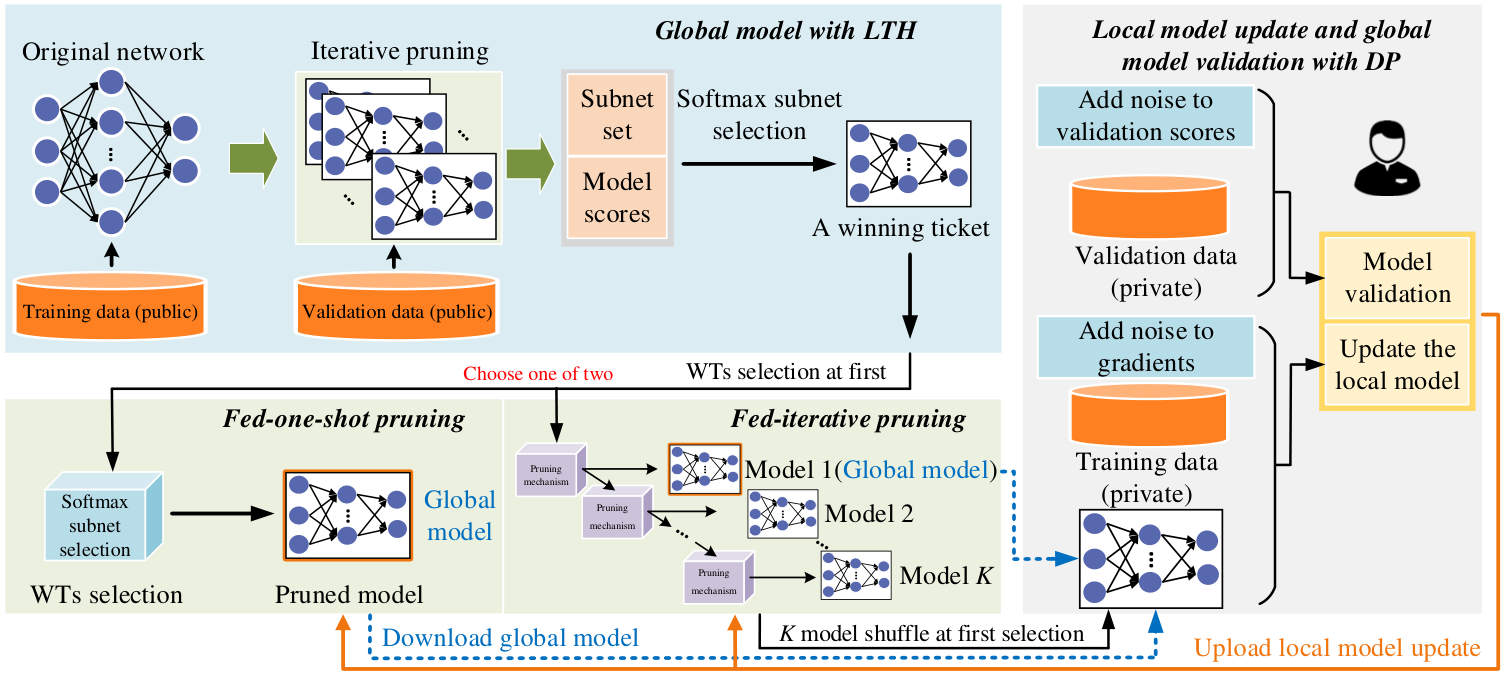
In this section, we give a detailed description of Fed-LTP. The overall framework is summarized in Algorithm 2, and its workflow from a client perspective is illustrated in Fig. 1.
IV-A Global Model Generation with LTH
Inspired by DPLTM [34], we use LTH to generate a candidate global model, which contains two major procedures (Algorithm 1).
1) WTs generation on public dataset with LTH. This process is identical to LTH, with the only difference being that we use the public dataset for WTs generation.
To find a lighter-weight network with higher test accuracy, an iterative pruning method is used when generating WTs. During the -th pruning, with the pruning degree to , a mask vector is set to zero if model is pruned or one if unpruned. Let denote the weight in the -th layer of model . Note that for the -th layer, the operation is defined as:
| (9) |
where and denotes the largest value of . Therefore, the mask matrix for model is constructed by applying (9) to each layer.
2) WTs selection with softmax function. Unlike the selection method in DPLTM [34], for the winning ticket selection, there are alternative tickets, and each ticket is given a score that equals to the correct number of samples for inference. To adjust the trade-off between the accuracy and the degree of network pruning, we use the softmax function [38] over the preference value also known as the score to select WT, which ensures that all WTs are explored:
| (10) |
where denotes one of possibly many winning tickets and is its corresponding probability. It is worth noting that we use LTH to generate WTs on the public dataset, and each client performs the training process with DP on their private data. Different from DPLTM [34], our method does not have the privacy budget as we do not use the private data while generating the model structure.
for to -1 do 1
Train the network for iterations on to obtain for -th winning ticket.
Prune of the parameters in , creating a mask by (9).
Reset the remaining parameters to their values in , generating the winning ticket and a pruned model . end for 2
Select a winning ticket with probability by (10) with the score.
Initialize model process: Firstly, select an initially pruned models by Global model generation with LTH (Algorithm 1). Secondly, get the models by Server-side model pruning.
for to do 1
Give the models by Client model selection to selected MTs.
for each selected client in parallel do 2
end for 4
for s=0 to do 5
where . end for 6
Return
Server-side model pruning:
if fed-iterative pruning then 7
end if 10
if fed-iterative pruning then 13
Model shuffle at first selection for client , and the
models of different MTs satisfy (14). end if 14
IV-B Server-side WT-broadcasting Mechanism
We propose a server-side WT-broadcasting mechanism with two major steps (Algorithm 2). It constrains the local and global models within the same model class to stabilize global model aggregation.
1) Server-side model pruning. We present two different pruning strategies for model pruning as below, and the final retention rate is denoted as .
Fed-one-shot pruning. Following the convention of LTH [27] and [39], let denote a selected client. According to Algorithm 1, weight-based pruning is conducted when generating WTs, and the WT selected by the softmax function can be used as the global model:
| (11) |
which results in .
Fed-iterative pruning. To achieve a better balance among test accuracy, communication cost, and resource overhead of edge devices than fed-one-shot pruning, fed-iterative pruning further prunes the global model based on LTH. Then we generate models with different pruning degrees following HeteroFL [31], where local models have similar architecture but can shrink their model size within the same global model class.

As shown in Figure 2, is decided by two pruning factors: (i). the initially selected WT’s retention rate ; (ii). the further pruning degree . In the further pruning stage, we repeatedly apply the weight-based pruning method in (9) to generate heterogeneous models by iterative pruning while the number of iterations is the same as the number of MTs selected each time. Formally, the model parameter of model at the -th training round is given by:
| (12) |
where denotes the element-wise product. Finally, the global model is produced by:
| (13) |
where for global training round . Note that the aggregated parameters are averaged over the unpruned parameters in each participated client, and the model structure is consistent with the client model with the highest retention rate.
2) Client model selection. In the fed-one-shot pruning strategy, only one global model is broadcast to all MTs, whereas in the fed-iterative pruning scheme, local model is obtained by model shuffle (without replacement) at first selection for client . It should be noted that in the subsequent training epoch, the MTs who have been selected do not participate in the model shuffle, and the models of other MTs selected at first are different from those of MTs who have been selected, that is:
| (14) |
To show the more details between the final retention rate and different client models by (12) in the fed-iterative pruning, the adaptive discount factor and of client are given by:
| (15) |
where and also represents the degree of variation across local models. Due to the different pruning degrees across MTs, is set to the average value of :
| (16) |
IV-C Local Model Training with DP
After the participated MTs download the initially pruned model from the server side, and then the MTs start the local model training with DP protection on their own private data. Due to the initial model having been pruned in the server-side WT-broadcasting mechanism, at -th communication round, each participated client performs local model iteration updates, at -th local iteration step, a mini-batch stochastic gradient is calculated on a mini-batch private data. And then we clip and add DP random noise into it, where the noise is satisfied by the Gaussian distribution . Thus, the local iteration is performed as:
After finishing the local iteration steps, we calculate the local model update:
Finally, each participated client sends the local model update to the server. The more details are also summarized in lines 13-19 of Algorithm 2. Note that the local model training process in private data also means performing knowledge transfer due to the local model being trained in the public data from the server side. Below, we present some discussion about the knowledge transfer between public and private data.
Knowledge transfer between public and private data. Since the use of public data is common in DP literature [40, 41, 39, 42], following the convention of [9, 39, 42], we utilize the labeled public data and the computational power of the server instead of the limited resources of the edge devices. In practice, we generate several pre-trained WTs on the public data, and then save the architecture of selected WT as the global model and reinitialize the values of unpruned parameters. Note that, unlike DPLTM [34], Fed-LTP does not require an additional privacy budget.
IV-D Model Validation with Laplace Mechanism
After all local model updates of the participated MTs are uploaded to the server, to select the best global model and prevent over-fitting, the server calculates the validation score based on the local validation datasets after the local model update with DP in each communication round. However, traditional schemes usually tune the hyperparameters using grid-search [18], which violates the rule of the real system due to observing the testing privacy data. Thus, testing private data is necessary to be protected for data privacy in the real system, thereby also consuming the privacy budget. In this paper, the Laplace mechanism is adopted to achieve the DP guarantee during the validation process.
At the beginning of each communication round, the server obtains a global model by aggregation. Then, it sends this global model to all MTs. Each client subsequently validates the received model based on its local validation dataset to obtain scores and sends it to the server. To protect the privacy of local validation dataset, each client needs to perturb the validation scores by:
| (17) |
where is the DP sensitivity and is the parameter for the Laplace distribution. It is clear that the maximum change of the score caused by a single sample is bounded as . The server obtains the validation scores for the global model as:
| (18) |
after receiving all MTs’ scores. Finally, when the FL training is terminated, the server selects the model with the highest validation score as the global model, that is:
| (19) |
From (18), as the number of participants in each round gets larger, the system can obtain a more reliable validation score as the variance of the aggregated noise is smaller.
V Privacy Analysis
In this section, we provide a tight privacy analysis based on zCDP for calculating the privacy loss/budget as communication round increases.
As shown in Figure 1 and Algorithm 2, the privacy budget with a given can be divided into two parts: local model training with DP and the DP-based model validation.
Theorem 1.
The accumulated privacy loss of the proposed algorithm after the -th communication round can be expressed as
| (20) |
where
| (21) |
In (21), denotes a Gaussian probability density function (PDF), is the PDF of a mixture of two Gaussian distributions, and is the sample rate of local gradient (mini-batch) in local model training.
Proof.
According to references [36] and [43], the privacy loss can be given by:
| (22) |
where is the Rényi -divergence, and is caused by the local model training with DP and the DP-based model validation, respectively. Specifically, based on [35] and [36], we can calculate as (21), where we use the Rényi distance to estimate the privacy loss. We denote by the random mechanism used in model validation. According to Lemma 1 for the validation process, if satisfies -DP, it also satisfies -zCDP. Consequently, it holds that:
| (23) |
Then, via considering (t+1) communication rounds, we can obtain
| (24) |
Based on (22) and (23), the privacy loss is accumulated as (20). ∎
During the training process, the cumulative privacy loss is updated at each epoch, and once the cumulative privacy loss exceeds the fixed privacy budget , the training process is terminated. To achieve an expected training time with a given total privacy budget, we can determine the values of hyperparameters for these schedules before training. Note that, for the validation-based schedule, the additional privacy cost needs to be taken into account due to the access to the validation dataset.
VI EXPERIMENTAL EVALUATION
The goal of this section is to evaluate the performance of Fed-LTP with different final retention rates on popular benchmark datasets and compare it with other baseline methods to demonstrate the superiority of our framework.
VI-A Experimental Setup
Baselines. To evaluate the performance of Fed-LTP, we compare it with several baseline methods: 1) DP-Fed: this baseline adds instance-level DP to Fed-Avg [2]; 2) Fed-SPA [18]: this baseline integrates random sparsification with gradient perturbation, and uses acceleration technique to improve the convergence speed.
Datasets and Data Partition. We evaluate Fed-LTP on four datasets: MNIST [44], FEMNIST [45], CIFAR-10 [46], and Fashion-MNIST [47], where FEMNIST and CIFAR-10 are regarded as the public data. Two experimental groups are presented with different private data: Fashion-MNIST and MNIST. Note that the implementation details and results on the Fashion-MNIST private data are presented in this paper. Meanwhile, detailed experimental evaluation on the MNIST private data is presented in the Appendix -D. We consider two different settings for all algorithms: both identical data distributed (IID) and non-identical data distributed (non-IID) settings across federated clients, such as MTs, where non-IID means the heterogeneous data distribution of local MTs. It can make the training of the global model more difficult. We partition the training data according to a Dirichlet distribution Dir() for each client [48] and generate the corresponding validation and test data for each client following the same distribution where is a concentration parameter controlling the uniformity among MTs. For the non-IID setting, we set , where MTs may possess samples of different numbers and classes chosen at random.
Implementation Details. The number of MTs is , and the server randomly selects a set of MTs with a sampling ratio of the MTs to participate in the training for all experiments. We set the privacy failure probability and the number of local iterations , with a fixed clipping threshold and a noise multiplier for all experiments. For the local optimizer on MTs, we use the momentum SGD and set the local momentum coefficient to , while set the learning rate as with a decay rate for FL process. Meanwhile, the learning rate for generating the WTs is set to be . is set to in the fed-iterative pruning scheme for all experiments. For the Fashion-MNIST private data, a CNN model is adopted and the number of communication rounds and Batch size . More implementation details are presented in Appendix -B. In addition, the privacy loss of all algorithms is calculated using the API provided in [43]. And the communication cost of the baseline methods is calculated in the same way as in Fed-SPA [18]. Each client in Fed-LTP also uses bits, where is the number of unpruned model parameters to be updated to the server.

VI-B Experimental Results
We run each experiment 3 times and report the test accuracy based on the validation datasets and the cumulative sum of upload and downstream communication costs across all rounds in each experiment. In the following, we focus on the evaluation of Fed-LTP from various aspects.
| Methods | Public data | (Average) | (Across selected MTs) | ||||
| Fed-LTP | FEMNIST | 0.20 | 0.44 | 0.27 | 0.16 | 0.10 | 0.06 |
| 0.29 | 0.52 | 0.36 | 0.25 | 0.18 | 0.12 | ||
| 0.40 | 0.59 | 0.47 | 0.38 | 0.30 | 0.24 | ||
| 0.54 | 0.66 | 0.60 | 0.54 | 0.48 | 0.44 | ||
| CIFAR-10 | 0.28 | 0.60 | 0.36 | 0.22 | 0.13 | 0.08 | |
| 0.39 | 0.70 | 0.49 | 0.34 | 0.24 | 0.17 | ||
| 0.53 | 0.79 | 0.64 | 0.51 | 0.41 | 0.33 | ||
| 0.73 | 0.89 | 0.80 | 0.72 | 0.65 | 0.59 | ||
| Fed-SPA | – | All | 1.00 | 1.00 | 1.00 | 1.00 | 1.00 |
| DP-Fed | – | 1.00 | 1.00 | 1.00 | 1.00 | 1.00 | 1.00 |
1) Efficient computation and memory footprint on MTs. Suppose that the model parameter is represented by a 32-bit floating number and the model compression ratio stored on MTs is , which is also regarded as the key parameter that can determine the size of computation overhead and memory footprint on MTs. Since the computational and memory footprint overhead required by MTs is proportional to the size of the training models, the resource constraint for MTs is alleviated when the model size is reduced. In particular, the local model is trained with the sparse-to-sparse technique in Fed-LTP, while the baseline methods Fed-SPA and DP-Fed use the dense-to-sparse and dense-to-dense training, respectively. In practice, Fed-SPA only reduces the uploading communication cost without reducing the model size, while DP-Fed trains the network without any model compression or pruning. Therefore, for all baselines, and for Fed-LTP. Furthermore, considering the resource heterogeneity across MTs, we propose the fed-iterative pruning strategy, where the values of among the selected MTs are different and small compared with baselines as shown in Table II, while for the fed-one-shot pruning strategy, the values of are the same as the value of . Consequently, the resource overhead of fed-iterative pruning is less than that of fed-one-shot pruning when choosing the same WT as the candidate global model.
2) Better utility-privacy trade-off. We compare the best testing accuracy of all algorithms under the same privacy budget, named the utility-privacy trade-off. In Fig. 3, Fed-LTP achieves better utility-privacy trade-off with two different pruning strategies than baselines on two datasets: FEMNIST and CIFAR-10 in both IID and non-IID settings. Specifically, with the same privacy loss, Fed-LTP has better test accuracy than baselines. For instance, when in Fig. 3(a), Fed-LTP increases the test accuracy by around and compared with baselines on FEMNIST in the IID and non-IID settings, respectively. Meanwhile, the convergence speed of the model training in Fed-LTP is higher than that in baselines. Therefore, Fed-LTP achieves a better utility-privacy trade-off, which means better model performance and stricter privacy guarantees.
3) Efficient communication. For each algorithm with its optimal retention rate, Fig. 4 shows its testing accuracy with respect to the cumulative sum of upload and downstream communication costs. On FEMNIST and CIFAR-10, the algorithm settings are: Fed-LTP (fed-iterative pruning, and , respectively; fed-one shot pruning, and , respectively), Fed-SPA (), and DP-Fed (). It is clear that for different settings and datasets, the cumulative total communication cost of Fed-LTP is lower than those of the baseline methods while having better convergence speed and test accuracy. As shown in Fig. 4(a) and Fig. 4(b), with the same communication cost, Fed-LTP under two pruning strategies always achieve better accuracy than baselines due to the use of LTH and further pruning the global model on the server side. Consequently, it is clear that Fed-LTP with two different pruning strategies are more communication-efficient than baselines, and the fed-one-shot pruning strategy is more communication-efficient than the fed-iterative pruning strategy. For instance, to achieve a target accuracy on FEMNIST in Fig. 4(a), in the IID setting, these two pruning strategies produce the communication cost of around MB and MB, respectively; in the non-IID setting, they yield the communication cost of around MB and MB.
This observation confirms that client heterogeneity and downstream cost are two meaningful factors affecting the model performance and communication efficiency, respectively.
VI-C Discussion of the Pruning Schemes and Retention Rates
In this section, the impact of pruning in Fed-LTP is investigated with various retention rates and pruning schemes for IID and non-IID data from FEMNIST.
Impact of pruning (the final retention rate ). In Fig. 5, as the retention rate decreases, the test accuracy tends to decrease. This can be analyzed from the perspective of parameter sharing, as the loss of model information perceived by the server is evident when the retention rate is small, causing significant errors in the training process. For instance, in Fig. 5(a), as the retention rate is set to , , , and with the fed-iterative pruning strategy in the IID setting, test accuracy decreases to around , , and , respectively. Furthermore, the decrease in test accuracy is particularly evident with the fed-iterative pruning than with the fed-one-shot pruning (e.g., and in both IID and Non-IID settings, respectively).
Impact of the pruning scheme. The difference in performance between fed-iterative pruning and fed-one-shot pruning strategies can be observed from Fig. 3 and Fig. 5, which is clear that the fed-iterative pruning achieves a performance similar to fed-one-shot pruning while reducing the resource overhead of MTs and communication cost. That means a better balance between performance, computation overhead, and communication cost can be achieved by reducing the complexity of the local models. However, especially in the non-IID setting as shown in Fig. 5(a), the performance is worse than fed-one-shot pruning due to the dual effects of both model and data heterogeneity as the (averaged) final retention rate decreases. Our current experimental study on the effect of data heterogeneity, and the effect of client heterogeneity across MTs is an interesting extension for future work.
VI-D Ablation Study
In this section, we present the ablation study of Fed-LTP. The purpose is to investigate the specific role and effect of a certain component or hyper-parameter in Fed-LTP, by fixing others to their default values. Ablation experiments are conducted on FEMNIST.
Effect of global model generation with LTH. LTH is used to generate a unified sparse structure of the global model while ensuring better model performance on the server side. To validate the effect of global model generation with LTH, we conduct experiments on Fed-LTP with two pruning strategies, and Fed-LTP without the global model generation for comparison, where the unpruned network is used. As in the case of LTH in a centralized learning scenario [27, 28, 29], Fig. 6 shows that the global model with the LTH module can improve the performance under the two pruning strategies: the test accuracies of Fed-LTP with fed-iterative pruning are improved by around and in the IID and non-IID settings, respectively. Therefore, with the fed-one-shot pruning, the performance gains are around and , respectively.

Effect of server-side WT-broadcasting mechanism. To verify the effect of the server-side WT-broadcasting mechanism, experiments are conducted on three schemes: 1) client-side WTs selection, where MTs generate and save WTs with local private data on the client side; 2) client-side transfer-WTs selection, where MTs only need to select and train a pretrained model created by the server side; 3) the server-side WT-broadcasting mechanism. The results in Fig. 8 show that the client-side WTs selection and client-side transfer-WTs selection schemes are inferior to the server-side WT-broadcasting mechanism with more volatile performance, due to the large variations in the structure of WTs generated by different MTs and the biased data distribution across MTs.
Effect of model validation with the Laplace mechanism. When the global model validation is not used on the server side, the global model in the final training process can be regarded as the final model. Therefore, the performance of the trained model usually deteriorates with a large number of rounds especially in the DP setting. This can result in a worse performance of the final model than using the global model validation. As shown in Fig 7, it is clear that the test accuracy of Fed-LTP with model validation is better in both settings and with different pruning schemes.
Effect of privacy loss computing method (zCDP). As the privacy analysis introduced in Section V, the privacy loss with zCDP can increase the level of privacy protection during the communication round. In Fig. 9, the results are generally worse in terms of both the convergence speed and the best accuracy of the global model than Fed-LTP without the privacy loss with zCDP. Therefore, zCDP is shown to be beneficial to the model utility and privacy guarantee in both settings and with different pruning schemes.
VII CONCLUSIONS
In this paper, we design a privacy-preserving algorithm in FL (Fed-LTP) that can properly balance computation, memory efficiency of edge devices, and communication efficiency with improved model utility. It contains a pre-trained model for exploring the sparse network structure and a differentially private global model validation mechanism to ensure the quality of the selected model against over-fitting. Meanwhile, we present the privacy analysis combining the privacy costs of model training and validation, and adopt the sparse-to-sparse training to save the limited resources of edge devices. Furthermore, the proposed noise-adding approach and the lightweight model can result in a better balance between the privacy budget and model performance. Finally, extensive experiments are conducted to verify the effectiveness and superiority of the proposed algorithm compared with SOTA methods. For future work, we will further investigate the effect of the iterative nature of the pruning method across clients/MTs with non-IID datasets. In addition, the ability to validate generalization guarantees on non-IID datasets also needs further exploration.
References
- [1] T. Li, A. K. Sahu, A. Talwalkar, and V. Smith, “Federated learning: Challenges, methods, and future directions,” IEEE Signal Processing Magazine, pp. 50–60, 2020.
- [2] B. McMahan, E. Moore, D. Ramage, S. Hampson, and B. A. y Arcas, “Communication-efficient learning of deep networks from decentralized data,” in Proc. International Conference on Artificial Intelligence and Statistics (AISTATS), vol. 54, April. 2017, pp. 1273–1282.
- [3] P. Kairouz, H. B. McMahan, B. Avent, A. Bellet, M. Bennis, A. N. Bhagoji, K. Bonawitz, Z. Charles, G. Cormode, R. Cummings et al., “Advances and open problems in federated learning,” Foundations and Trends® in Machine Learning, pp. 1–210, 2021.
- [4] F. Sattler, S. Wiedemann, K.-R. Müller, and W. Samek, “Robust and communication-efficient federated learning from non-iid data,” IEEE transactions on neural networks and learning systems, 2019.
- [5] J. Hamer, M. Mohri, and A. T. Suresh, “Fedboost: A communication-efficient algorithm for federated learning,” in International Conference on Machine Learning. PMLR, 2020.
- [6] R. Dai, L. Shen, F. He, X. Tian, and D. Tao, “Dispfl: Towards communication-efficient personalized federated learning via decentralized sparse training,” arXiv preprint arXiv:2206.00187, 2022.
- [7] Z. Xu, Z. Yang, J. Xiong, J. Yang, and X. Chen, “Elfish: Resource-aware federated learning on heterogeneous edge devices,” CoRR, 2019.
- [8] S. Wang, T. Tuor, T. Salonidis, K. K. Leung, C. Makaya, T. He, and K. Chan, “Adaptive federated learning in resource constrained edge computing systems,” IEEE Journal on Selected Areas in Communications, 2019.
- [9] Y. Jiang, S. Wang, V. Valls, B. J. Ko, W.-H. Lee, K. K. Leung, and L. Tassiulas, “Model pruning enables efficient federated learning on edge devices,” IEEE Transactions on Neural Networks and Learning Systems, Early Access 2022.
- [10] T. Huang, S. Liu, L. Shen, F. He, W. Lin, and D. Tao, “Achieving personalized federated learning with sparse local models,” arXiv preprint arXiv:2201.11380, 2022.
- [11] M. Fredrikson, S. Jha, and T. Ristenpart, “Model inversion attacks that exploit confidence information and basic countermeasures,” in Proc. ACM SIGSAC Conference on Computer and Communications Security (CCS), 2015, pp. 1322–1333.
- [12] R. Shokri, M. Stronati, C. Song, and V. Shmatikov, “Membership inference attacks against machine learning models,” in Proc. IEEE Symposium on Security and Privacy (SP), 2017, pp. 3–18.
- [13] L. Melis, C. Song, E. De Cristofaro, and V. Shmatikov, “Exploiting unintended feature leakage in collaborative learning,” in Proc. IEEE Symposium on Security and Privacy (SP), 2019, pp. 691–706.
- [14] M. Nasr, R. Shokri, and A. Houmansadr, “Comprehensive privacy analysis of deep learning: Passive and active white-box inference attacks against centralized and federated learning,” in Proc. IEEE Symposium on Security and Privacy (SP), 2019, pp. 739–753.
- [15] L. Zhang, L. Shen, L. Ding, D. Tao, and L.-Y. Duan, “Fine-tuning global model via data-free knowledge distillation for non-iid federated learning,” in Proceedings of the IEEE/CVF Conference on Computer Vision and Pattern Recognition, 2022, pp. 10 174–10 183.
- [16] C. Dwork and A. Roth, “The algorithmic foundations of differential privacy,” Found. Trends Theor. Comput. Sci., pp. 211–407, Aug. 2014.
- [17] N. Agarwal, A. T. Suresh, F. X. Yu, S. Kumar, and B. McMahan, “cpSGD: Communication-efficient and differentially-private distributed SGD,” in Proc. Annual Conference on Neural Information Processing Systems (NeurIPS), Dec. 2018, pp. 7575–7586.
- [18] R. Hu, Y. Gong, and Y. Guo, “Federated learning with sparsification-amplified privacy and adaptive optimization,” in Proc. Thirtieth International Joint Conference on Artificial Intelligence (IJCAI), Aug. 2021, pp. 1463–1469.
- [19] L. Sun and L. Lyu, “Federated model distillation with noise-free differential privacy,” in Proc. Thirtieth International Joint Conference on Artificial Intelligence (IJCAI), Aug. 2021, pp. 1563–1570.
- [20] L. Sun, J. Qian, and X. Chen, “LDP-FL: Practical private aggregation in federated learning with local differential privacy,” in Proc. Thirtieth International Joint Conference on Artificial Intelligence (IJCAI), Aug. 2021, pp. 1571–1578.
- [21] H. B. McMahan, D. Ramage, K. Talwar, and L. Zhang, “Learning differentially private recurrent language models,” in Proc. International Conference on Learning Representations (ICLR), Apr. 2018.
- [22] R. C. Geyer, T. Klein, and M. Nabi, “Differentially private federated learning: A client level perspective,” CoRR, Aug. 2017.
- [23] P. Kairouz, Z. Liu, and T. Steinke, “The distributed discrete gaussian mechanism for federated learning with secure aggregation,” in Proc. International Conference on Machine Learning (ICML), Jul. 2021, pp. 5201–5212.
- [24] R. Hu, Y. Gong, and Y. Guo, “Federated learning with sparsified model perturbation: Improving accuracy under client-level differential privacy,” CoRR, 2022.
- [25] A. Cheng, P. Wang, X. S. Zhang, and J. Cheng, “Differentially private federated learning with local regularization and sparsification,” CoRR, 2022.
- [26] Y. Shi, Y. Liu, K. Wei, L. Shen, X. Wang, and D. Tao, “Make landscape flatter in differentially private federated learning,” arXiv preprint arXiv:2303.11242, 2023.
- [27] J. Frankle and M. Carbin, “The lottery ticket hypothesis: Finding sparse, trainable neural networks,” in Proc. International Conference on Learning Representations (ICLR), 2019.
- [28] J. Frankle, G. K. Dziugaite, D. M. Roy, and M. Carbin, “Stabilizing the lottery ticket hypothesis,” arXiv preprint arXiv:1903.01611, 2019.
- [29] J. Frankle, G. K. Dziugaite, D. Roy, and M. Carbin, “Linear mode connectivity and the lottery ticket hypothesis,” in Proc. International Conference on Machine Learning (ICML), 2020, pp. 3259–3269.
- [30] A. Li, J. Sun, B. Wang, L. Duan, S. Li, Y. Chen, and H. Li, “LotteryFL: Personalized and communication-efficient federated learning with lottery ticket hypothesis on non-iid datasets,” in Proc. IEEE/ACM Symposium on Edge Computing (SEC), San Jose, CA, USA, Dec. 2021, pp. 68–79.
- [31] E. Diao, J. Ding, and V. Tarokh, “HeteroFL: Computation and communication efficient federated learning for heterogeneous clients,” arXiv preprint arXiv:2010.01264, 2020.
- [32] S. Itahara, T. Nishio, M. Morikura, and K. Yamamoto, “Lottery hypothesis based unsupervised pre-training for model compression in federated learning,” in Proc. IEEE Vehicular Technology Conference (VTC2020-Fall), 2020, pp. 1–5.
- [33] S. Seo, S.-W. Ko, J. Park, S.-L. Kim, and M. Bennis, “Communication-efficient and personalized federated lottery ticket learning,” in Proc. IEEE International Workshop on Signal Processing Advances in Wireless Communications (SPAWC), 2021, pp. 581–585.
- [34] L. Gondara, K. Wang, and R. S. Carvalho, “The differentially private lottery ticket mechanism,” arXiv preprint arXiv:2002.11613, 2020.
- [35] M. Abadi, A. Chu, I. J. Goodfellow, H. B. McMahan, I. Mironov, K. Talwar, and L. Zhang, “Deep learning with differential privacy,” CoRR, 2016.
- [36] I. Mironov, “Rényi differential privacy,” in Proc. IEEE computer security foundations symposium (CSF), 2017, pp. 263–275.
- [37] M. Bun and T. Steinke, “Concentrated differential privacy: Simplifications, extensions, and lower bounds,” in Proc. International Conference Theory of Cryptography (TCC), ser. Lecture Notes in Computer Science, vol. 9985, Beijing, China, Oct.-Nov. 2016, pp. 635–658.
- [38] E. Jang, S. Gu, and B. Poole, “Categorical reparameterization with gumbel-softmax,” arXiv preprint arXiv:1611.01144, 2016.
- [39] Z. Luo, D. J. Wu, E. Adeli, and L. Fei-Fei, “Scalable differential privacy with sparse network finetuning,” in Proc. IEEE/CVF Conference on Computer Vision and Pattern Recognition (CVPR), 2021, pp. 5057–5066.
- [40] J. Wang and Z.-H. Zhou, “Differentially private learning with small public data,” in Proc. AAAI Conference on Artificial Intelligence (AAAI), 2020.
- [41] N. Papernot, S. Song, I. Mironov, A. Raghunathan, K. Talwar, and Ú. Erlingsson, “Scalable private learning with pate,” arXiv preprint arXiv:1802.08908, 2018.
- [42] T. Li, M. Zaheer, S. Reddi, and V. Smith, “Private adaptive optimization with side information,” in International Conference on Machine Learning. PMLR, 2022, pp. 13 086–13 105.
- [43] A. Yousefpour, I. Shilov, A. Sablayrolles, D. Testuggine, K. Prasad, M. Malek, J. Nguyen, S. Gosh, A. Bharadwaj, J. Zhao, G. Cormode, and I. Mironov, “Opacus: User-friendly differential privacy library in pytorch,” CoRR, 2021.
- [44] Y. LeCun, L. Bottou, Y. Bengio, and P. Haffner, “Gradient-based learning applied to document recognition,” Proceedings of the IEEE, vol. 86, no. 11, pp. 2278–2324, 1998.
- [45] S. Caldas, S. M. K. Duddu, P. Wu, T. Li, J. Konečnỳ, H. B. McMahan, V. Smith, and A. Talwalkar, “Leaf: A benchmark for federated settings,” arXiv preprint arXiv:1812.01097, 2018.
- [46] A. Krizhevsky, G. Hinton et al., “Learning multiple layers of features from tiny images,” 2009.
- [47] H. Xiao, K. Rasul, and R. Vollgraf, “Fashion-mnist: a novel image dataset for benchmarking machine learning algorithms,” arXiv preprint arXiv:1708.07747, 2017.
- [48] T.-M. H. Hsu, H. Qi, and M. Brown, “Measuring the effects of non-identical data distribution for federated visual classification,” arXiv preprint arXiv:1909.06335, 2019.
-A Notation and high parameters
In Table I, we present the notion and high parameters used in this paper.
-B Implementation details
Models. For the MNIST private dataset, the CNN model consists of two 5 5 convolution layers with the ReLu activation function (the first with 10 filters, the second with 20 filters, each followed with 2 2 max pooling), a fully connected layer with 320 units and the ReLu activation function, and a final softmax output layer, referred to as model 1. For the Fashion-MNIST private dataset, a CNN model is adopted, which is identical to model 1 except that the convolutional layer size is 3 3 with the ReLu activation function (the first with 32 filters, the second with 64 filters) and a fully connected layer has 512 units, referred to as model 2. In addition, the number of communication rounds and Batch size for model 1, and and for model 2.
Datasets. There are 60K training examples and 10K testing examples on the datasets: MNIST, FEMNIST, and Fashion-MNIST. Specifically, The MNIST and Fashion-MNIST datasets consist of 10 classes of 28 28 handwritten digit images and grayscale images, respectively. The FEMNIST dataset is built by partitioning the data in Extended MNIST based on the writer of the digit/character, which consists of 62 classes. The CIFAR-10 dataset consists of 10 classes of 32 32 images. There are 50K training examples and 10K testing examples in the dataset.
-C The detail of experimental results on the Fashion-MNIST private data
| Methods (The final retention rate: ) | FEMNIST | CIFAR10 | |||||||
| Acc | Comm(MB) | Acc | Comm(MB) | ||||||
| IID | Non-IID | IID | Non-IID | ||||||
| Fed-LTP (fed-iterative pruning) | 72.25 | 71.23 | 31.66 | 5.35 | 75.16 | 72.57 | 34.38 | 5.35 | |
| Fed-LTP (fed-one-shot pruning) | 73.65 | 70.86 | 35.30 | 5.35 | 75.87 |
|
38.34 | 5.35 | |
| Fed-SPA, = 1 | 74.40 | 68.40 | 64.36 | 9.71 | 74.40 | 68.40 | 64.36 | 9.71 | |
| Fed-SPA, = 0.8 | 72.21 | 69.09 | 57.92 | 8.78 | 72.21 | 69.09 | 57.92 | 8.78 | |
| Fed-SPA, = 0.6 | 70.45 | 65.40 | 51.49 | 7.77 | 70.45 | 65.40 | 51.49 | 7.77 | |
| Fed-SPA, = 0.4 | 69.21 | 69.23 | 45.05 | 6.60 | 69.21 | 69.23 | 45.05 | 6.60 | |
| Fed-SPA, = 0.2 | 65.26 | 68.96 | 38.62 | 5.16 | 65.26 | 68.96 | 38.62 | 5.16 | |
| DP-Fed | 70.41 | 68.89 | 64.36 | 9.71 | 70.41 | 68.89 | 64.36 | 9.71 | |
We compare the best testing accuracy of all algorithms under the same privacy budget, named the utility-privacy trade-off, which is shown in Figure 3. Furthermore, we list the final results in Table III, which summarizes the final results of DP-Fed, Fed-SPA, and Fed-LTP after rounds on Fashion-MNIST private dataset in both IID and non-IID settings. The cost of the baseline methods is calculated in the same way as in Fed-SPA [18]. Each client in Fed-LTP uses bits, where is the number of unpruned model parameters to be updated to the server.
It is very clear that there are three main evaluation indicators and that our algorithm achieves a good balance between them. In order to facilitate discussion and comparative analysis, the following sections are divided into separate discussions and analyses of other indicators under a fixed indicator. We can see that the performance in the non-IID setting is generally worse than that in the IID setting due to the data heterogeneity across the federated clients. Moremore, Fed-LTP under the two pruning strategies also achieves a better trade-off between accuracy and communication cost, in comparison to the two baseline methods DP-Fed and Fed-SPA with different final retention rates . Specifically, Fed-SPA features better test accuracy but also higher communication and privacy costs when is large. Meanwhile, DP-Fed is generally worse than Fed-LTP in terms of test accuracy and communication cost.
-D The detail of experimental results on the MNIST private data
The results are the same as that on Fashion-MNIST private dataset. In particular, we list the evaluation from various aspects.
-D1 Efficient computation and memory footprint of edge devices.
The computational and memory footprint overhead required by edge devices is proportional to the size of the training models. On the MNIST private dataset, the training model size is the same as the model size on the Fashion-MNIST private dataset. Therefore, the results of computation and memory footprint overheads are also the same as the results on the Fashion-MNIST private dataset as shown in Table II.
-D2 Better utility-privacy trade-off.
In Figure 10, we present the best testing accuracy of all algorithms under the same privacy budget . It is clearly seen that Fed-LTP generates better testing accuracy under a smaller privacy budget. That means our algorithm achieves a better utility-privacy trade-off, which is same as the results on Fashion-MNIST private dataset.
-D3 Efficient communication.
In Figure 11, we present the best testing accuracy of all algorithms under the same communication cost. It is clearly seen that Fed-LTP generates better testing accuracy at a smaller cost. That means our algorithm achieves a better utility-communication trade-off, which is same as the results on Fashion-MNIST private dataset.
