Keywords: Positive streamer discharge, axial streamer model, model reduction.
Submitted to Plasma Sources Sci. Technol.state of August 11, 2026
Estimating the properties of single positive air streamers from measurable parameters
Abstract
We develop an axial model for single steadily propagating positive streamers in air. It uses observable parameters to estimate quantities that are difficult to measure. More specifically, for given velocity, radius, length and applied background field, our model approximates the ionization density, the maximal electric field, the channel electric field, and the width of the charge layer. These parameters determine the primary excitations of molecules and the internal currents. Our approach is to first analytically approximate electron dynamics and electric fields in different regions of a uniformly-translating streamer head, then we match the solutions on the boundaries of the different regions to model the streamer as a whole, and we use conservation laws to determine unknown quantities. We find good agreement with numerical simulations for a range of streamer lengths and background electric fields, even if they do not propagate in a steady manner. Therefore quantities that are difficult to access experimentally can be estimated from more easily measurable quantities and our approximations. The theoretical approximations also form a stepping stone towards efficient axial multi-streamer models.
1 Introduction
1.1 The challenge of model reduction
Streamer discharges occur widely in nature and technology [1]. The most commonly encountered and studied streamers appear in air and carry positive net charge at their heads. They are the topic of the present study.
The inner structure of a streamer consists of a thin moving curved space charge layer around a weakly ionized channel with strong field enhancement and steep electron density gradients at the tip. This is challenging to simulate numerically, even for a single axisymmetric streamer in a long gap and a low background electric field [2]. On the other hand many discharge phenomena consist of numerous interacting streamers [1, 3, 4, 5, 6]. This poses a strong motivation to reduce the model while not giving up the physical basis and the model validation achieved in recent years [2, 7, 8, 9].
Streamer discharges consist of clearly distinguishable regions where different physical mechanisms are dominating the behaviour: (i) a non-ionized outer area where the electrostatic Poisson equation has to be solved, (ii) the avalanche zone where photoionization creates many growing electron avalanches, (iii) the moving streamer heads with an active space charge layer where ionization increases rapidly and the field is highest, and (iv) ionized channels with charges and currents and dynamically changing conductivity. Since the regions are governed by different mechanisms we will analyse them separately. Later we match the different regions at their boundaries.
For the channel region an axial approximation has been formulated in [10, 11], but for the streamer head the problem is open. In this work we will concentrate on the heads. To allow for comparison between numerical simulations of the fluid model and analytical approximations, we constrain the analysis to single streamers in a uniform field and mostly to steady propagation.
1.2 Steady streamers as a test case
In sufficiently low electric fields a streamer can propagate at a constant velocity without changing shape [12, 13, 14, 15]. Such streamers leave no charge behind and their channel electric fields decay back to the applied background field. From now on we will refer to these as steady, because in a co-moving coordinate system such uniformly translating streamers are in a steady state. The properties of positive steady streamers can be considered extreme, with velocities as low as m/s, electric fields enhanced to values as high as 222 kV/cm, steep gradients and a strongly curved thin charge layer [14].
The analysis presented in this work focuses heavily on steady streamers, since it is mathematically convenient to consider steady state solutions, as they have no explicit time dependence in a co-moving frame. Furthermore, we validate our approximations by comparing them to simulated results of a steady streamer. It must be noted that such a steady state approach could also be considered for accelerating streamers, since their properties typically change slowly with respect to other relevant time scales [16]. To that end we also compare our approximations to simulations of three accelerating streamers.
1.3 Earlier work
A classical challenge is to develop equations of motion where the head is characterized by a few numbers like radius and velocity . One of the first proposed analytic relations between and date back to 1965 [17] and an ‘order-of-magnitude’ model for the parameters of streamers was given in 1988 [18, 19]. A later experimental investigation proposed a data fit where the velocity depends on the radius squared, i.e. [20], and in [21] an approximate relation based on [17] was proposed where the velocity is also a function of the maximum electric field at the tip , i.e. . Other important theoretical results are: an approximation for the ionization density [19, 22, 23], energy efficiency estimates for radical production [24], an analytic investigation of the avalanche zone dynamics [25], 1.5D models that require a prescribed radius [16, 26] and an estimate for charge layer width based on the notion of an effective ionization length [27]. An application of streamer theory is to infer difficult-to-measure properties, such as , from measurable parameters. For example, in [28] the authors estimate a parameter range for on the basis of observed radius and velocity. Another example is [25], where an analysis of the avalanche zone gives an approximate relation between , and the head potential.
These theoretical results have improved our understanding of streamer dynamics and illustrated complex relations between different parameters. However, some ideas proposed in earlier works fail to agree with results from numerical simulations. At several instances throughout this work we will provide an in-depth evaluation of earlier work and propose improvements.
1.4 Content of the paper
In this work we develop semi-analytic approximations for the fluid model of single positive streamers that estimate difficult-to-measure quantities based on observable parameters. Specifically, we will show how velocity , radius of curvature , length and background field determine ionization density , charge layer width and the maximum and channel electric fields and , respectively:
| (1) |
The derivation of our model starts by first defining different regions where specific physical mechanisms dominate. Then we provide analytic approximations for each of these regions separately. Finally we match the different regions at their boundaries and implement a self-consistent solution method. This results in a self-contained axial model which agrees well with numerical simulations. This means that our framework can complement experimental measurements when important streamer characteristics, i.e. the parameters on the right-hand side of equation (1), are difficult to measure precisely.
In section 2 we outline the classical fluid streamer model and the numerical implementation used for axisymmetric simulations. Furthermore, we discuss the results of numerical simulations in detail and introduce important definitions and conventions. In section 3 we integrate through the charge layer and obtain an analytic formula for the ionization density. In section 4 we give an analysis of the electron avalanche dynamics in the region ahead of the streamer. In section 5 we explore the notion of the streamer head potential. In section 6 we describe our solution method and validate our approximations with numerical results of the fluid model.
2 Model description, definitions and conventions
In this section we will present the classical fluid model for positive streamers in air at standard temperature and pressure. We discuss the numerical implementation, used to obtain reference solutions in homogeneous background electric fields below the breakdown value. The same implementation was used in [12, 13] to study steady streamers. Furthermore, we will also give definitions of macroscopic parameters and clarify other conventions and terminology.
2.1 Description of the model
2.1.1 Basic equations.
We employ the classic fluid streamer model with local field approximation and without ion mobility. We only account for two charged species: the electron density and the net ion density , with denoting the number density of all positive or negative ions. One can use just one ion density instead of several ion species in regions where ion drift, electron detachment, and electron ion recombination can be neglected, as is the case in the streamer head. The electron density evolves according to a drift-diffusion-reaction equation while ions are considered immobile
| (2) | ||||
| (3) |
with the electric field, the electron mobility, and the electron diffusion coefficient. and are the source terms for the effective impact ionization and photo-ionization respectively. We neglect electron diffusion, which is typically a good approximation except in low where we have steep gradients in the charge layer. Effective impact ionization is given by
| (4) |
where is the drift current density of electrons, is the electric current density, is the elementary charge, and is the effective ionization coefficient. The data for the transport and reaction coefficients are discussed in the next section. The photo-ionization source term in a volume is given by
| (5) |
with the source of ionizing photons, the absorption function and is a geometric factor. Following Zheleznyak’s model [29, 30], can be expressed as
| (6) |
with the actual pressure, mbar the quenching pressure of the gas-mixture, and a proportionality factor relating impact excitation to impact ionization . The absorption function is given by
| (7) |
with (mm bar), (mm bar), and is the partial pressure of oxygen. For air at 300 K and 1 bar, the corresponding absorption lengths are 33 m and 1.9 mm.
The electric field follows from Poisson’s equation for the electric potential
| (8) | ||||
| (9) |
with the dielectric constant, the elementary charge, and the charge number density.
2.1.2 Implementation of axisymmetric simulations.
In this work we compare our axial analytical approximations with the axisymmetric solutions of equations (3)-(9) obtained by numerical simulation. The numerical model uses the afivo-streamer code [31, 32]. The computational setup is the same as in earlier studies [12, 13] to which we refer for an in-depth discussion.
The transport and reaction coefficients are calculated by Bolsig+ [33] (version 12/2019) using cross sections from the Phelps database [34] under the assumption that the evolution of the electron density follows an exponential temporal growth or decay [35]. We use the same data for the analytical and the numerical models. Additionally, the numerical model for the axisymmetric simulations uses continuity equations for a number of species such as O, O, N, N, etc. as listed in [13]. This more extended plasma chemistry model helps stabilizing the steady streamer at the lowest background electric field, and it is consistent with the two-species model for and in the streamer head, as recalled above.
The photo-ionization integral in equation (5) is approximated by a set of Helmholtz differential equations with Bourdon’s three-term approximation [36]. This approximation introduces small changes the photon absorption lengths. However, in [35, 37] it was shown this has essentially no measurable influence on streamer discharge propagation in air.
Computational domain.
The computational domain consists of a cylinder with 40 mm length and 20 mm radius, and planar electrodes on top and below. We impose cylindrical symmetry for domain and streamers; and we call the longitudinal coordinate , and the radial coordinate . An electric field is applied in the -direction by fixing an electric potential difference between the electrodes. We use homogeneous Neumann boundary conditions for the potential in the -direction, which means that the electric field is parallel to the lateral boundary. Homogeneous Neumann boundary conditions are also used for the electron density on all boundaries.
Initial conditions.
For the initiation of a streamer discharge, we placed two neutral seeds composed of electrons and positive ions at the upper boundary of the domain. The uppermost seed creates a region of field enhancement, and the seed below it supplies the initial electrons ahead of the forming streamer, before photo-ionization sets in. More details on the seeds — their densities, coordinates, and sizes — can be found in [12, 13].
In low electric fields, an initial transient electric field is needed to ensure the inception of a streamer discharge. In this research we will consider homogeneous background electric fields from 4.5 to 24 kV/cm, all below the breakdown value of 28 kV/cm. At 4.5 kV/cm, a streamer propagating at constant velocity and shape was obtained using the velocity control method [14]. At 10 kV/cm we adopt the same initial transient electric field as discussed in [13].
To accommodate for the relatively small size of the steady streamer we used a grid with a minimum cell width of 0.6 m. For the accelerating streamers, the mesh refinement routines are identical to those in [13].

2.2 Description of axisymmetric simulation results
2.2.1 The steady streamer in detail.
In this section we will discuss one of these simulations in detail, the steady streamer at a background electric field of 4.5 kV/cm. We recall that a steady streamer [13, 12, 14, 15] looses its conductivity at its back end due to electron attachment and electron ion recombination, that it leaves no electric charge behind, but carries a fixed amount of charge along, and that it propagates with constant velocity and shape. Figure 1 zooms into the front part of this streamer and shows four important quantities: the electron density , the magnitude of the electric field, the magnitude of the electric current density and the charge number density . From these quantities we can distinguish three regions with different dynamics:
- 1.
The channel is the conductive interior of the streamer. We have a high electron density here and the plasma is quasi-neutral, . The electron density in the low axial electric field gives rise to an electric current flowing along the channel.
- 2.
The charge layer is a layer of (positive) charge which surrounds and partially screens the channel. At the streamer head, the curvature of the charge layer leads to high electric field enhancement ahead of the front. In fact, we find the maximum electric field here, with its location denoted by . As the electron density is high as well, we here have a high impact ionization rate and large currents resulting in the movement of the streamer head. The charge layer in the streamer head is also referred to as the ionization front. The width of the charge layer is much smaller than its radius of curvature; this is required for the strong field enhancement ahead of the layer.
- 3.
The avalanche zone of a positive streamer is the region ahead of the charge layer, so the electric charges in this region have a negligible effect on the electric field distribution. Without photo-ionization or some background electron density it could be neglected, but for positive streamers in air the photo-ionization creates many growing electron avalanches moving towards the charge layer. Close to the layer there is a high electric field, which means that a significant electron current is created which maintains the active ionization front. Specifically in air without background ionization, the electron density vanishes with an asymptotic decay dictated by photon absorption [38]
(10)
2.2.2 Directions of currents and fields.
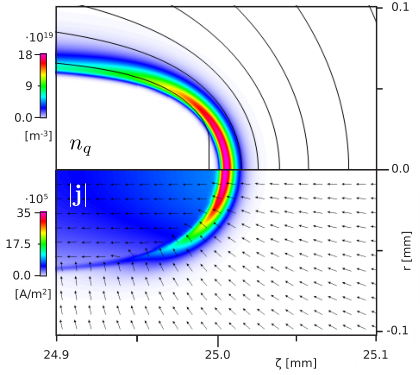
In figure 2 we zoom further into the ionization front and highlight important geometric features. We show the charge number density and the magnitude of the electric current density again in color-coding, but additionally we have visualized the direction of the current density by normalized arrows in the lower half of the plot, and the equipotential lines in the upper half of the plot. Note that in the avalanche zone the direction of the electron current is radially inwards in a nearly spherical geometry, whereas in the channel the electron drift is homogeneously directed backwards parallel to the axis of propagation. Furthermore, the equipotential lines are very well aligned with the charge layer. This means that the electric current is essentially perpendicular to the layer in this region.
2.2.3 Streamers in different fields.
In figure 3 we show current densities, electric fields and electron and charge densities on the streamer axis, now not only for the steady streamer in the field of 4.5 kV/cm, but also for accelerating streamers in background fields of 14 and 24 kV/cm when the streamer heads reached mm. In more detail, the upper plots show the electric current density. The middle plots show the electric field (solid line) with our approximation (dashed line) of section 3.2, and the lower plots show , and .
2.3 Definitions and conventions
In this paper we develop an axial model for the dynamics in charge layer and avalanche zone, based on analytical approximations. Here we introduce definitions and conventions for this purpose. A schematic is given in figure 4.
2.3.1 Definition of velocity and co-moving coordinate system.
We define the streamer velocity as the velocity of the location of the maximal electric field at the streamer tip
| (11) |
The velocity extracted from simulations is shown in figure 5(a). We introduce a coordinate system that moves in the direction with velocity . The coordinate can be written as
| (12) |
Temporal derivatives transform to the new coordinate system as
| (13) |
where denotes the partial derivative in the co-moving frame . For steady motion we thus can replace
| (14) |
in the co-moving frame .
2.3.2 Parameterizing the charge layer.
We will characterize the charge layer by two maxima, namely the maximum of the electric field and the maximum of the charge number density. On the streamer axis we will denote them as and , and their distance as
| (15) |
in the co-moving coordinate system defined below. The two maxima are also illustrated in figure 3. There it is also shown that is located roughly in the middle of the charge layer and that is approximately symmetric in the vicinity of this maximum. Therefore we define the interior boundary of the charge layer as
| (16) |
2.3.3 Definition of radius and of origin of coordinate system.
We will characterize the streamer head by its radius of curvature , defined as the radius of the circle which best approximates the curved charge layer at the streamer tip. This parameter is extracted from simulated data by fitting a semicircle through the maximum, for each , of the charge layer, cf. figure 4. The extracted is insensitive to fitting parameters provided the region is chosen sufficiently small. We therefore take this region to be . The radius of curvature extracted from simulations is shown in figure 5(b).
is an important quantity because it determines the spatial decay of electric field and currents in the avalanche zone near the charge layer, as can be seen in figure 2. There the equipotential lines trace the shape of the charge layer sufficiently close to the axis of propagation. We choose the centre of the sphere as the origin of the co-moving coordinate system, , as shown in Fig. 4.
2.3.4 Definition of streamer length for steady streamers
The steady positive streamers reported in [12, 13, 14] are all ‘detached’ from their point of inception. By this we mean that due to attachment and recombination processes the channel looses its conductivity to the point that the streamer cannot be considered as connected to an electrode or initial ionized seed. For these detached streamers it is more useful to characterize streamer length with a typical length scale for the loss of conductivity
| (17) |
with the electron loss time representing the collective timescale of all conductivity loss processes. The studies [13, 14] contain investigations of and . In particular, it is analyzed how these quantities depend on the gas-composition and the electric field.
3 The charge layer
In this section we formulate axial approximations for the total current density and for the electron and ion densities in the space charge layer, i.e., in the region between the front end of the channel and the maximum of the electric field (cf figure 4). The width of this region is much smaller than the radius of curvature , therefore this layer can approximately be treated as planar.
We can neglect photo-ionization in the charge layer since it is much smaller than . Photo-ionization only matters in the avalanche zone due to its nonlocality. We also neglect the diffusive current assuming that it is dominated by convection.
3.1 Current densities in the charge layer
Due to charge conservation and the Poisson equation of electrostatics, the total current density is a conserved quantity
| (18) |
For steady motion in a co-moving frame , the total current is . Note that the current densities are taken in the stationary frame, expressed as a function of .
To solve for we approximate the charge layer at the tip as a planar surface. The validity of this approximation is governed by the dimensionless parameter . More specifically we require , which usually holds for streamers as is shown in figure 6. In that case only the -derivative of the divergence operator is non-vanishing. Then, equation (18) prescribes that is constant. With a boundary condition at this leads to the axial approximation
| (19) |
Furthermore, the electric field is maximal at , hence and the displacement current vanishes there
| (20) |
where is the electron current density on axis at . Similarly, the displacement current also vanishes approximately in the channel, where the electric field and electron density are nearly constant on-axis. This gives us
| (21) |
where is defined analogously as . Finally, combining this result with equation (19) determines .
An analysis of the total current density at and was also proposed in [39]. They held that vanishes which would mean that is completely determined by the displacement current . However, the numerical simulations in figure 3 contradict this. In fact, we observe that at the displacement current vanishes since the electric field is maximal and conversely that does not vanish, which is in line with our reasoning.
3.2 Ionization and electric field in the charge layer
As ions are essentially immobile within the propagating streamer head, the degree of ionization is best determined by the ion density behind the charge layer. An old approximation dating back to [19, 22] is
| (22) |
where we use . In the appendix of [23] this equation is derived for planar negative streamer ionization fronts without electron diffusion or photo-ionization. The approximation is easily derived from the two following equations: equations (3) and (4) together yield
| (23) |
and equation (18) reads , if the total current ahead of the charge layer vanishes. This is the case, if the electron density ahead of the planar front vanishes, and if the electric field ahead of the front does not change in time.
According to [23], equation (22) is a good approximation of the numerical solutions of planar negative ionization fronts without photo-ionization in a time independent electric field; the error is only 5 to 10%. However, in simulations of positive curved streamer fronts with photo-ionization as shown in [40, 14], the ionization density is about twice as high as given by the classical approximation (22) (in particular, see table B1 of [14]). In table 1 we make a similar comparison and confirm the discrepancy of equation (22) as an approximation of the ionization density of positive streamers.
| classical | new | ||
|---|---|---|---|
| eq. (22) | eq. (26) | simulation | |
| 4.5 kV/cm | 11.9 | 21.9 | 25.6 |
| 10 kV/cm | 3.3 | 5.4 | 6.3 |
| 14 kV/cm | 3.4 | 5.6 | 6.3 |
| 24 kV/cm | 4.5 | 7.6 | 8.4 |
A first hypothesis was that the approximation (22) only covers the part of the front where the electric field decays from its maximal value to a low value inside the channel, and that it misses the avalanche zone ahead of the charge layer where the electric field increases to its maximum [40]. This avalanche zone is essentially absent without background ionization and photo-ionization, but very present in air. However, the ionization created in the avalanche zone contributes relatively little ionization. We discuss this later in more detail in section 6.2 and figure 8.
We will now show that the total current density from the avalanche zone into the curved charge layer contributes significantly to the ionization behind the front for positive streamers in air. The derivation of the new approximation is analogous to the earlier one in [23]. We start from (23) and express in terms of
| (24) |
This can be further simplified due for steady motion and because the vectors and are parallel on the axis
| (25) |
Integration through the ionization front gives
| (26) | ||||
The first term is obtained after integration by substitution . It reproduces the old approximation (22) when it is evaluated at and when is approximated as vanishing. The second term requires further analysis. We approximate by the constant according to equation (19). Furthermore, we need the spatial profile of to evaluate under the integral. Here we adopt a heuristic parametrization of and leave further analysis to future work. In figure 3 we see that within the layer the charge number densities have an approximately Gaussian profile that can be parameterized as
| (27) |
with
| (28) |
an approximate normalization constant provided that .
Next, we use that over its small width the layer is only weakly curved, and we use a planar approximation to calculate the electric field as by integrating over
| (29) |
This heuristic parametrization of the electric field is shown in the middle panels of figure 3 together with the results of the axisymmetric simulations. The parametrizations of are in agreement with the simulated results when we choose for the steady streamer and for the accelerating ones. Furthermore, we remark explicitly that equation (27) is only used to motivate and evaluate the parameterization for in equation (29).
Using equation (29) as an approximation for the electric field within the charge layer, we can calculate the ionization density by evaluating equation (26) at . In table 1 we compare this approximation, when all macroscopic parameters are extracted from simulations. We observe good agreement, with relative errors between 10-15%.
3.3 Electron density in the charge layer
Our derivation of the electron density within the charge layer starts from the fundamental equation of charge conservation
| (30) |
Since we have uniform translation and a planar front we can write
| (31) |
where has been introduced as an integration constant. As a side note, a similar relation has also been proposed in [22, 28], but there the integration constant has been explicitly neglected. However, in figure 3 we see that and are significant. Continuing our derivation, we use and rearrange the terms in this equation such that we find an expression for the electron density profile in the charge layer
| (32) |
with the charge drift velocity . (Note that electrons drift with ). This determines since is given by equation (26). By evaluating this expression at or and using equation (21) we find quasi-neutrality: and . Note that the implied quasi-neutrality at only holds as an approximation, see figure 3.
Moreover, integration of equation (31) through the charge layer and using (28) results in
| (33) |
This can be interpreted as a physical connection between the movement of a positive charge layer (represented by a discontinuity in the electric field) and the separation of charge. The latter can be directly expressed by the electric current integrated through the charge layer.
4 The avalanche zone ()
The avalanche zone is defined as the region ahead of the space charge layer where space charges can be neglected, and where the electric field is above the breakdown value. This means that the electric field near this layer is dominated by the electric charges in the layer, and that charges in the avalanche zone move in this externally determined field, but do not contribute to it.
In the avalanche zone, different approximations have to be made than in the charge layer:
- (i)
As said above, the influence of the local charges on the electric field is negligible, , so the avalanche develops in an externally determined electric field.
- (ii)
The dynamics inside the charge layer were described using the planar front approximation because , but the planar front approximation is not valid in the avalanche zone. We therefore do account for the curvature of the charge layer in the avalanche zone. We do so by approximating the charge layer at the streamer tip as a hemisphere with a radius , see figures 4 and 7.
- (iii)
Electron diffusion is still neglected but photoionization now needs to be included. Although the impact ionization is much stronger than the photoionization, the non-locality of the photoionization is essential to create seed electrons in the avalanche zone.
4.1 Equation for electron density in the avalanche zone
The drift-diffusion-reaction equation (2) for the electron dynamics on the axis of the avalanche zone can be simplified as follows. First we remark that with the approximations above and with the chain-rule we can write on the axis
| (34) | ||||
The electron dynamics of equation (2) then becomes, in the comoving frame on the axis,
| (35) |
In the next section we derive an expression for .
4.2 Coupling between avalanche zone and charge layer
The dynamics in the avalanche zone are coupled to the other discharge regions. More precisely, the charge layer together with the channel generate the enhanced electric field in the avalanche zone, and the charge layer also emits the large majority of photons that generate photoionization and initiate the ionization avalanches in the avalanche zone.
The electric field near the charge layer and near the streamer axis are approximated by a uniformly charged sphere
| (36) |
as argued above.
For photoionization in air, the photons are mainly produced in the charge layer, because the majority of high-energy collisions occurs here, as will be shown in figure 8. Photons originating from the avalanche zone are therefore neglected. Moreover, since typical absorption lengths (331900 m for dry air at 1 bar and 300 K) are large compared to , cf figure 9, we can essentially treat the charge layer as a surface. Accordingly, we approximate equation (5) by a surface integral
| (37) |
with the unit vector in the -direction, and the coordinates now lie on the surface . For simplicity, we take to be the surface of a hemisphere with radius centered at . This is illustrated in figure 7.
The general photon source term from equation (6) is now approximated as
| (38) |
with the surface density of photon production
| (39) |
on the streamer axis. Here is the quenching factor of the photon emitting state. The excitation of the photon emitting state is approximated as impact ionization times a proportionality factor . Note that the impact ionization has to be integrated over the width of the charge layer which is obtained after integrating (from equation (3)) across the charge layer. Finally, since we have omitted the dependency on .
is a function that can account for the fact that the impact ionization and thus the photon radiation in the charge layer diminishes in the off-axis direction. However, for simplicity we take . Naturally this will slightly overestimate photon radiation.
4.3 Solving the electron density in the avalanche zone
We will now solve equation (35). To do so we first introduce the short hand notation
| (40) |
with the electron avalanche growth function
| (41) |
and the photoelectron source term
| (42) |
in the external electric field from equation (36). is determined by equations (37) – (39) as a surface-integral corresponding to the parametrized charge layer. For given , equation (40) is an ordinary differential equation for that is solved as
| (43) |
This solution can be interpreted as a superposition of electron avalanches. The electron avalanches are continuously created by a photoelectron density . The avalanches grow in the electric field as described by which contains the effects of impact ionization and of electron mobility .
For further evaluation, it is interesting to discuss the structure of this solution and the implications for the electron and ion densities at the front and back end of the charge layer, and . We find that equation (43) can be rewritten as
| (44) |
with an explicit equation for the function that does not depend on any electron or ion densities. Here , and determine the electric field in the avalanche zone according to (36). That does not depend on the particle densities, is due to the linear nature of the avalanche zone without local space charge effects: twice as many photons emitted from the charge layer will create twice as many avalanches and twice as many electrons arriving at which in turn emit twice as many photons from the charge layer.
The explicit equation for the function is
| (45) |
where the first line contains the field dependent electron dynamics on the streamer axis, and the second line the field independent photon dynamics between the charge layer and the axis.
An analysis of the avalanche zone along similar lines was proposed in [25], but they only account for photons produced in the avalanche zone and neglect the contribution from the charge layer. However figure 3 shows that ionization in the charge layer, and therefore the associated photon production, is far more important. In our approach we do take the charge layer as the dominant photon source. The same reasoning was also given in [26, 16]. In addition to this we have derived an improved photoionization balance on the basis of consistent electrodynamics in the charge layer and avalanche zone, equation (44). This formula replaces the photoionization balance proposed in [25]. We finally remark that the balance between the dynamics of photons and of electron avalanches resembles a self-sustained DC discharge, with the difference that the anode is replaced by a propagating streamer head with self-consistent shape.
5 The electrostatic field and the head potential
5.1 Streamer head potential
As recalled in [1], the electrostatic approximation for the electric field is sufficient for streamer physics. Therefore the line integral between any two points is independent of the path taken between them
| (46) |
with any continuous curve which starts at and ends at . This concept will be applied to derive a relation between the electrostatic properties of the channel and the head.
We shall use equation (46) to solve two path-integrals, the first corresponding only to the background field and the second to the field with a streamer present. In both cases equals the axis of propagation, i.e. -axis, which gives and on the opposing electrode. For the streamers in this work is far away from the opposing electrode, which means that boundary effects are negligible and we can take at infinity. When we subtract the two integrals we find
| (47) |
since the potential at and is the same and therefore the right-hand side vanishes. This fundamental property has been considered by previous authors [41, 25, 15, 14, 42]. Equation (47) will be split in two intervals with different dynamics, namely: the streamer channel and the avalanche zone . We shall treat each of these intervals separately.
5.1.1 Potential across the channel.
The potential across the channel requires different treatment for steady and accelerating streamers.
For a steady streamer the channel electric field decays back to the background field. In general the profile of the channel electric field is determined by currents in the streamer channel [10, 11]. For now, modelling the charge distribution within the channel is not considered. Instead, we suggest a plausible channel electric field profile for steady streamers. In section 2.3 we have discussed how dynamics in the channel are related to an electron loss time scale , which in turn defines an electron loss length . We use these concepts to impose
| (48) |
Substituting this into equation (47) results in
| (49) |
For the accelerating streamers considered in this work we have , which means it is more reasonable to work with an averaged channel electric field . By holding that over the length of the channel we can obtain a similar result
| (50) |
5.1.2 Potential across the avalanche zone.
In the avalanche zone the electric field was approximated by that of a uniformly charged sphere, equation (36). Using this the potential across the avalanche zone simplifies approximately to
| (51) |
This gives the final result
| (52) |
To keep notation simple we have no longer discerned between or for the separate cases of steady and accelerating streamers.
6 Solving the approximations
6.1 Solution method
We now assume that velocity , radius of curvature , length and background electric field are given, for example by experimental measurements, and we estimate four unknowns that are much more difficult to measure: ionization density , maximal electric field , channel field , and charge layer width . To that end we shall formulate a system of four relations from which these unknowns will be determined.
In the previous sections we have derived equations (21) and (33) by analyzing the dynamics of the charge layer , where . These are the first and second relations. On the basis of electrostatics we have related the head potential to the streamer length in equation (52), which is the third relation. Finally, we require that charge layer and avalanche zone electron dynamics are consistent (cf. section 4.3). This introduces the last relation, namely equation (44). For convenience, we repeat our relations here
| (53) | ||||
| (54) | ||||
| (55) | ||||
| (56) |
The function is defined in equation (4.3) and the electron current density is defined as . The above system of equations has independent parameters:
| (57) |
All other quantities are determined by these parameters. To see this, we summarize our approximations in the two regions:
- •
In the avalanche zone the electric field and the electron density are approximated by (equations (36) and (43))
(58) (59) Notably, the function (equation (42)) accounts for the production of photoelectrons and is proportional to . The electron density and the electric field by definition give and therefore . Finally, we have assumed that space charge effects are negligible in the entire avalanche zone. We therefore also assume quasi-neutrality at the tip .
- •
In the charge layer the electric field and densities are approximated by (equations (29), (26), (32))
(60) (61) (62) where in equation (60) is a parametrization given in equation (27). The quantities and are determined by the avalanche zone. Quasi-neutrality in the channel gives . Thus we can evaluate and within the charge layer.
The objective is then to determine parameters in (57), since we consider that are fixed by observations. The remaining four, which we call , have to satisfy our relations (53)-(56). Solving this system of equations is equivalent to finding the roots of the four-dimensional vector-function , which is defined as the difference between the left- and right-hand sides of equations (53)-(56). Thus is a consistent solution if it satisfies
| (63) |
Due to the complexity of we employ an iterative root-finding algorithm that solves equation (63) using a modification of the Levenberg-Marquardt algorithm [43]. Such an algorithm starts from an initial guess and produces a sequence of values that converges to the root. We emphasize again that the input parameters , , and in addition to are sufficient to evaluate . Moreover, changing the initial guess seems to have no effect on the obtained solution , suggesting that the solution is unique. We observe the same in numerical simulations [14, 15].
6.2 Results
6.2.1 Steady streamer:
In this section we will compare the approximated , , , and with numerical simulations. We shall first do this comparison for the steady streamer. To obtain these results we extracted kV/cm, mm/ns, m and mm from simulation (see figure (5)) and used these to solve equation (63).
In figure 8 we show our approximation for the axial electron density of the steady streamer (equations (32) and (43)). The approximated electron density was overlaid onto the results from the numerical simulation such that the respective overlap. We observe that our analytic formulae for the electron density profile in the avalanche zone reproduces the profile obtained from simulation well. In this figure we can also observe that more than of the ionization occurs in the charge layer. This underlines our earlier arguments that ionization predominantly occurs in the charge layer and that photons originating from the avalanche zone can be neglected.
The approximated parameters , , and that were derived in this evaluation are shown in figure 9. We observe good agreement with a maximum relative error of about for the prediction of . The other parameters agree within .
6.2.2 Accelerating streamers:
As discussed in the introduction, we shall now apply our analysis developed for steady streamers to accelerating streamers. We include results, calculated in the same manner, for streamers at background electric fields of , and kV/cm. The corresponding velocity and radius as a function of streamer length were already shown in figure 5.
The approximated parameters are included in figure 9. In this case we also observe good agreement with relative errors of at most several tens of percent. Only at kV/cm do we have relative errors of about for the estimation of . Furthermore, we also illustrate the error introduced by our simplified treatment of the channel electric fields. For accelerating streamers we have included both and the averaged in figure 9. In section 5 we have used in order to obtain an equation for the channel electric fields without resolving the entire charge transport dynamics of the channel. However, this approximation is generally not true and the accuracy is worst for the kV/cm case. This has various causes, such as a persisting neutral seed (i.e. due to shorter propagation times the influence of initial conditions still persist), actual inhomogeneities in the channel or the influence of boundary conditions.
Overall, our model is also able to estimate the properties of streamers in higher background fields. Evidently, approximating the charge layers of accelerating streamer heads as planar fronts in a steady state gives reasonable results.
7 Summary and outlook
7.1 Summary
In this work we have proposed a model that characterizes a single positive air streamer on the basis of observable parameters. Overall, our approximations exhibit good agreement with numerical simulations of a steady streamer with typical relative errors below . For accelerating streamers the errors are slightly higher, with a maximum deviation up to % in the highest considered background field.
Our most important theoretical contributions are:
- •
We have constructed a self-contained axial model that can approximate macroscopic properties of steady streamer heads. This model also gives good results for accelerating streamer heads.
- •
We have shown how the quantities , , and can be determined from the more easily observable parameters , , and .
- •
We have provided a formula for the ionization density of a streamer. Notably this formula contains the contribution due to a non-zero total current density and is about twice as high as the classical formula.
- •
We have given a self-consistent description of electron dynamics which includes the implicit contribution due to photoelectrons produced in the avalanche zone.
7.2 Outlook
For future work we recommend three possible improvements:
- •
We have not considered explicitly solving the dynamics of the charge layer. Instead we have accounted for these dynamics by heuristic parameterizations. However, a numerical approach that resolves densities and the electric field inside the charge layer can be expected to improve the accuracy. Moreover such an approach could replace a number of parameterizations, which would lead to a more precise representation of streamer dynamics.
- •
We have used two approaches for the channel electric fields. For accelerating streamers we have used an average value , and for steady streamers we have used an exponential decay with a prescribed length scale . These clearly have their limitations. In future work we aim to combine the insights obtained in this research with models that explicitly evaluate the dynamics of the streamer channel, such as [11].
- •
All derivations in this work assume that the dynamics of the charge layer can be approximated in a planar front setting, since the dimensionless parameter is typically small. A systematic expansion in terms of will likely improve the accuracy of our model.
Finally we comment on the significance of our work regarding the development of accurate streamer tree models such as [10, 11]. The current limitation of these models is that they lack a self-consistent description of velocity and radius of a streamer. These parameters are often imposed. However, our model can be combined with a tree model in order to overcome this critical limitation for positive streamers.
Acknowledgements
HF was funded by the European Union’s Horizon 2020 Research and Innovation Programme under the Marie Skłodowska-Curie Grant Agreement SAINT722337.
References
References
- [1] Nijdam S, Teunissen J and Ebert U 2020 Plasma Sources Science and Technology 29 103001 ISSN 1361-6595 URL https://iopscience.iop.org/article/10.1088/1361-6595/abaa05
- [2] Bagheri B, Teunissen J, Ebert U, Becker M M, Chen S, Ducasse O, Eichwald O, Loffhagen D, Luque A, Mihailova D, Plewa J M, van Dijk J and Yousfi M 2018 Plasma Sources Science and Technology 27 095002 ISSN 1361-6595 URL https://iopscience.iop.org/article/10.1088/1361-6595/aad768
- [3] Cummer S A, Jaugey N, Li J, Lyons W A, Nelson T E and Gerken E A 2006 Geophysical Research Letters 33 ISSN 00948276
- [4] Kochkin P O, Nguyen C V, Van Deursen A P and Ebert U 2012 Journal of Physics D: Applied Physics 45 ISSN 00223727
- [5] Hare B M, Scholten O, Dwyer J, Ebert U, Nijdam S, Bonardi A, Buitink S, Corstanje A, Falcke H, Huege T, Hörandel J R, Krampah G K, Mitra P, Mulrey K, Neijzen B, Nelles A, Pandya H, Rachen J P, Rossetto L, Trinh T N, Ter Veen S and Winchen T 2020 Physical Review Letters 124 ISSN 10797114
- [6] Sterpka C, Dwyer J, Liu N, Hare B M, Scholten O, Buitink S, Veen S t and Nelles A 2021 Geophysical Research Letters 48 2520–2533 ISSN 0094-8276 URL https://onlinelibrary.wiley.com/doi/10.1029/2021GL095511
- [7] Li X, Dijcks S, Nijdam S, Sun A, Ebert U and Teunissen J 2021 Plasma Sources Science and Technology 30 095002 ISSN 0963-0252 URL https://iopscience.iop.org/article/10.1088/1361-6595/ac1b36
- [8] Dijcks S, der Leegte M v and Nijdam S 2023 Plasma Sources Science and Technology 32 ISSN 13616595
- [9] Wang Z, Dijcks S, Guo Y, van der Leegte M, Sun A, Ebert U, Nijdam S and Teunissen J 2022 arXiv preprint arXiv:2208.07279
- [10] Luque A and Ebert U 2014 New Journal of Physics 16 013039 ISSN 1367-2630 URL https://iopscience.iop.org/article/10.1088/1367-2630/16/1/013039
- [11] Luque A, González M and Gordillo-Vázquez F J 2017 Plasma Sources Science and Technology 26 125006 ISSN 1361-6595 URL https://iopscience.iop.org/article/10.1088/1361-6595/aa987a
- [12] Francisco H, Bagheri B and Ebert U 2021 Plasma Sources Science and Technology 30 025006 ISSN 0963-0252 URL https://iopscience.iop.org/article/10.1088/1361-6595/abdaa3
- [13] Francisco H, Teunissen J, Bagheri B and Ebert U 2021 Plasma Sources Science and Technology 30 115007 ISSN 0963-0252 URL http://arxiv.org/abs/2107.06781https://iopscience.iop.org/article/10.1088/1361-6595/ac2f76
- [14] Li X, Guo B, Sun A, Ebert U and Teunissen J 2022 Plasma Sources Science and Technology 31 065011 ISSN 0963-0252 URL http://arxiv.org/abs/2201.11257https://iopscience.iop.org/article/10.1088/1361-6595/ac7747
- [15] Guo B, Li X, Ebert U and Teunissen J 2022 URL http://arxiv.org/abs/2204.02698http://dx.doi.org/10.1088/1361-6595/ac8e2e
- [16] Pavan C, Martinez-Sanchez M and Guerra-Garcia C 2020 Plasma Sources Science and Technology 29 095004 ISSN 0963-0252 URL https://iopscience.iop.org/article/10.1088/1361-6595/aba863
- [17] Loeb L B 1965 Ionizing Waves of Potential Gradient Tech. Rep. 3676
- [18] Dyakonov M and Kachorovskii V 1988 Sov. Phys. JETP 67 1049–1054
- [19] D’yakonov M and Kachorovskii V 1989 Zh. Eksp. Teor. Fiz 95 1850–1859 URL http://www.jetp.ac.ru/cgi-bin/dn/e_068_05_1070.pdf
- [20] Briels T M P, Kos J, Winands G J J, van Veldhuizen E M and Ebert U 2008 Journal of Physics D: Applied Physics 41 234004 ISSN 0022-3727 URL https://iopscience.iop.org/article/10.1088/0022-3727/41/23/234004
- [21] Naidis G V 2009 Physical Review E - Statistical, Nonlinear, and Soft Matter Physics 79 3–6 ISSN 15393755
- [22] Naidis G V 1997 Journal of Physics D: Applied Physics 30 1214–1218 ISSN 00223727
- [23] Li C, Brok W J, Ebert U and Van Der Mullen J J 2007 Journal of Applied Physics 101 1–17 ISSN 00218979
- [24] Naidis G V 2012 Plasma Sources Science and Technology 21 042001 ISSN 0963-0252 URL https://iopscience.iop.org/article/10.1088/0963-0252/21/4/042001
- [25] Pancheshnyi S, Starikovskaia S M and Starikovskiy A 2001 Journal of Physics D: Applied Physics 34 105–115 ISSN 0022-3727 URL https://iopscience.iop.org/article/10.1088/0022-3727/34/1/317
- [26] Lehtinen N 2021 Izvestiya vysshikh uchebnykh zavedenii. Radiofizika 64 12–28 ISSN 0021-3462 URL https://elibrary.ru/doi_resolution.asp?doi=10.52452%2F00213462_2021_64_01_12
- [27] Niknezhad M, Chanrion O, Holbøll J and Neubert T 2021 Plasma Sources Science and Technology 30 115014 ISSN 0963-0252 URL https://iopscience.iop.org/article/10.1088/1361-6595/ac3214
- [28] Babaeva N Y and Naidis G V 2021 Journal of Physics D: Applied Physics 54 223002 ISSN 0022-3727 URL https://iopscience.iop.org/article/10.1088/1361-6463/abe9e0
- [29] Zhelezniak M B, Mnatsakanian A K, Sizykh S V, Zhelezniak M B, Mnatsakanian A K and Sizykh S V 1982 HTemS 20 357–362 URL https://ui.adsabs.harvard.edu/abs/1982HTemS..20..357Z/abstract
- [30] Pancheshnyi S 2014 Plasma Sources Science and Technology 24 015023 ISSN 0963-0252 URL https://iopscience.iop.org/article/10.1088/0963-0252/24/1/015023
- [31] Teunissen J and Ebert U 2017 Journal of Physics D: Applied Physics 50 474001 ISSN 0022-3727 URL https://iopscience.iop.org/article/10.1088/1361-6463/aa8faf
- [32] Teunissen J and Ebert U 2018 Computer Physics Communications 233 156–166 ISSN 00104655 URL https://doi.org/10.1016/j.cpc.2018.06.018https://linkinghub.elsevier.com/retrieve/pii/S0010465518302261
- [33] Hagelaar G J and Pitchford L C 2005 Plasma Sources Science and Technology 14 722–733 ISSN 09630252
- [34] Phelps database, retrieved March 2019 URL www.lxcat.net
- [35] Wang Z, Sun A and Teunissen J 2022 Plasma Sources Science and Technology 31 ISSN 13616595
- [36] Bourdon A, Pasko V P, Liu N Y, Célestin S, Ségur P and Marode E 2007 Plasma Sources Science and Technology 16 656–678 ISSN 09630252
- [37] Bagheri B and Teunissen J 2019 Plasma Sources Science and Technology 28 045013 ISSN 1361-6595 URL https://iopscience.iop.org/article/10.1088/1361-6595/ab1331
- [38] Bouwman D, Teunissen J and Ebert U 2022 Plasma Sources Science and Technology 31 045023 ISSN 0963-0252 URL http://arxiv.org/abs/2203.00442https://iopscience.iop.org/article/10.1088/1361-6595/ac64bf
- [39] Babaeva N Y and Naidis G V 1997 IEEE Transactions on Plasma Science 25 375–379 ISSN 00933813
- [40] Luque A and Ebert U 2010 Geophysical Research Letters 37 n/a–n/a ISSN 00948276 URL http://doi.wiley.com/10.1029/2009GL041982
- [41] Kulikovsky A A 1998 Physical Review E 57 7066–7074 ISSN 1063-651X URL https://link.aps.org/doi/10.1103/PhysRevE.57.7066
- [42] Starikovskiy A, Bazelyan E and Aleksandrov N L 2022 Plasma Sources Science and Technology ISSN 0963-0252 URL https://iopscience.iop.org/article/10.1088/1361-6595/aca04c
- [43] Moré J J, Garbow B S and Hillstrom K E 1980 User guide for minpack-1 Tech. rep. CM-P00068642