[orcid=0000-0002-4447-0480]

Multi-directional Sobel operator kernel on GPUs

Qiong Chang Address: School of Computing, Tokyo Institute of Technology, Japan q.chang@c.titech.ac.jp Xiang Li Address: School of Electronic Science & Engineering, Nanjing University, China Yun Li yli@nju.edu.cn Jun Miyazaki

Abstract

Sobel is one of the most popular edge detection operators used in image processing. To date, most users utilize the two-directional $3\times{3}$ Sobel operator as detectors because of its low computational cost and reasonable performance. Simultaneously, many studies have been conducted on using large multi-directional Sobel operators to satisfy their needs considering the high stability, but at an expense of speed. This paper proposes a fast graphics processing unit (GPU) kernel for the four-directional 5x5 Sobel operator. To improve kernel performance, we implement the kernel based on warp-level primitives, which can significantly reduce the number of memory accesses. In addition, we introduce the prefetching mechanism and operator transformation into the kernel to significantly reduce the computational complexity and data transmission latency. Compared with the OpenCV-GPU library, our kernel shows high performances of 6.7x speedup on a Jetson AGX Xavier GPU and 13x on a GTX 1650Ti GPU.

keywords

Sobel operator ,multi-directional ,acceleration algorithm ,graphics processor

^†^†corresponding: Corresponding author

1 Introduction

The Sobel operator is a classical first-order edge detection operator that performs a 2D spatial gradient measurement on images and is generally used to find the approximate absolute gradient magnitude at each pixel. It is typically used to emphasize regions of high spatial frequency that correspond to edges. Compared with other edge detection operators, such as the Canny and Roberts cross, the Sobel operator has a low calculation amount, simple structure, and high precision. Therefore, it has a wide range of applications in fields such as remote sensing [1], medical image processing [2], and industrial detection [3].

To date, most applications using Sobel have chosen the two-directional $3\times{3}$ operator as their detectors because of its low computational cost and reasonable performance. Nevertheless, some applications still require further size expansions and increases in the direction of the operator to satisfy their unique requirements. In the medical field, Sheik et al. [4] proposed a Sobel operator for the edge detection of the knee-joint space of osteoarthritis. They improved the operator by adding $315^{\circ}$ and $360^{\circ}$ directions on the bias of horizontal and vertical directions, which can perform the detection better than the original two. Remya et al. [5] applied the Sobel operator to the edge detection of brain tumors in MRI images. Their operator was improved to handle eight directions to clearly detect extremely irregularly shapes of tumors and showed a higher detection accuracy than other methods. In the industrial field, Min et al. [6] utilized the Sobel operator to detect the edges of screw threads. Considering the type of screw thread angles are mainly $30^{\circ}$ , $55^{\circ}$ and $60^{\circ}$ , they assigned spatial weights and added $67.5^{\circ}$ and $112.5^{\circ}$ directions for the operator, which can efficiently extract more precise edges and achieve better continuity than conventional methods. In addition to the direction, Siyu et al. [7] expanded the operator size from $3\times{3}$ to $7\times{7}$ using the average gradient vectors of two neighboring pixels to quantify aggregate angularity. Compared with conventional methods using one pixel, the improved method helps calculate a more stable angularity index value. All these applications demonstrated that, in some cases, a large multi-directional Sobel operator has higher robustness than the traditional operator and can better adapt to actual requirements. However, as mentioned in [4], it always requires more computing time. In particular, as the image size increases, the amount of computation increases exponentially, which burdens applications using edge detection as a preprocessing step.

This paper proposes a fast graphic processing unit (GPU) kernel for a four-directional $5\times{5}$ Sobel operator, because GPUs usually show an excellent performance on real-time image processing problems [8] [9]. In our experience, a 5 $\times$ 5 Sobel operator has similar edge detection robustness to a 7 $\times$ 7 operator but higher than 3 $\times$ 3. Meanwhile, the processing speed of a multi-directional 5 $\times$ 5 operator is significantly slower than a 3 $\times$ 3 operator [10]. To improve kernel performance, we made innovations in the following aspects:

•

we implement the kernel based on warp-level primitives, which can significantly reduce the number of memory accesses;
•

we provide an efficient procedure with the prefetching mechanism, which significantly reduces the computational complexity and data transmission latency, and
•

we further accelerate the operations in diagonal directions using a two-step optimization approach, which helps to increase the data reuse rate.

The remainder of this paper is organized as follows. Section 2 introduces the acceleration strategies and results of the current Sobel operator. Section 3 provides the principle of the four-directional $5\times{5}$ Sobel operator. In Section 4, we introduce the implementation and optimization details of our GPU kernel. Then, we evaluate the kernel performance in Section 5 and finally conclude this paper in Section 6.

2 Related Work

Recently, several studies have been conducted on accelerating the Sobel edge detection using GPUs.

Jo et al. [11] optimized their GPU-based Sobel kernel using shared memory. They assigned the entire image to several blocks and used the corresponding streaming multiprocessors (SMs) to detect edges in parallel with their respective local information. This approach is simple and versatile but has limited performance improvement because the overuse of shared memory typically affects the number of active blocks and reduces the parallelism of the kernel. Nevertheless, the shared memory approach is 1.65x faster than that of global memory.

Chouchene et al. [12] realized a fast grayscale and Sobel edge detection on GPUs, which was approximately 50x faster than running on a CPU. Similar to [11], they split the edge detection task to each SM and stored the image fragments in the corresponding shared memory. The difference is that they enabled different sizes of CUDA blocks to accomplish the detection task, which proved more efficient in their application than the block-size consistent method.

Xiao et al. [13] proposed an eight-directional Sobel operator on GPU using the open computing language (OpenCL) framework. In their implementation, each work item handles the convolution calculations for four pixels instead of one, which can significantly improve memory access efficiency and reduce computational complexity. Compared with approaches implemented by CPU, OpenMP, and CUDA, they are 9.55, 2.23, and 1.17x faster, respectively.

Zuo. et al. [14] implemented a fast Sobel operator on GPUs. They optimized their GPU kernel as follows: 1) using the texture memory to store image data to accelerate memory access; 2) performing a single thread to process the calculations of multiple pixels, which can significantly increase the overall throughput and 3) fully exploiting the symmetry of Sobel operators to reuse intermediate results to reduce the entire computational complexity. They achieved a 122x acceleration ratio for a $4096\times{4096}$ image compared with the CPU-based implementation. However, owing to the limitation of texture memory size, it is unreasonable for common situations that require multiple images in practical applications.

The purposes of all the these methods are to accelerate the Sobel-based edge detection as fast as possible, while ensuring the correctness of results to satisfy real-time processing requirements. However, owing to the limitations of their parallel algorithms under GPU architectures, much room remains for improving their acceleration methods. Then, we will introduce an in-depth acceleration method for the Sobel operator.

Refer to caption — Figure 1: Edge detection results. (a) Original image. (b) Two-directional $3\times{3}$ . (c) Four-directional $3\times{3}$ . (d) Four-directional $5\times{5}$ .

3 Four-Directional $5\times{5}$ Sobel Operator

3.1 Operator Definition

The Sobel operator is a classical edge detection operator proposed by Irwin Sobel and Gary Feldman [15]. It is a discrete differential operator that detects the edge features of images by computing the pixel gradients. The original Sobel operator is an isotropic gradient operator using two $3\times{3}$ filters to convolve with an image and obtain derivative approximations: one each for horizontal and vertical changes. Equation 1 shows the basic computation of the Sobel operator:

G_{x}=\begin{bmatrix}-1&\textbf{0}&1\\ -2&\textbf{0}&2\\ -1&\textbf{0}&1\end{bmatrix}\ast{I}\\ ,G_{y}=\begin{bmatrix}-1&-2&-1\\ \textbf{0}&\textbf{0}&\textbf{0}\\ 1&2&1\end{bmatrix}\ast{I},

(1)

where $I$ represents the input image, and $G_{x}$ and $G_{y}$ are the two images containing the horizontal and vertical derivative approximations, respectively. $\ast$ denotes the basic convolution calculation between the input image and the two filters. In these two filters, because the weights of the central axis in both directions are $0$ , and the two sides in both directions are opposite to each other, the convolution results are equivalent to calculating the differences between the two sides, which means calculating the gradients in both directions. Then, the final result can be aggregated by calculating the root sum of square (RSS) of $G_{x}$ and $G_{y}$ as follows:

G=\sqrt{G_{x}^{2}+G_{y}^{2}}.

(2)

Figure 1(a) shows the original images, and Fig. 1(b) shows the local edge images (the yellow boxes in Fig. 1(a)) detected using the original two-directional $3\times{3}$ Sobel operator. Although some texture information is lost, the overall contour of the petals, houses, and figures are clearly preserved.

The original Sobel operator considers only the horizontal ( $0^{\circ}$ ) and vertical ( $90^{\circ}$ ) directions. To further enhance its effect, we introduce a $5\times{5}$ Sobel operator by adding two diagonal directions ( $45^{\circ}$ and $135^{\circ}$ ). The filters of the four-directional $5\times{5}$ Sobel operator can be defined as follows:

$\displaystyle G_{x}$	$\displaystyle=\begin{bmatrix}-1&-2&\textbf{0}&2&1\\ -4&-8&\textbf{0}&8&4\\ -6&-12&\textbf{0}&12&6\\ -4&-8&\textbf{0}&8&4\\ -1&-2&\textbf{0}&2&1\end{bmatrix}\ast{I},$	(3)
$\displaystyle G_{y}$	$\displaystyle=\begin{bmatrix}-1&-4&-6&-4&-1\\ -2&-8&-12&-8&-2\\ \textbf{0}&\textbf{0}&\textbf{0}&\textbf{0}&\textbf{0}\\ 2&8&12&8&2\\ 1&4&6&4&1\end{bmatrix}\ast{I},$
$\displaystyle G_{d}$	$\displaystyle=\begin{bmatrix}-6&-4&-1&-2&\textbf{0}\\ -4&-12&-8&\textbf{0}&2\\ -1&-8&\textbf{0}&8&1\\ -2&\textbf{0}&8&12&4\\ \textbf{0}&2&1&4&6\end{bmatrix}\ast{I},$
$\displaystyle G_{dt}$	$\displaystyle=\begin{bmatrix}\textbf{0}&-2&-1&-4&-6\\ 2&\textbf{0}&-8&-12&-4\\ 1&8&\textbf{0}&-8&-1\\ 4&12&8&\textbf{0}&-2\\ 6&4&1&2&\textbf{0}\end{bmatrix}\ast{I},$

and the final results can be aggregated as follows:

G=\sqrt{G_{x}^{2}+G_{y}^{2}+G_{d}^{2}+G_{dt}^{2}},

(4)

where $G_{d}$ and $G_{dt}$ represent the two images containing the diagonal derivative approximations. They can be obtained by rotating $G_{x}$ and $G_{y}$ by $45^{\circ}$ . In general, users can define the filter weights according to their needs and must only combine the Gaussian smoothing and differentiation. In Eq. 3, the weight values are generated using the OpenCV Sobel library and used to perform the edge detection shown in Fig. 1(d). To better distinguish the effect from the $3\times{3}$ operator, the detection results obtained by the four-directional $3\times{3}$ operator are listed in Fig. 1(c). Compared with the two-directional operator, the four-directional operator provides more abundant textures, such as petals and buildings. Furthermore, $5\times{5}$ operator is more insensitive to surrounding changes and less affected by noise, which helps provide clearer edge features and higher robustness than using $3\times{3}$ .

However, a four-directional $5\times{5}$ operator without optimization is approximately eight times more computationally intensive than the two-directional $3\times{3}$ , which significantly slows the processing speed. Therefore, developing an efficient acceleration method for the four-directional $5\times{5}$ operator is essential.

3.2 Filter Weight Generalization

To avoid limiting our method to the constant weight values in Eq. 3, we generalize our Sobel operator as follows:

$\displaystyle K_{x}$	$\displaystyle=a\cdot{\begin{bmatrix}1\\ n\\ m\\ n\\ 1\end{bmatrix}}\times{\begin{bmatrix}-1&-b&\textbf{0}&b&1\end{bmatrix}}$	(5)
	$\displaystyle=a\cdot{\begin{bmatrix}-1&-b&\textbf{0}&b&1\\ -n&-nb&\textbf{0}&nb&n\\ -m&-mb&\textbf{0}&mb&m\\ -n&-nb&\textbf{0}&nb&n\\ -1&-b&\textbf{0}&b&1\end{bmatrix}}=(k_{ij})_{5\times 5},$
$\displaystyle K_{y}$	$\displaystyle=a\cdot{\begin{bmatrix}-1\\ -b\\ \textbf{0}\\ b\\ 1\end{bmatrix}}\times{\begin{bmatrix}1&n&m&n&1\end{bmatrix}}$
	$\displaystyle=a\cdot{\begin{bmatrix}-1&-n&-m&-n&-1\\ -b&-nb&-mb&-nb&-b\\ \textbf{0}&\textbf{0}&\textbf{0}&\textbf{0}&\textbf{0}\\ b&nb&mb&nb&b\\ 1&n&m&n&1\end{bmatrix}}=(k_{ij})_{5\times 5},$
$\displaystyle K_{d}$	$\displaystyle=a\cdot{\begin{bmatrix}-m&-n&-1&-b&\textbf{0}\\ -n&-mb&-nb&\textbf{0}&b\\ -1&-nb&\textbf{0}&nb&1\\ -b&\textbf{0}&nb&mb&n\\ \textbf{0}&b&1&n&m\end{bmatrix}}=(k_{ij})_{5\times 5},$
$\displaystyle K_{dt}$	$\displaystyle=a\cdot{\begin{bmatrix}\textbf{0}&-b&-1&-n&-m\\ b&\textbf{0}&-nb&-mb&-n\\ 1&nb&\textbf{0}&-nb&-1\\ n&mb&nb&\textbf{0}&-b\\ m&n&1&b&\textbf{0}\end{bmatrix}}=(k_{ij})_{5\times 5},$
	$\displaystyle a\in{\mathbb{Z^{+}}},\hskip 14.22636ptb,m,n\in{\mathbb{R^{+}}},\hskip 14.22636ptand\hskip 14.22636pt\forall{k_{ij}}\in{\mathbb{Z}}.$

In these filters, a, b, m, and n are all positive numbers, and all the items $k_{ij}$ are integers. The generalized operator ensures that the absolute values of the weights remain symmetrical in the horizontal and vertical directions, and the positive and negative relationship is unchanged. Here, a constraint is added to the weight values: expressing $K_{x}$ and $K_{y}$ as a constant a multiplied by two vectors containing 1, which means that the filter weight values are proportional in both horizontal and vertical directions. This constraint is expected to help us reuse the intermediate results and improve computational efficiency without affecting the Sobel edge detection. $K_{d}$ and $K_{dt}$ do not satisfy this rule, requiring further optimization in Section 4.3.5.

4 GPU Implementation

In this section, we introduce our acceleration strategies from three aspects: 1) the kernel implementation method based on warp-level primitives, 2) the procedure for the entire image using the prefetching mechanism, and 3) the operator transformation for diagonal directions. However, we first introduce two key GPU techniques used in our optimization method.

4.1 GPU Warp-level Primitives

Nvidia GPUs and the CUDA programming model use the single instruction, multiple threads (SIMT) execution model to maximize the computing capability of GPUs [16]. GPUs execute warps of 32 parallel threads using SIMT, enabling each thread to access its registers, load and store from divergent addresses, and follow divergent control flow paths. In addition, the CUDA compiler and GPUs work together to ensure the threads of a warp execute the identical instruction sequences together as fast as possible. Current CUDA programs can achieve high performances using explicit warp-level primitives, such as warp shuffles. Warp shuffles are a fast mechanism for shifting and exchanging register data between threads in the same warp, such as $\_\_shfl\_down\_sync$ and $\_\_shfl\_xor\_sync$ . These instructions can efficiently complete the reduction and scan operations for the data stored in vector registers without using other types of memory. Using the prefetching mechanism can save data latency and increase practical thread utilization, significantly improving program performance. This study fully uses this mechanism to implement our GPU kernel.

4.2 Prefetching Mechanism

The prefetching mechanism is a standard technology used in CPUs to hide the latency of memory operation. The processor caches data and instruction blocks before they are executed. While that data travels to the execution units, other instructions can be executed simultaneously. GPUs also support the prefetching mechanism, which has higher costs than CPUs. Although GPUs typically use excess threads to hide memory latency, using the prefetching mechanism is an excellent decision through explicit instructions, which require frequent access to the global memory and loading part of data each time [17].

4.3 GPU Kernel Design

We now introduce the details of our GPU kernel. The preparations for the input image, including grayscale, boundary padding, and transmission, are treated the same as in [18].

4.3.1 Task Assignment

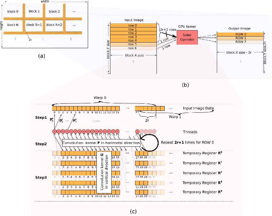
As shown in Fig. 2(a), the input image is evenly distributed to different blocks for parallel processing by the GPU. Each block is assigned multiple rows and columns of image data. Because the Sobel filter is a surrounding window centered on the target pixel, two adjacent blocks must have overlaps. When the radius of the filter is $r$ , the overlap between any two blocks is $2r$ .

4.3.2 Data Flow

For a large input image, assigning a thread to each pixel is expensive. Our strategy involves allocating sufficient threads in the horizontal direction while processing sequentially in the vertical direction. Moreover, because the Sobel operator does not require frequent data sharing between pixels, the shared memory is not used in our kernel. This avoids reducing block parallelism caused by excessive allocation of shared memory and reduces latency caused by memory accesses. Figure 2(b) shows the data flow of one block for filter $K_{x}$ . At the beginning, 2r+1 rows (5 rows for a $5\times{5}$ operator) of the input image are loaded into the kernel sequentially and processed to achieve the detection result of the rth row (ROW 0). Then, for each incremental row (ROW 1,2) in the output image, only the incremental parts of the input image (row 5,6) must be updated at a time. This is primarily because the filter $K_{x}$ can be decomposed into the product of the two vectors shown in Eq. 5, indicating that the calculations of the horizontal and vertical directions can be performed separately. Therefore, the intermediate results of the overlapping rows (rows 2 - 4) can be held in the kernel, and only incremental rows must be calculated each time. As mentioned, because each block has overlapping regions, the output image size is smaller than the input, with 2r fewer columns and rows in the horizontal and vertical directions, respectively.

4.3.3 Process Detail

Figure 2(c) shows the process detail of one warp for filter $K_{x}$ . The actions can be divided into three steps as follows.

•

Step 1: each thread loads the corresponding pixel data in one row from the global memory to the register, and then shares it with other threads within the same warp using the $\_\_shfl\_down\_sync$ primitive. Here, we define the $p_{i}^{j}$ to denote the obtained pixel data, where i denotes the thread ID and j denotes the pixel index. Because for a $5\times{5}$ filter, the upper bound of j is i+4, and data sharing between threads cannot cross the warp, the last four (2r) threads will be idle, which is the reason the overlap between blocks is 2r columns.
•

Step 2: after obtaining the necessary pixel data, each thread performs the basic convolution operations as follows:

$F_{i}^{u}=-1\cdot{p_{i}^{0}}+(-b)\cdot{p_{i}^{1}}+b\cdot{p_{i}^{3}}+p_{i}^{4},$ (6)

and stores result $F_{i}^{u}$ to the corresponding register $R_{i}^{u}$ , where u denotes the row index of the input image. Then, for the initial calculation, Steps 1 and 2 are repeated for 2r+1 times until all rows are calculated. Otherwise, only the oldest register data needs to be updated. Note that because our method is based on separable convolution, instead of expanding the calculation around a target pixel, thread i actually calculates the result of pixel i+r in each row.

•

Step 3: after completing horizontal calculations, each thread begins to perform the vertical convolution operations $G_{i}$ , whose equation can be expressed as follows:

	$\displaystyle G_{i}^{v}$	$\displaystyle=a\cdot{F_{i}^{f(v-2)}}+an\cdot{F_{i}^{f(v-1)}}+am\cdot{F_{i}^{f(v)}}$		(7)
		$\displaystyle+an\cdot{F_{i}^{f(v+1)}}+a\cdot{F_{i}^{f(v+2)}},$		(7)

where

f(x)=x\bmod{5},\hskip 14.22636ptx\geq{0}.

(8)

$f(x)$ is used to represent the row index because $F$ obtained by the Eq. 6 is dynamically updated. The $v$ in Eq. 7 denotes the index of the center row, always maintaining the variable $x$ greater than 0. Referring to the three steps, edge detection in the horizontal direction can be effectively implemented using the $5\times{5}$ Sobel filter $K_{x}$ . Similarly, detection using filter $K_{y}$ in the vertical direction can be implemented in the same manner, using different coefficients.

4.3.4 Optimization for Data Loading

Typically, the data loading of the increments and calculations can be sequentially alternated as shown in Fig. 3(a). Its benefit is in avoiding occupying too many on-chip registers, thereby reducing the thread parallelism. However, it also directly leads to frequent accesses to the global memory, which can generate a considerable latency. To solve this, we explicitly load the incremental image data from the global memory while calculating the on-chip data using the prefetching mechanism mentioned in Section 4.2. As shown in Fig. 3(b), after loading the fourth row, we continue with loading the fifth row without directly completing the calculations of G. Instead, these calculations will end while waiting for the loading to complete, which can help us achieve parallelism in time and significantly improve the efficiency of kernel execution. Here, because the prefetching trades more registers for time parallelism, to avoid additional burden to the processor, only one row of image data is fetched at a time. Thus, the row index function f(x) in Eq. 8 is changed to

f(x)=x\bmod{6},\hskip 14.22636ptx\geq{0},

(9)

when the prefetching mechanism is active.

4.3.5 Optimization for Diagonal Direction

According to Eq. 5, elements $k_{ij}$ of $K_{d}$ and $K_{dt}$ are neither symmetric nor proportional, which implies that they cannot be directly decomposed in the same manner as $K_{x}$ and $K_{y}$ . This also implies that the convolution results $F_{d}$ and $F_{dt}$ in horizontal cannot be reused and must be recalculated for each $G_{d}$ and $G_{dt}$ . To solve this, we propose a new idea to generate two matrices $K_{d+}$ and $K_{d-}$ as follows.

$\displaystyle K_{d+}$	$\displaystyle=K_{d}+K_{dt}$	(10)
	$\displaystyle=a\cdot{\begin{bmatrix}-m&-n-b&-2&-n-b&-m\\ b-n&-mb&-2nb&-mb&b-n\\ \textbf{0}&\textbf{0}&\textbf{0}&\textbf{0}&\textbf{0}\\ n-b&mb&2nb&mb&n-b\\ m&n+b&2&n+b&m\end{bmatrix}},$
$\displaystyle K_{d-}$	$\displaystyle=K_{d}-K_{dt}$
	$\displaystyle=a\cdot{\begin{bmatrix}-m&b-n&\textbf{0}&n-b&m\\ -n-b&-mb&\textbf{0}&mb&n+b\\ -2&-2nb&\textbf{0}&2nb&2\\ -n-b&-mb&\textbf{0}&mb&n+b\\ -m&b-n&\textbf{0}&n-b&m\end{bmatrix}},$

which satisfy the symmetry requirements by calculating the sum and difference of $K_{d}$ and $K_{dt}$ . If we efficiently use the two filters $K_{d+}$ and $K_{d-}$ , then $G_{d}$ and $G_{dt}$ are easily obtained as follows:

	$\displaystyle G_{d}$	$\displaystyle=K_{d}\ast{I}=\frac{K_{d}^{+}+K_{d}^{-}}{2}\ast{I}=\frac{G_{d}^{+}+G_{d}^{-}}{2},$		(11)
	$\displaystyle G_{dt}$	$\displaystyle=K_{dt}\ast{I}=\frac{K_{d}^{+}-K_{d}^{-}}{2}\ast{I}=\frac{G_{d}^{+}-G_{d}^{-}}{2}.$		(11)

For each row u, the convolution results $F_{ki}^{u}$ in the horizontal direction using filter $K_{d+}$ can be obtained as follows:

$\displaystyle F_{k0}^{u}$	$\displaystyle=-am\cdot{p^{0}}+a(-n-b)\cdot{p^{1}}+(-2a)\cdot{p^{2}}$	(12)
	$\displaystyle+a(-n-b)\cdot{p^{3}}+(-am)\cdot{p^{4}},$
$\displaystyle F_{k1}^{u}$	$\displaystyle=a(b-n)\cdot{p^{0}}+(-amb)\cdot{p^{1}}+(-2anb)\cdot{p^{2}}$
	$\displaystyle+(-amb)\cdot{p^{3}}+a(b-n)\cdot{p^{4}},$
$\displaystyle F_{k2}^{u}$	$\displaystyle=0,$
$\displaystyle F_{k3}^{u}$	$\displaystyle=a(n-b)\cdot{p^{0}}+(amb)\cdot{p^{1}}+(2anb)\cdot{p^{2}}$
	$\displaystyle+(amb)\cdot{p^{3}}+a(n-b)\cdot{p^{4}},$
$\displaystyle F_{k4}^{u}$	$\displaystyle=am\cdot{p^{0}}+a(n+b)\cdot{p^{1}}+(2a)\cdot{p^{2}}$
	$\displaystyle+a(n+b)\cdot{p^{3}}+(am)\cdot{p^{4}}.$

In addition, for a center row v, the results $G_{d+}^{v}$ can be obtained by aggregating the four $F_{ki}$ from adjacent rows as follows:

G_{d+}^{v}=F_{k0}^{v-2}+F_{k1}^{v-1}+F_{k3}^{v+1}+F_{k4}^{v+2},v\geq{2}.

(13)

Here, for the convenience of understanding, we use ki to represent the vector index in filter $K_{d+}$ , instead of using the thread index i in Eq. 6. Because the absolute values of the weights are symmetrical, for each row u, $F_{k3}^{u}$ and $F_{k4}^{u}$ are easily obtained using $F_{k1}^{u}$ and $F_{k0}^{u}$ :

	$\displaystyle F_{k3}^{u}$	$\displaystyle=F_{-k1}^{u}=-F_{k1}^{u},$		(14)
	$\displaystyle F_{k4}^{u}$	$\displaystyle=F_{-k0}^{u}=-F_{k0}^{u},$		(14)

and

G_{d+}^{v}=F_{k0}^{v-2}+F_{k1}^{v-1}-F_{k1}^{v+1}-F_{k0}^{v+2},v\geq{2}.

(15)

Thus, we effectively reuse part of the intermediate results, as shown in Fig. 4, without repeating convolution operations for each row. Figure 4(a) shows the procedure of $G_{d+}$ and Fig. 4(b) presents synchronous changes of on-chip register data. In Step 1, we use k1 to convolve the second row instead of k2, because k2 is a zero vector and does not affect the convolution result. This prepares the reused data required to ensure operation consistency in each step. Furthermore, we regard $F_{k3}^{3}$ and $F_{k4}^{4}$ as $F_{-k1}^{3}$ and $F_{-k0}^{4}$ , respectively, to be able to discover the pattern of data reuse. Then, $G_{d+}^{2}$ can be obtained according to Eq. 15 while loading the fifth row of the image. After it succeeds, the sixth row begins to be loaded. Simultaneously, the vectors from k0 to -k0 are strided down to convolve the rows centered on row 3. In Step 2, in addition to convolving the fifth row with -k0, only $F_{k0}^{1}$ and $F_{-k1}^{4}$ (green blocks) need to be recalculated because $F_{k1}^{2}$ can be reused. Compared with the original operations in Step 1, Step 2 significantly saves a quarter of the computation, ensuring that the filtering of $K_{d+}$ is efficiently performed. Note that after Step 3, the second vectors k1 used in each step are always the opposite of the previous step. However, this calculation can be reflected in the calculation of $G_{d+}$ without updating the register data. This method can be repeatedly applied to the calculation of incremental rows, while the register index of the latest row is dynamically updated according to Eq. 9.

For filter $K_{d-}$ , the $F_{ki}^{u}$ in the horizontal direction can be obtained as follows:

$\displaystyle F_{k0}^{u}$	$\displaystyle=-am\cdot{p^{0}}+a(b-n)\cdot{p^{1}}$	(16)
	$\displaystyle+a(n-b)\cdot{p^{3}}+(am)\cdot{p^{4}},$
$\displaystyle F_{k1}^{u}$	$\displaystyle=a(-n-b)\cdot{p^{0}}+(-amb)\cdot{p^{1}}$
	$\displaystyle+(amb)\cdot{p^{3}}+a(n+b)\cdot{p^{4}},$
$\displaystyle F_{k2}^{u}$	$\displaystyle=(-2a)\cdot{p^{0}}+(-2anb)\cdot{p^{1}}+2anb\cdot{p^{3}}+2a\cdot{p^{4}}$
$\displaystyle F_{k3}^{u}$	$\displaystyle=F_{k1}^{u}$
$\displaystyle F_{k4}^{u}$	$\displaystyle=F_{k0}^{u}.$

In addition, the $G_{d-}^{v}$ of a center row v can be obtained using Eq. 17:

G_{d-}^{v}=F_{k0}^{v-2}+F_{k1}^{v-1}+F_{k2}^{v}+F_{k1}^{v+1}+F_{k0}^{v+2},v\geq{2}.

(17)

Figure 5(a) shows the procedure of $G_{d-}$ , and Fig. 5(b) presents the changes of on-chip register data synchronously, which is the same method as $G_{d+}$ . According to this figure, all convolutions for each row must be recalculated in each step because the $K_{d-}$ filter no longer has a zero vector in the horizontal direction, missing buffers that can be reused.

Inspired by Eq. 5, we decompose $K_{d-}$ into the sum of two products of two vectors as follows:

$\displaystyle K_{d-}$	$\displaystyle=a\cdot{\begin{bmatrix}-m&b-n&\textbf{0}&n-b&m\\ -n-b&-mb&\textbf{0}&mb&n+b\\ -2&-2nb&\textbf{0}&2nb&2\\ -n-b&-mb&\textbf{0}&mb&n+b\\ -m&b-n&\textbf{0}&n-b&m\end{bmatrix}}$	(18)
$\displaystyle=$	$\displaystyle a\cdot\biggl(\begin{bmatrix}m\\ n+b\\ 2\\ n+b\\ m\end{bmatrix}\times{\begin{bmatrix}-1&-b&\textbf{0}&b&1\end{bmatrix}}$
	$\displaystyle-\begin{bmatrix}mb+b-n\\ nb+b^{2}-mb\\ 2b-2nb\\ nb+b^{2}-mb\\ mb-n+b\end{bmatrix}\times{\begin{bmatrix}0&-1&\textbf{0}&1&0\end{bmatrix}}\biggr).$

Equation 18 demonstrates that the first $1\times{5}$ horizontal vector is the same as $K_{x}$ , which means that its intermediate results can be reused without recalculation. In addition, the second horizontal vector means we only need to calculate the difference between columns 2 and 4. Thus, the $G_{d-}^{v}$ of a center row v is easily obtained as follows:

$\displaystyle G_{d-}^{v}$	$\displaystyle=am\cdot{F^{f(v-2)}}+a(n+b)\cdot{F^{f(v-1)}}+2a\cdot{F^{f(v)}}$	(19)
	$\displaystyle+a(n+b)\cdot{F^{f(v+1)}}+am\cdot{F^{f(v+2)}}$
	$\displaystyle-a(mb+b-n)\cdot{D^{f(v-2)}}-a(nb+b^{2}-mb)\cdot{D^{f(v-1)}}$
	$\displaystyle-a(2b-2nb)\cdot{D^{f(v)}}-a(nb+b^{2}-mb)\cdot{D^{f(v+1)}}$
	$\displaystyle-a(mb-n+b)\cdot{D^{f(v+2)}},$

and

f(x)=x\bmod{6},\hskip 14.22636ptx\geq{0},

where $D$ denotes the convolution results under the second horizontal vector. Therefore, although the on-chip registers must still be updated every time, we only need to perform simple multiply-accumulate operations instead of multiple convolutions, significantly reducing the overall calculation amount and improving the processing speed.

Thus far, the efficient calculation methods in all four directions for a $5\times{5}$ Sobel operator have been introduced, and the final edge detection result can be obtained by integrating the respective results in these four directions according to Eq. 4.

Table 1: Speed performance of our four-directional Sobel operators.

			Execution time (µs)							Throughput(GB/s)
Hardware	Sobel operator	Image size	GM	SM	SM-P	RG	RG-v1	RG-v2	IO	HToD	DToH	Speedup
GTX1650Ti		$512\times{512}$	10.285	14.626	14.246	6.766	-	-	80.475	6.035	6.233	1.52
	$3\times{3}$	$1024\times{1024}$	43.792	55.639	54.455	30.791	-	-	316.52	6.115	6.287	1.42
		$2048\times{2048}$	165.86	206.81	198.71	105.22	-	-	1263.9	6.151	6.254	1.576
		$512\times{512}$	29.712	30.913	28.606	24.905	20.884	18.747	80.475	6.035	6.223	1.585
	$5\times{5}$	$1024\times{1024}$	124.00	109.59	107.78	95.940	77.918	66.225	316.52	6.115	6.287	1.872
		$2048\times{2048}$	424.37	418.50	411.91	350.36	286.01	249.22	1263.9	6.151	6.254	1.702
Jetson AGX		$512\times{512}$	17.426	17.693	17.139	13.881	-	-	17.049	26.512	34.488	1.255
	$3\times{3}$	$1024\times{1024}$	60.748	59.483	60.975	37.816	-	-	65.737	28.802	32.440	1.606
		$2048\times{2048}$	250.65	230.66	227.94	160.81	-	-	914.23	10.504	7.501	1.559
		$512\times{512}$	48.625	34.739	34.379	31.346	28.118	26.620	17.049	26.512	34.488	1.827
	$5\times{5}$	$1024\times{1024}$	164.41	141.66	120.68	116.14	115.06	93.354	65.737	28.802	32.440	1.761
		$2048\times{2048}$	694.99	572.95	549.38	499.15	454.63	368.24	914.23	10.504	7.501	1.887

(a) AGX global memory

(b) 1650Ti: global memory

(d) 1650Ti: global memory

(e) AGX: shared memory

(f) 1650Ti: shared memory

(g) AGX: shared memory

(h) 1650Ti: shared memory

(i) AGX: register

(j) 1650Ti: register

(k) AGX: register

(l) 1650Ti register

Figure 6: Speed comparison of four-directional Sobel operators for a

1024\times{1024}

image in different resource configurations.

Table 2: Speed comparisons of two-directional Sobel operators with other methods.

Method	Operator size	Image size	Runtime^∗ (ms)	Hardware	MPS	MPS/C
SobelGPU-Jetson	$3\times{3}$	$1024\times{1024}$	0.074	Jetson AGX	1.41E10	2.77E7
		$2048\times{2048}$	0.519		8.07E9	1.58E7
	$5\times{5}$	$1024\times{1024}$	0.085		1.24E10	2.42E7
		$2048\times{2048}$	0.552		7.59E9	1.48E7
SobelGPU-GTX	$3\times{3}$	$1024\times{1024}$	0.190	GTX 1650Ti	5.51E9	5.38E6
		$2048\times{2048}$	0.740		5.66E9	5.53E6
	$5\times{5}$	$1024\times{1024}$	0.199		5.27E9	5.14E6
		$2048\times{2048}$	0.763		5.49E9	5.36E6
OpenCV-GPU 1	$3\times{3}$	$1024\times{1024}$	0.512	Jetson AGX	2.05E9	4E6
		$2048\times{2048}$	1.778		2.36E9	4.6E6
	$5\times{5}$	$1024\times{1024}$	0.566		1.85E9	3.62E6
		$2048\times{2048}$	1.832		2.29E9	4.47E6
OpenCV-GPU 2	$3\times{3}$	$1024\times{1024}$	2.43	GTX 1650Ti	4.31E8	4.21E5
		$2048\times{2048}$	9.82		4.27E8	4.18E5
	$5\times{5}$	$1024\times{1024}$	2.53		4.14E8	4.05E5
		$2048\times{2048}$	9.90		4.24E8	4.14E5
Xiao [13]	$3\times{3}$	$1024\times{1024}$	5.48^†	GTX 1070	1.91E8	9.97E4
		$2048\times{2048}$	18.95^†		2.21E8	1.15E5
Zahra [22]	$3\times{3}$	$512\times{512}$	3.62	GTX 550Ti	7.24E7	3.77E5
		$1024\times{1024}$	14.74		7.11E7	3.7E5
Theodora [23]	$3\times{3}$	$1024\times{1024}$	0.601	GTX 1060	1.74E9	1.36E6
		$2048\times{2048}$	0.926		4.52E9	3.53E6
	$5\times{5}$	$1024\times{1024}$	0.837		1.25E9	9.79E5
		$2048\times{2048}$	1.174		3.57E9	2.79E6
Dore [24]	$3\times{3}$	$1024\times{1024}$	11.01^†	GTX 470	9.5E7	2.1E5
		$2048\times{2048}$	84.023^†		5E7	1.1E5
You [25]	$3\times{3}$	$1024\times{768}$	5	DE1-SoC	1.57E8	-
		$1920\times{1080}$	15		1.38E8	-
Sato [26]	$3\times{3}$	$512\times{512}$	1.1	Cyclone II	2.38E8	-
		$1024\times{1024}$	4.37		2.39E8	-
Tim [27]	$3\times{3}$	$1280\times{1024}$	31	ZYNQ 7030	4.22E7	-

1

*: Runtime includes the kernel execution time and data loading time. ^†: Only the kernel execution time is included.

5 Evaluation and Discussion

5.1 Evaluation Platforms

We implemented our multi-directional 5 $\times$ 5 Sobel operator kernel on an embedded Jetson AGX Xavier GPU and Nvidia GTX 1650Ti mobile GPU, because as widely used mobile GPUs, they have recently been used in some studies to handle systems that combine Sobel operators with other upper-layer applications [19] [20] [21]. At the same time, these two kinds of GPUs have different architectures, which determine that the same CUDA kernel often reflects utterly different performance. Jetson AGX Xavier is a powerful platform, built on an Nvidia Volta GPU with 512 cores and shares physical memory with the center processor. Users can allow both the host and device to access the shared data by applying for managed memory, reducing the impact of data transmission. In contrast, the GTX 1650Ti is built on a Turing architecture with 1024 cores and has dedicated memory. Although it has a higher calculation capability than Jetson AGX Xavier, the data it processes must be first transferred from the host memory to the device memory through the PCIe bus, which increases the burden of IO. Evaluating our kernel on both platforms helps us fully understand its performance, and users can choose different solutions according to their requirements.

5.2 Evaluation of Kernel Performance

We evaluated the performance using three different sizes of images: 512 $\times{512}$ , $1024\times 1024$ , and $2048\times{2048}$ . To evaluate kernel performance more comprehensively, we used global and shared memory as storage mediums other than the register. Additionally, we compared the 3 $\times$ 3 operator.

Table 1 lists the speed performance of our four-directional kernels. GM, SM, and RG represent the original methods using global memory, shared memory, and registers, respectively. SM-P represents the method that covers transmission latency by adding the prefetching mechanism to SM. RG-v1 indicates that we transformed the original diagonal filters $K_{d}$ and $K_{dt}$ into $K_{d+}$ and $K_{d-}$ ; and RG-v2 the method that further decomposes $K_{d-}$ based on RG-v1. All RG series kernels are equipped with the prefetching mechanism. Because the calculation of the 3 $\times$ 3 operator in the diagonal directions is not complicated, we only perform RG-v1 and RG-v2 to the 5 $\times$ 5 operator. Speedup denotes the ratio of GM to RG at runtime. For each kernel, we used the NVprof profiling tool to measure the kernel execution time 100 times and took the average value as the final execution time. Also, we calculated the standard deviation of the execution time of each kernel, ranging from 0.06 to 5.05, which fully proves the robustness of our measurement results. Regardless of the platform, our kernel achieved a 1.3x speedup, and the maximum even reached over 1.8x. For the degraded case, the SM series kernels on a GTX 1650Ti are slower than those of GM. This is because using the shared memory without optimization only increases data transmission costs and reduces kernel performance. Although using the prefetching mechanism can hide latency and reduce the execution time by 19µs on average compared with GM, the performance of SM-P for a 3 $\times$ 3 operator on GTX 1650Ti is still lower than that of GM. This implies that, for a 3 $\times$ 3 operator, using shared memory as the storage medium is not a good choice. The execution time of the kernels increases linearly with the image size on both platforms: approximately 4x on both platforms. This steady change indirectly indicates that our method can fully utilize hardware resources. Additionally, in almost all cases, the introductions of SM-P, RG-v1 and RG-v2 gradually introduce a reduction in execution time, indicating that our proposed methods are effective and have high robustness. Particularly for the 5 $\times$ 5 operator, the speed of our accelerated kernel RG-v2 (66.225µs) is only 33% slower than the original 3 $\times$ 3 kernel GM (43.792µs), enabling us to use the 5 $\times$ 5 Sobel operator with higher detection precision instead of 3 $\times$ 3 in the future. IO denotes the data transmission time required according to the hardware architecture. As mentioned, because Jetson AGX Xavier GPU shares the physical memory between the GPU and CPU, it does not cost too much on IO. By contrast, the IO costs required on GTX 1650Ti are much higher than the kernel execution. The Throughput metrics between the host and the device in both directions also reflect the same issue. The throughputs we achieved on Jetson AGX Xavier are much higher than those of GTX 1650Ti, but still far from theoretical values. This means that our kernel is memory limited and could be further ameliorated by processing larger images or video streams.

Because our kernel is implemented in CUDA, the block size configuration is closely related to its performance. Therefore, we provide different combinations of block configurations to the kernels and perform the 3 $\times$ 3 and 5 $\times$ 5 four-directional Sobel operators on the 1024 $\times$ 1024 image shown in Fig. 6. Each row of graphs represents different storage mediums used in our kernels. The graphs in columns 1 and 2 show the processing results of the 3 $\times$ 3 operator under different block configurations and platforms, and columns 3 and 4 show those for 5 $\times$ 5. In each sub-graph, the x-axis represents the number of grid.y, which is determined by the number of image sizes and threads allocated in the y direction within each block; the larger the number, the fewer rows each block processes in the y-axis direction. The y-axis represents the execution time of these kernels. The methods performed here are the same as those tested in Table 1. The difference is that we specified block1: (128,1) and block2: (256,1) configurations for each method. According to the results, block1 and block2 do not affect much under the same method in most cases. Moreover, the speed relationship between these methods is the same as that shown in Table 1. Therefore, we predict that the individual difference is caused by changes in thread parallelism resulting from different register usage rates. For each method, a large grid.y typically shows a high performance because a higher number of blocks indicates a more significant number of active blocks in parallel. Thus, the kernel can use hardware resources better, resulting in better performance.

Table 2 shows the speed comparison of our kernel with other methods in two directions. The comparison objects are fast Sobel operators published in recent years, and each study provides their operator sizes, image sizes, execution time, and required hardware platforms. Here, Runtime includes the kernel execution time and data loading time from the host memory to the device. The hardware used by these studies is primarily divided into two categories: GPUs and field programmable gate arrays (FPGAs). Both are the most widely used algorithm accelerators today. To compare the computing capability of these operators based on different hardware, we list the mega-pixel per second (MPS) values of all these studies. Additionally, we use the mega-pixel per second per core (MPS/C) parameter, which represents the number of pixels processed per second by each core, to normalize their processing capabilities on different GPUs. According to the Runtime, our kernels based on AGX are faster than those based on 1650Ti, contrary to the results shown in Table 2. This is because of the considerable time required by the IO, resulting in a decrease in overall throughput. Compared with other studies, our operators are much faster in each case. Particularly for OpenCV-GPU, the most commonly used method in image edge detection, the processing speed is approximately 3.3x to 13.3x slower than our kernels. This is because the OpenCV-GPU treads the Sobel operator as a 2D convolution filter by default, and ours is actually further optimized on the basis of two 1D separable kernels. Besides, the OpenCV-GPU does not provide the functions in the diagonal directions, where our kernel has a considerable advantage. Xiao [13], Zahra [22], and Dore [24] implemented their fast 3 $\times$ 3 Sobel operators on GPUs, and You [25], Sata [26], and Tim [27] implemented on FPGAs. They all achieved real-time processing on a large-scale image, but remain at the milliseconds level, leaving little processing time for upper-layer applications. Theodora [23] implemented a complete version evaluation, including the combination of two Sobel operators and two images of different sizes. Their execution times are approximately 1.3x to 4.2x longer than ours, even using a GTX 1060 GPU superior to our GTX 1650Ti. According to the MPS and MPS/C, our numbers exceed those of other studies, demonstrating that our kernels have an overwhelming advantage.

To confirm the correctness, we listed edge detection results of four images shown in Fig. 7. For each image, we perform the edge detection using four different GPU kernels, including the two-directional OpenCV-GPU kernel (Fig. 7(b)); our two-directional RG kernel (Fig. 7(c)); our four-directional GM kernel (Fig. 7(d)) and our four-directional RG-v2 kernel (Fig. 7(e)). All the sizes of kernels are 5 $\times$ 5. Here, because kernels (b) and (d) are implemented by the most primitive method, we take them as reference objects, and calculate the Structure Similarity Index Measure (SSIM) values of (c) and (e) relative to them respectively. SSIM is an indicator to measure the similarity of two images, and is calculated from the three image features of luminance, contrast and structure. It can be calculated as follow:

\displaystyle SSIM(x,y)

\displaystyle=\frac{(2\mu_{x}\mu_{y}+C_{1})(2\sigma_{xy}+C_{2})}{(\mu_{x}^{2}+\mu_{y}^{2}+C_{1})(\sigma_{x}^{2}+\sigma_{y}^{2}+C_{2})}.

(20)

Here, $\mu$ and $\sigma^{2}$ represent the mean value and variance of the image, respectively, and $\sigma_{xy}$ represents the covariance between the image x and image y. Finally, $C_{1}$ and $C_{2}$ are two constants used to avoid instability when $\mu_{x}^{2}+\mu_{y}^{2}$ or $\sigma_{x}^{2}+\sigma_{y}^{2}$ are close to zero. The closer SSIM to 1 indicates, the higher the similarity of two images. According to the high SSIM values of 0.99 shown in Fig. 7, it can be observed that the proposed acceleration method can guarantee the correctness of Sobel operators in both two and four directions.

6 Conclusion

This paper proposed a fast GPU kernel for a four-directional $5\times{5}$ Sobel operator that entirely uses the register resource. We improved the Sobel operator from two perspectives: computer architecture and mathematics. In computer architecture, we focused on fully using registers with the help of warp-level primitives without utilizing global memory and shared memory. Simultaneously, we introduced the prefetching mechanism to hide the system latency caused by data transmission. Concerning mathematics, we proposed a two-step optimization method for the Sobel operator with complex patterns in diagonal directions, enabling us to fully reuse intermediate results and significantly improve the execution efficiency of the kernel. Extensive experiments prove that our kernel has high robustness, with significant improvements in detection speed for images of different sizes. Furthermore, our kernel achieves 6.7x and 13x improvements in processing speed compared with the OpenCV-GPU library on two different GPUs. To the best of our knowledge, the proposed kernel is currently the fastest kernel based on GPUs.

To further facilitate our kernel’s application, we plan to combine it with high-level applications such as object detection. In addition, for the bottleneck problem of IO, we predict that stream processing can efficiently reduce the latency caused by data transmission. In addition, the burden of on-chip computation not being too heavy must be ensured. These concerns will be addressed in future work.

CRediT Author Statement

Qiong Chang: algorithm design, basic code writing, experiment design, draft manuscript writing. Xiang Li: code optimization, experiment, manuscript co-writing. Yun Li: supervision, experiment environment preparation, writing-reviewing. Jun Miyazaki: supervision, writing-reviewing and editing. All authors contributed to discussions. Qiong Chang and Xiang Li contributed equally to this work.

Conflict of interest

The authors declare that they have no conflict of interest.

References

[1] Ping, Bo, Fenzhen Su, and Yunyan Du. ”Bohai front detection based on multi-scale Sobel algorithm.” 2014 IEEE Geoscience and Remote Sensing Symposium. IEEE, 2014.
[2] AS, Remya Ajai, and Sundararaman Gopalan. ”Comparative Analysis of Eight Direction Sobel Edge Detection Algorithm for Brain Tumor MRI Images.” Procedia Computer Science 201 (2022): 487-494.
[3] Biswas, Soumen, and Dibyendu Ghoshal. ”Blood cell detection using thresholding estimation based watershed transformation with Sobel filter in frequency domain.” Procedia Computer Science 89 (2016): 651-657.
[4] Abdullah, S. Sheik, and M. Pallikonda Rajasekaran. ”Modified Sobel mask to locate knee joint boundaries.” 3C Tecnología. G losas De innovaci on Aplicadas a La Pyme (2020): 195-205.
[5] AS, Remya Ajai, and Sundararaman Gopalan. ”Comparative Analysis of Eight Direction Sobel Edge Detection Algorithm for Brain Tumor MRI Images.” Procedia Computer Science 201 (2022): 487-494.
[6] Jing, Min, and Yubo Du. ”Flank angle measurement based on improved Sobel operator.” Manufacturing Letters 25 (2020): 44-49.
[7] Chen, Siyu, et al. ”Innovation of aggregate angularity characterization using gradient approach based upon the traditional and modified Sobel operation.” Construction and Building Materials 120 (2016): 442-449.
[8] Li, Zhihao, et al. ”Efficient parallel optimizations of a high-performance SIFT on GPUs.” Journal of Parallel and Distributed Computing 124 (2019): 78-91.
[9] Chang, Qiong, et al. ”Efficient stereo matching on embedded GPUs with zero-means cross correlation.” Journal of Systems Architecture 123 (2022): 102366.
[10] Mohamed, Mohammed, and Gita Alaghband. ”An Improved Parallel Eight Direction Prewitt Edge Detection Algorithm.” Proceedings of the International Conference on Image Processing, Computer Vision, and Pattern Recognition (IPCV). The Steering Committee of The World Congress in Computer Science, Computer Engineering and Applied Computing (WorldComp), 2013.
[11] Jo, Ji Hoon, and Sang Gu Lee. ”Sobel Mask Operations Using Shared Memory in CUDA Environment.” 2012 6th International Conference on New Trends in Information Science, Service Science and Data Mining (ISSDM2012). IEEE, 2012.
[12] Chouchene, Marwa, et al. ”Efficient implementation of Sobel edge detection algorithm on CPU, GPU and FPGA.” International Journal of Advanced Media and Communication 5.2-3 (2014): 105-117.
[13] Xiao, Han, et al. ”Image Sobel edge extraction algorithm accelerated by OpenCL.” The Journal of Supercomputing (2022): 1-30.
[14] Zuo, H. R., et al. ”Fast sobel edge detection algorithm based on GPU.” Opto-Electronic Engineering 36.1 (2009): 41-43.
[15] Sobel, Irwin, and Gary Feldman. ”A 3x3 isotropic gradient operator for image processing.” A talk at the Stanford Artificial Project in (1968): 271-272.
[16] NVIDIA corporation: NVIDIA CUDA C programming guide, 2022, Version 11.7.0.
[17] Chang, Qiong, Masaki Onishi, and Tsutomu Maruyama. ”Fast convolution Kernels on Pascal GPU with High Memory Efficiency.” Proceedings of the High Performance Computing Symposium. 2018.
[18] Chang, Qiong, and Tsutomu Maruyama. ”Real-Time High-Quality Stereo Matching System on a GPU.” 2018 IEEE 29th International Conference on Application-specific Systems, Architectures and Processors (ASAP). IEEE, 2018.
[19] Beleznai, Csaba, et al. ”Pose-aware object recognition on a mobile platform via learned geometric representations.” 2022 13th Asian Control Conference (ASCC). IEEE, 2022.
[20] Verucchi, Micaela, et al. ”Real-Time clustering and LiDAR-camera fusion on embedded platforms for self-driving cars.” 2020 Fourth IEEE International Conference on Robotic Computing (IRC). IEEE, 2020.
[21] Taspinar, Yavuz Selim, Murat Koklu, and Mustafa Altin. ”Fire Detection in Images Using Framework Based on Image Processing, Motion Detection and Convolutional Neural Network.” International Journal of Intelligent Systems and Applications in Engineering 9.4 (2021): 171-177.
[22] Emrani, Zahra, Soroosh Bateni, and Hossein Rabbani. ”A new parallel approach for accelerating the gpu-based execution of edge detection algorithms.” Journal of Medical Signals and Sensors 7.1 (2017): 33.
[23] Sanida, Theodora, Argyrios Sideris, and Minas Dasygenis. ”A Heterogeneous Implementation of the Sobel Edge Detection Filter Using OpenCL.” 2020 9th International Conference on Modern Circuits and Systems Technologies (MOCAST). IEEE, 2020.
[24] Dore, Aruna, and Sunitha Lasrado. ”Performance analysis of Sobel edge filter on heterogeneous system using OpenCL.” International Journal of Research in Engineering and Technology 3.15 (2014): 53-57.
[25] You, Baoshan, et al. ”Implementation of Sobel Edge Detection on FPGA Based on OpenCL.” 2017 IEEE 7th Annual International Conference on CYBER Technology in Automation, Control, and Intelligent Systems (CYBER). IEEE, 2017.
[26] Sato, Tercio Naoki, Gabriel Pedro Krupa, and Leonardo Breseghello Zoccal. ”Performance Measurements of Sobel Edge Detection Implemented in an FPGA Architecture and Software.” Brazilian Technology Symposium. Springer, Cham, 2018.
[27] Chisholm, Tim, Romulo Lins, and Sidney Givigi. ”FPGA-based design for real-time crack detection based on particle filter.” IEEE Transactions on Industrial Informatics 16.9 (2019): 5703-5711.