Temporal Subsampling Diminishes Small Spatial Scales in Recurrent Neural Network Emulators of Geophysical Turbulence
Abstract
The immense computational cost of traditional numerical weather and climate models has sparked the development of machine learning (ML) based emulators. Because ML methods benefit from long records of training data, it is common to use datasets that are temporally subsampled relative to the time steps required for the numerical integration of differential equations. Here, we investigate how this often overlooked processing step affects the quality of an emulator’s predictions. We implement two ML architectures from a class of methods called reservoir computing: (1) a form of Nonlinear Vector Autoregression (NVAR), and (2) an Echo State Network (ESN). Despite their simplicity, it is well documented that these architectures excel at predicting low dimensional chaotic dynamics. We are therefore motivated to test these architectures in an idealized setting of predicting high dimensional geophysical turbulence as represented by Surface Quasi-Geostrophic dynamics. In all cases, subsampling the training data consistently leads to an increased bias at small spatial scales that resembles numerical diffusion. Interestingly, the NVAR architecture becomes unstable when the temporal resolution is increased, indicating that the polynomial based interactions are insufficient at capturing the detailed nonlinearities of the turbulent flow. The ESN architecture is found to be more robust, suggesting a benefit to the more expensive but more general structure. Spectral errors are reduced by including a penalty on the kinetic energy density spectrum during training, although the subsampling related errors persist. Future work is warranted to understand how the temporal resolution of training data affects other ML architectures.
Cooperative Institute for Research in Environmental Sciences (CIRES) at the University of Colorado Boulder, Boulder, CO, USA Physical Sciences Laboratory (PSL), National Oceanic and Atmospheric Administration (NOAA), Boulder, CO, USA Sofar Ocean, San Francisco, CA, USA University of California San Diego (UCSD), La Jolla, CA, USA Pacific Northwest National Laboratory, Richland, WA, USA
keypoints
Reducing training data temporal resolution by subsampling leads to overly dissipative small spatial scales in neural network emulators A quadratic autoregressive architecture is shown to be inadequate at capturing small scale turbulence, even when data are not subsampled Subsampling bias in Echo State Networks is mitigated but not eliminated by prioritizing kinetic energy spectrum during trainingPlain Language Summary
The computer models that govern weather prediction and climate projections are extremely costly to run, causing practitioners to make unfortunate tradeoffs between accuracy of the physics and credibility of their statistics. Recent advances in machine learning have sparked the development of neural network-based emulators, i.e., low-cost models that can be used as drop-in replacements for the traditional expensive models. Due to the cost of storing large weather and climate datasets, it is common to subsample these fields in time to save disk space. This subsampling also reduces the computational expense of training emulators. Here, we show that this pre-processing step hinders the fidelity of the emulator. We offer one method to mitigate the resulting errors, but we suggest that more research is needed to understand and eventually overcome them.
1 Introduction
Weather and climate prediction requires the numerical integration of one or more computational models derived from the fundamental equations of motion and initialized with an estimate of the present-day system state (e.g., temperature, wind speeds, etc.). Due to the high cost of these computational models, prediction systems typically require suboptimal tradeoffs. On one hand, it is desirable to increase the credibility of the underlying numerical model as much as possible, for instance by increasing model grid resolution (<)e.g.,¿[]hewitt_impact_2016 or by explicitly simulating as many coupled components (e.g., atmosphere, land, ocean, ice) as possible (<)e.g.,¿[]penny_coupled_2017. On the other hand, knowledge of the model initial conditions is imperfect and the governing equations will always contain necessary, inexact approximations of reality. As a result, prediction systems employ statistical methods like ensemble based forecasting in order to represent this uncertainty. Producing an ensemble with statistical significance requires integrating the underlying numerical model many times; usually in practice, but ideally or greater (Evensen et al. (2022)). Therefore, the resulting computational costs require practitioners to compromise between the fidelity of the numerical model and credibility of the statistical method.
An ongoing area of research that aims to enable statistical forecasting subject to the dynamics of an expensive numerical model is surrogate modeling. The general approach relies on using a model that represents or “emulates” the dynamics of the original numerical model with “sufficient accuracy” for the given application, while being computationally inexpensive to evaluate. Historically, surrogate models have been an important tool for nonlinear optimization (<)e.g.,¿[]li_data-based_2019,bouhlel_scalable_2020, and in the Earth sciences have been developed with techniques such as Linear Inverse Models (<)e.g., principal oscillation or interaction patterns;¿[]hasselmann_pips_1988,penland_random_1989, moore_linear_2022, kriging (Cressie (1993)), or polynomial chaos techniques (Najm (2009)), to name only a few. More recently, advances in computing power, the rise of general purpose graphics processing units, and the explosion of freely available data has encouraged the exploration of more expensive machine learning methods like neural networks for the emulation task (Schultz et al. (2021)). A number of data-driven, neural network architectures have been developed to generate surrogate models for weather forecasting and climate projection applications. Some examples include models based on feed forward neural networks (Dueben & Bauer (2018)), convolutional neural networks (<)CNNs;¿[]scher_toward_2018,scher_weather_2019,rasp_data-driven_2021,weyn_can_2019,weyn_improving_2020,weyn_sub-seasonal_2021, recurrent neural networks (<)RNNs;¿[]arcomano_machine_2020,chen_predicting_2021,nadiga_reservoir_2021, graph neural networks (Keisler (2022); Lam et al. (2022)), Fourier neural operators (Pathak et al. (2022)), and encoder-transformer-decoder networks (Bi et al. (2023)).
A significant advancement in surrogate modeling for weather and climate prediction has been the rapid increase in spatial resolution. To the best of our knowledge, the current highest resolution neural network emulators for global atmospheric dynamics is (31 km) (Pathak et al. (2022); Bi et al. (2023); Lam et al. (2022)), which is the same resolution as the ERA5 Reanalysis (Hersbach et al. (2020)) used to train these models. At this resolution, General Circulation Models (GCMs) of the atmosphere are capable of explicitly capturing important small scale processes like low-level jets and interactions with mountainous topography (Orlanski (1975)). However, it is not yet clear that neural networks are able to represent the same dynamical processes as the training data. Instead, based on our own experimentation, we hypothesize that without careful architectural modifications, neural network emulators will effectively operate at a coarser resolution than the original dataset used in training.

To make the discussion concrete, we present a sample prediction from our own surrogate model in Figure 1. The panels show the time evolution of Sea Surface Temperature (SST) in the Gulf of Mexico at 1/25∘ horizontal resolution, using data from a Navy HYCOM, 3D-Var-based reanalysis product as “Truth” (upper row; see Appendix B for data details). We generate the prediction (middle row) with an RNN architecture described more fully in Section 3.4. Generally speaking, the RNN captures the largest scales of the SST pattern over a 36 hour window. However, as time progresses, the SST pattern becomes overly smooth. The RNN is unable to capture the spatial details that are well resolved in the reanalysis dataset, with the largest errors evolving along sharp SST fronts. We note that a similar smoothing behavior can be observed in other neural network based emulators, see for example (<)¿[Figure 3]bi_accurate_2023, (<)¿[Figure 4c & 4d]pathak_fourcastnet_2022, (<)¿[Figure 5]keisler_forecasting_2022.
There are a number of reasons that could cause this smoothing behavior to manifest in the predictions. As we show in Sections 4 and 5, the blurring of small scale features is a high frequency spectral bias, which has been studied in relation to the training of feedforward neural networks (Xu et al. (2022)) and numerical instabilities of neural network predictions for turbulent flows (Chattopadhyay & Hassanzadeh (2023)). One potential reason that we observe spectral bias in our predictions is that the training uses a mean-squared error loss function, which is known to prioritize large over small scale features (Rossa et al. (2008)). Here, we suggest that any blurring effect from such a loss function is exacerbated by more fundamental decisions in the experimental design. Our primary goal is to explore how temporal subsampling in the training dataset adds to this blurring effect. We are motivated to study the impact of this subsampling because many existing emulators, including our example in Figure 1, rely on reanalysis products as training data (<)e.g.¿[]lam_graphcast_2022,bi_accurate_2023,pathak_fourcastnet_2022,keisler_forecasting_2022,weyn_sub-seasonal_2021,arcomano_machine_2020. While there are excellent reasons to leverage the existence of reanalysis products, namely that they are constrained to observational data, the shear size of the data requires some degree of temporal subsampling. We suggest that it is important to understand how this highly routine data reduction step impacts the performance of data-driven prediction methods when used for training.
In our work, we explore the degree to which temporal subsampling impedes single layer autogregressive and recurrent neural network emulators from learning the true underlying dynamics of the system. In order to isolate this effect from the potential impacts of a data assimilation system and multivariate interactions, we do not rely on the Gulf of Mexico reanalysis data. Instead, we use a model for Surface Quasi-Geostrophic (SQG) turbulence (Held et al. (1995); Blumen (1978)), which additionally gives us direct control over the datasets used for training, validation, and testing. The SQG model and dataset generation is described more fully in Section 2.
The architectures that we use in this study stem from a broad class of machine learning techniques termed as reservoir computing (RC), which was independently discovered as Echo State Networks (<)ESNs;¿[]jaeger_echo_2001, Liquid State Machines (Maass et al. (2002)), and the Decorrelation Backpropagation Rule (Steil (2004)). One defining characteristic of RC models is that all internal connections are adjusted by global or “macro-scale” parameters, significantly reducing the number of parameters that need to be trained. The relatively simplified structure and training requirements of RC make it an attractive architecture for large scale prediction because it enables rapid development, and could be useful in situations requiring online learning. More importantly though, we are motivated to use RC because past studies have repeatedly shown that it can emulate low dimensional chaotic systems while often outperforming more complex RNNs such as those with Long Short-Term Memory units (LSTMs) (<)e.g.¿[]platt_systematic_2022,vlachas_backpropagation_2020,griffith_forecasting_2019,lu_attractor_2018,pathak_model-free_2018. Additionally, Penny et al. (2022) showed that RC can be successfully integrated with a number of data assimilation algorithms, either by generating samples for ensemble based methods like the Ensemble Kalman Filter, or by generating the tangent linear model necessary for 4D-Var. Finally, we note that Gauthier et al. (2021) proposed a further simplification to the RC architecture based on insights from Bollt (2021) that unifies versions of RC with nonlinear vector autoregression (NVAR). For a variety of chaotic systems, this architecture has shown excellent prediction skill even with low order, polynomial-based feature vectors (T-C. Chen et al. (2022); Barbosa & Gauthier (2022); Gauthier et al. (2021)), despite requiring a much smaller hidden state and less training data. Considering all of these advancements, we are motivated to use these simple yet powerful single layer NVAR and ESN architectures to emulate turbulent geophysical fluid dynamics, and study how they are affected by temporal subsampling (see Section 3 for architecture details).
2 Surface Quasi-Geostrophic Turbulence
Our goal in this study is to emulate turbulent motions relevant to realistic geophysical fluid dynamics, while avoiding the complications associated with the data assimilation system used to produce reanalysis datasets, including observational noise and error covariance estimates, and the intricate multivariate interactions inside atmosphere or ocean GCMs. Therefore, we aim to emulate a numerical model for SQG turbulence (Held et al. (1995); Blumen (1978)) as outlined by Tulloch & Smith (2009). The model is formulated to represent the nonlinear Eady problem (Eady (1949)), following Blumen (1978). The model simulates turbulence on an plane with uniform stratification and shear, bounded by rigid surfaces km apart. The motion is determined entirely by temperature advection on the boundaries as follows,
where km is the surface layer of the atmosphere, and km is approximately at the top of the troposphere. Here, hatted variables denote spectral components, is the Jacobian in spectral space, and the temperature streamfunction is
with as the nondimensional wavenumber. We note that this model produces an approximate spectrum of without any break (Figure 2), as is expected in Eady turbulence. For more details on this model, see Tulloch & Smith (2009).
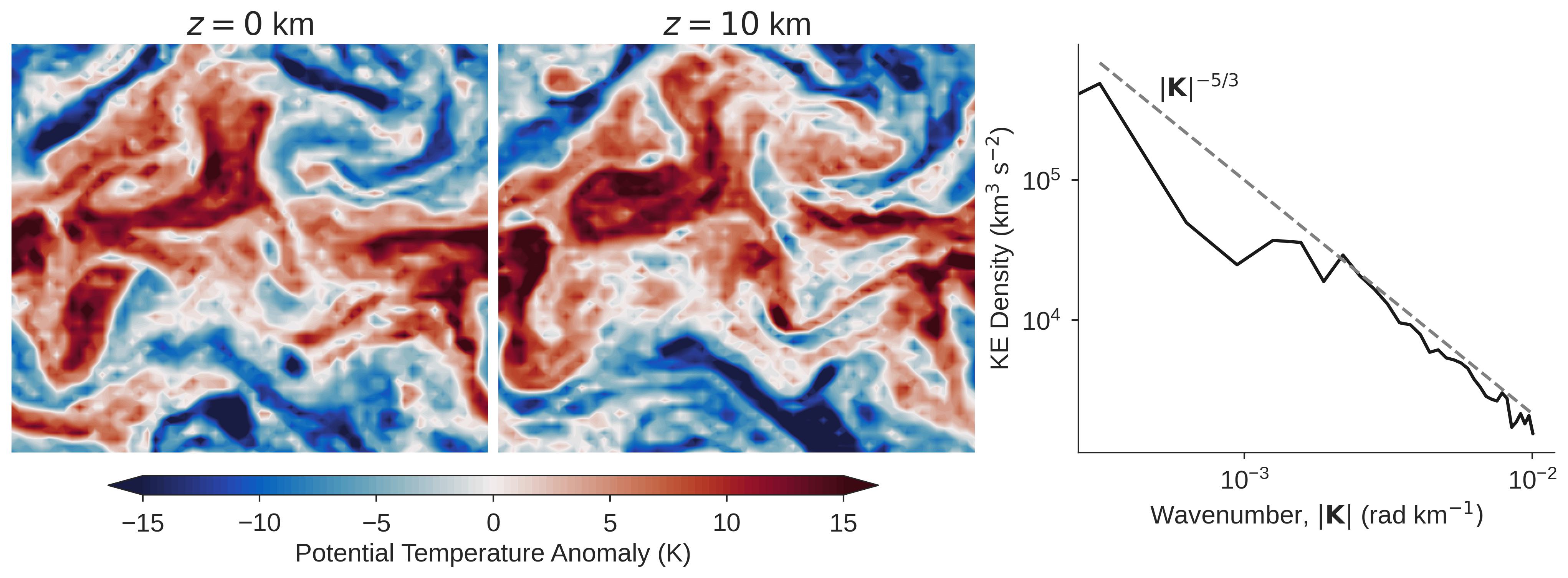
Our model configuration is discretized in space with and , uses a periodic boundary in both horizontal directions, and uses a timestep of minutes. To generate datasets for the neural networks, we initialize the model with Gaussian i.i.d. noise and spinup for 360 days, which we define as one model year. The spinup period is discarded, and we then generate a 25 year dataset that we partition into training (first 15 years), validation (next 5 years), and testing (final 5 years). For validation and testing, we randomly select 12 hour time windows from each respective dataset.
3 Single Layer Autoregressive and Recurrent Neural Networks
Our goal is to develop an emulator that can reproduce the time evolution of a chaotic dynamical system, such that its future state can be predicted from an initial state estimate. Therefore we use the following generic, discrete-time equations for our recurrent and autoregressive models,
| (1) | ||||
as by Goodfellow et al. (2016). Here denotes a particular timestep , where is the timestep size of the neural network, which may be larger than minutes, the step size of the original model described in Section 2. Here is the state of the dynamical system and is the hidden or internal state of the network, which is also referred to as the “reservoir” in RC or “feature vector” in NVAR. The generic function evolves this hidden state forward in time subject to the explicit influence of the current hidden and system states, as well as the macro-scale parameters . The output layer, , or “readout” operation, maps the hidden state back to the original state space, giving an approximation of the target system.
During the training phase, is provided to the model at each timestep and the misfit between the approximation and data, , is used to train the weights in the output layer. After training, during the prediction phase, the network becomes an autonomous system:
The neural network architectures that we use employ a common structure that is relevant to the readout operator and training procedure; we discuss these details in Section 3.1. Additionally, we employ a similar strategy to parallelize the architecture for high dimensional systems, and this is discussed in Section 3.2. Finally, the specific form of for the ESN and NVAR architectures is provided in Sections 3.4 and 3.3, respectively.
3.1 Linear Readout and Training
The neural networks that we use employ two simplifications relative to the generic form presented in Equation 1. First, any internal relationships encapsulated within are pre-defined by the macro-scale parameters, . Therefore, no internal weights contained within are learned during the formal training process. Secondly, the readout operator is linear, such that
where is a matrix. The result of these two assumptions is a cost function that is quadratic with respect to the elements of ,
| (2) |
Here is the Frobenius norm, is the number of time steps used for training, is a Tikhonov regularization parameter (Tikhonov (1963)), chosen to improve numerical stability and prevent overfitting.
The hidden and target states can be expressed in matrix form by concatenating
each time step “column-wise”:
,
and similarly
.
With this notation, the elements of can be compactly written as the
solution to the linear ridge regression problem
| (3) |
although we do not form the inverse explicitly. We instead use the solve function from SciPy’s linear algebra module (Virtanen et al. (2020)), based on testing shown in <Appendix C of¿[]platt_systematic_2022.
3.2 Parallelization Strategy
The model architectures that we use inherit the gridded structure of the target state being emulated, and often require hidden states that are to times larger than the target system dimension. Atmosphere and ocean GCMs typically propagate high dimensional state vectors, ranging from to , so representing the system with a single hidden state would be intractable. Thus, we employ a parallelization strategy to distribute the target and hidden states across many semi-independent networks. Our strategy follows the algorithm introduced by Pathak et al. (2018), and follows a similar construction as Arcomano et al. (2020). We outline the procedure here and note an illustration of the process for the ESN architecture in Figure 3.
We subdivide the domain into rectangular groups based on horizontal location, akin to typical domain decomposition techniques for atmosphere and ocean GCMs on structured grids. Each group contains horizontal grid cells, and all vertical grid cells at each horizontal location. The global state vector, , which consists of all state variables to be emulated at all grid cells, is partitioned into local state vectors, . For example, Figure 3 shows a field decomposed into nine groups, where each group is delineated by white lines. In our SQG predictions, we set , resulting in .
In order to facilitate interactions between nearby groups, each group has a designated overlap, or “halo”, region which consists of elements from its neighboring groups. The local group and overlapping points are illustrated in Figure 3 with a black box. The local state vectors, plus elements from the overlap region, are concatenated to form local input state vectors, . The result from the network is the local output state vector, , which is expanded to fill the target group as illustrated by the white box on the prediction shown in Figure 3. Here we set , so that and , given that and .
The local input vectors drive separate networks at each group, thereby generating distinct hidden states for each group as follows
| (4) | ||||
We make the assumption that the macro-scale parameters which determine internal connections within are globally fixed. Therefore, the only components that drive unique hidden states in each group are the local input vector and the local readout matrix, .
During the training phase, each group acts completely independently from one another. Therefore, the training process is embarrassingly parallel and allows us to scale the problem to arbitrarily large state vectors across a distributed computing system, subject to resource constraints. During the prediction phase, neighboring elements must be passed between groups in order to fill each overlap region at each time step with the most accurate state estimate possible, to ensure spatial consistency across the domain.
3.3 Nonlinear Vector Autoregression Design
Following Gauthier et al. (2021) and T-C. Chen et al. (2022), we consider forming the hidden state by using polynomial combinations of the time-lagged input state. We explain this process with a simple example using a two variable system, , a maximum polynomial degree , and a generic maximum number of lagged states :
| (5) | ||||
Clearly, the size of the hidden state vector grows rapidly with and , even for relatively low dimensional systems (<)see supplemental material of¿[for explicit calculations]chen_next_2022. We therefore make a simplification to the generic polynomial NVAR model. That is, we only represent nonlinear interactions between points that lie within a given radius between one another, defined by the number of neighboring points, . As a simple example, with and , the quadratic elements of a periodic, four variable system would be
ignoring “non-local” interactions such as . In order to make this parameter consistent with the overlap region in the parallelization scheme (Section 3.2), we set . Note, however, that we do model “non-local” linear interactions, up to the number of grid cells in each local group, i.e., containing points.
All of the remaining macro-scale parameters that determine the NVAR performance are
By using the preconditioning scheme introduced by T-C. Chen et al. (2022), we found results to be insensitive to the Tikhonov parameter , and so we fix this to . As noted earlier, we set . Our assumption behind this decision is that the NVAR model will be able to learn local quantities like gradients and fluxes between neighboring grid cells. Based on the results from T-C. Chen et al. (2022), the NVAR model should then be able to use this information to construct arbitrarily complex time stepping schemes as a function of . Because of its explicit nature, we manually vary to understand how memory impacts NVAR prediction skill.
3.4 Echo State Network Design

Our ESN architecture is illustrated in Figure 3, and is defined as follows
| (6) | ||||
Here is a leak parameter, is an adjacency matrix that determines the internal connections between the nodes of the hidden state, maps the input vector into the higher dimensional hidden state, and is the bias vector with elements . Unless otherwise specified, each ESN model uses a hidden layer width of . Finally, we note that ESNs require a spinup period before generating predictions, so we specify a 10 day spinup period for all validation and testing samples.
Two scalar parameters, and , are used to control the scaling of the adjacency and input matrices, respectively. These parameters have a dramatic influence on ESN prediction skill, since their values influence the network’s memory and stability (Lukoševičius (2012); Hermans & Schrauwen (2010)). Here we first normalize the matrices by their largest singular value, and then apply the scaling parameters as follows
where the elements of are initialized with elements . The initial adjacency matrix is generated similarly, except that the indices are randomly chosen such that attains a specified sparsity. Here we set the matrix sparsity to , with , following the success of very sparsely connected adjacency matrices as shown by Griffith et al. (2019). By first normalizing the matrices by the largest singular value, the parameters and re-scale the induced 2-norm of the matrix. This normalization is not standard in the ESN literature, but we found that it helped improve prediction skill. We provide further discussion of this process in Appendix A.
In summary, the macro-scale parameters that determine the overall characteristics of the ESN are
| (7) |
which are globally fixed for all groups. Due to the high sensitivity of ESN prediction skill to these parameter values, we follow the general optimization framework described by Platt et al. (2022) to determine approximately optimal values. We use the Bayesian Optimization algorithm outlined by Jones et al. (1998) and implemented by Bouhlel et al. (2019) to tune them. This process is discussed in Section 5. However, we first focus on prediction skill using the NVAR architecture in Section 4.
4 Nonlinear Vector Autoregression Prediction Skill
In this section we show the prediction skill of the polynomial based NVAR architecture described in Section 3.3. Note that we show the prediction skill of the ESN architecture in Section 5. To quantitatively evaluate each forecast, we compute the normalized root-mean-square error (NRMSE)
| (8) |
which is averaged over each spatial dimension, succinctly represented as a summation over , and normalized by the standard deviation, , computed from the true trajectory over time and all spatial dimensions. Additionally, we compute the relative error in terms of the kinetic energy (KE) density spectrum,
| (9) |
where and are the true and predicted KE density coefficients for each timestep and wavenumber , respectively (e.g., as in the right panel of Figure 2). Note that denotes the absolute value operation, and we retain the sign of the error in order to show a sense of the spectral error in each prediction.
We compute these quantities based on 50 twelve-hour predictions initialized from a random set of initial conditions taken from an unseen test dataset. To compactly visualize the skill over all samples, each lineplot in the following subsections shows a sample-average value with a solid line, and the 99% confidence interval with shading. We note that in some cases the model trajectory becomes unstable to the point that infinite values are produced. In the event that any single sample from a distribution has produced infinity, we take the more conservative approach and cut off any statistical averaging or confidence interval computation at that point in time and carry it no further. Therefore, some plots of NRMSE over time do not extend over the full 12 hour window, even though some sample trajectories are still valid, e.g., Figure 5 (left).
4.1 Temporal Subsampling


Figure 4 shows a qualitative comparison of NVAR predictions as a function of , i.e., how frequently the training data are sampled and the model makes predictions. For this figure, we set , and note that both the NRMSE and a snapshot of the KE density relative error corresponding to this configuration are shown in Figure 5.
At the model timestep ( min; ), the NVAR predictions are qualitatively similar to the truth for short forecast lead times. That is, the NRMSE is near 0, and many of the small scale features that exist in the truth are also evident in the predictions. However, at longer lead times the predictions become unstable. NRMSE spikes rapidly at about 4 hours after numerical instabilities are generated, which causes the NVAR model to produce physically unrealistic results. For reference, Figure S1 shows a view of what these numerical instabilities look like at their onset.
As the temporal resolution of the data is reduced, i.e., as increases, the predictions are generally stable for a longer period of time. Figure 5 shows that for , predictions are stable for roughly 6 hours, and for no predictions generate numerical instabilities over the 12 hour window. However, this stability comes with a cost: as the temporal resolution is reduced, the model’s representation of small scale features diminishes as these features become more blurry or smoothed. This blurring effect is apparent in Figure 4, where the prediction is qualitatively more blurry as increases in each panel from left to right.
This smoothing behavior is captured quantitatively in the right panel of Figure 5, which shows the KE relative error as in Equation 11. Here, we show the KE relative error after only 1.33 hours to show the behavior before instabilities dominate the predictions. The plot indicates the degree of spectral bias in each solution, which is largest at the smaller spatial scales, corresponding to higher wave numbers.
At there is a small positive bias at the smallest resolved spatial scales, indicating that this is when numerical instabilities are starting to generate. The subsampled runs, , show a negative bias, which corresponds to a dampened energy spectrum at the scales that are not resolved in the qualitatively smooth predictions shown in Figure 4. This negative bias is clearly larger with higher subsampling, or reduced temporal resolution, suggesting that as the data are subsampled, the network becomes incapable of tracking the small scale dynamics. The result is an averaged view of what may be occurring in between each time stamp.
4.2 Prediction Skill as a Function of Memory
A key feature of RNNs and autoregressive models is that they retain memory of previous system states. Given the explicit nature of the NVAR architecture, we explore the effect of adding memory by increasing , the number of lagged states used to create the feature vector. We first summarize how memory impacts prediction skill in Figure 6, which shows the NRMSE as a function of (colors) for each subsampling factor (panels). For any value of , adding memory (increasing ) reduces the short term error. However, adding memory also tends to increase error by the end of the forecast, often leading to the development of numerical instabilities and an incoherent solution. Similarly, for any fixed value of , increasing the temporal resolution (decreasing ) shows the same behavior.

To shed some light on how this additional memory impacts the solution, we show the KE relative error for the case of as a function of time (panels) and (colors) in Figure 7. For about the first 4 hours, increasing memory improves prediction skill at all spatial scales. However, beyond this point, the overall NRMSE grows rapidly, the improvement at small scales ( rad km-1) is more muted, and error is propagated rapidly into the larger spatial scales.
We surmise that adding memory degrades the long term prediction skill in the quadratic NVAR because the relationship between points further back in history are governed by higher order nonlinear interactions that are incorrectly represented by the simple local-quadratic relation that is used here. As more terms are added that are incorrectly represented, the model becomes more and more unstable. We make this supposition based on the fact that despite theoretical similarities between NVAR and ESNs as highlighted by Bollt (2021), we attain stable predictions using an ESN architecture with a hyperbolic tangent activation function in Section 5.
The question for the NVAR architecture is therefore how to retain the short term benefit of added memory capacity throughout the forecast horizon while maintaining a stable trajectory. While it may seem natural to explore higher order polynomials to properly represent this history, we do not explore this further because the size of the feature vector grows dramatically with the polynomial order (T-C. Chen et al. (2022)). Another option would be to explore entirely different basis functions. While this could be a potential option for future work, we note the findings of Zhang & Cornelius (2022), who show the extreme sensitivity of NVAR to the form of nonlinearity imposed. Given that it is an entirely open question on how to represent the smallest scales of geophysical turbulence, we do not explore other basis functions, and instead turn to the more general ESN architecture.
5 Echo State Network Prediction Skill
In this section we show the prediction skill of the more general ESN architecture outlined in Section 3.4. Here we use similar metrics as in Section 4 to evaluate the ESN skill, except that we show time averaged quantitative metrics because all of the ESN predictions are stable for the full twelve-hour forecast horizon. That is, when shown as a single distribution rather than a time series, NRMSE is reported as
| (10) |
where consists of the number of timesteps in the trajectory. In order to characterize spectral error, we show the KE relative error as in Section 4. Additionally, we show the NRMSE in terms of the KE density spectrum as follows
| (11) |
where is the number of spectral coefficients and is the temporal standard deviation of each spectral coefficient throughout the test trajectory. As in Section 4, all distributions and lineplots indicate prediction skill from 50 randomly selected initial conditions from an unseen test dataset.
5.1 Soft Constraints on Spectral Error
It is well known that ESN prediction skill is highly dependent on the global or “macro-scale” parameters noted in Equation 7, (<), e.g.¿[]platt_systematic_2022,lukosevicius_practical_2012. Following the success of previous studies in using Bayesian Optimization methods to systematically tune these parameters (Griffith et al. (2019); Penny et al. (2022); Platt et al. (2022)), we use the Bayesian Optimization algorithm outlined by Jones et al. (1998) and implemented by Bouhlel et al. (2019) to find optimal parameter values.
More recently, Platt et al. (2023) showed that constraining these macro-scale parameters using global invariant properties of the underlying system leads the optimization algorithm to select parameters that generalize well to unseen test data. In that work, the authors were successful in using the largest positive Lyapunov exponent, and to a lesser extent the fractal dimension of the system. Because of the focus on resolved scales in this work, we take a similar approach, but test the effect of constraining the ESN to the KE density spectral coefficients. Specifically, we implement the following two-stage training process. At each step, the macro-scale parameters, , are fixed, and the “micro-scale” parameters are obtained by minimizing Equation 2. This readout matrix is then used to make forecasts from randomly selected initial conditions from a validation dataset. The skill of each of these forecasts is captured by the macro-scale cost function
| (12) |
where NRMSE and KE_NRMSE are defined in Equations 10 and 11, is the number of forecasts used in the validation set, and is a hyperparameter that determines how much to penalize deviations from the true KE density spectrum. The value of is then used within the Bayesian Optimization algorithm, which reiterates the whole optimization process with new values for until an optimal value is found or the maximum number of iterations is reached. Here, we use , initialize the optimization with 20 randomly sampled points in the 5 dimensional parameter space, and run for 10 iterations. Note that we run this optimization procedure for each unique ESN configuration throughout Section 5 (i.e., for each and each value).
Figure 8 shows a qualitative view of how penalizing the KE density impacts ESN prediction skill when it operates at the original timestep of the SQG model (i.e., ). At , the ESN parameters are selected based on NRMSE alone, and the prediction is relatively blurry. However, as increases to , the prediction becomes sharper as the small scale features are better resolved.
Figure 9 gives a quantitative view of how the KE density penalty changes ESN prediction skill, once again with . The first two panels show that there is a clear tradeoff between NRMSE and KE error: as increases the NRMSE increases but the spectral representation improves. The final panel in Figure 9 shows that the spatial scales at which the spectral error manifests in these different solutions. When , the macro-scale parameters are chosen to minimize NRMSE, leading to blurry predictions and a dampened spectrum at the higher wavenumbers, especially for rad km-1. We note that Lam et al. (2022) report the same behavior when using a cost function that is purely based on mean-squared error. On the other hand, when , the global parameters are chosen to minimize both NRMSE and KE density error, where the latter treats all spatial scales equally. In this case, KE relative error is reduced by more than a factor of two and the spectral bias at higher wavenumbers is much more muted.
Of course, the tradeoff for the reduced spectral error is larger NRMSE, resulting from slight mismatches in the position of small scale features in the forecast. However, our purpose is to generate forecasts that are as representative of the training data as possible. Overly smoothed forecasts are not desirable, because this translates to losing local extreme values, which are of practical importance in weather and climate. Additionally, a key aspect of ensemble forecasting is that the truth remains a plausible member of the ensemble (Kalnay et al. (2006)). Therefore, representing the small scale processes, at least to some degree, will be critical for integrating an emulator into an ensemble based prediction system.
Finally, we note that using a cost function with only KE_NRMSE produced inconsistent results. Therefore, we consider it important to keep the NRMSE term in the cost function, as this prioritizes the position of small scale features, i.e., maintains phase information. Additionally, we note that there is some irreducible high wavenumber error, which is most clearly seen by comparing the prediction skill to a persistent forecast. While the sample median NRMSE for each value beats persistence, the KE_NRMSE is more than double, due to this error at the small spatial scales. Ideally, our forecasts would beat persistence in both of these metrics, but obtaining the “realism” in the small spatial scales necessary to dramatically reduce this spectral error should be addressed in future work.

5.2 Temporal Subsampling
The NVAR predictions shown in Section 4.1 indicate that subsampling the training data systematically increases error at small spatial scales. However, the architecture was not specifically designed or constrained to have a good spectral representation of the underlying dynamics. On the other hand, the previous section (Section 5.1) showed that the spectral bias at high wavenumbers can be reduced by optimizing the global ESN parameters to the true KE density spectrum. Given these two results, we explore the following question: does temporal subsampling still increase spectral bias in the more general ESN framework, even when parameters are chosen to minimize this bias?
Figure 10 and Figure 11 show that even when the macro-scale parameters are chosen to prioritize the KE density representation (i.e., is fixed), temporal subsampling does lead to an apparently inescapable spectral bias. This effect is shown qualitatively in Figure 10, where the predictions become smoother as the temporal subsampling factor, , increases. The effect is similar to what was seen with NVAR except the blurring effect is less pronounced. Quantitatively, Figure 11(b) shows that as increases, error in KE density spectrum generally increases, while panel (c) shows that this KE error is concentrated in the small spatial scales, rad km-1. We note that the degree of spectral bias at is smaller than what was achieved with NVAR for the same value, cf. Figure 7, indicating that the optimization was successful in reducing the spectral bias.

Interestingly, there is little difference between NRMSE obtained by the ESNs at different values. Additionally, Figure 12 shows that there is little difference in both NRMSE and KE_NRMSE when , i.e., when NRMSE is the only criterion for parameter selection. This result shows that NRMSE alone is not a good criterion for model selection, given that we have shown success in reducing spectral errors by prioritizing the spectrum appropriately.
5.3 Impact of the Hidden Layer Dimension
The dimension of the hidden layer, , also known as the reservoir size, determines the memory capacity available to the ESN (Jaeger (2001); Lukoševičius (2012)). For systems with high dimensional input signals, it is crucial to use a sufficiently large hidden layer to afford the memory capacity necessary for accurate predictions (Hermans & Schrauwen (2010)). In all of the preceding sections we fixed for each local group, where for reference each local group has an input dimension of and an output dimension of . Here, we briefly address the effect of doubling the hidden layer dimension, while keeping the input and output dimensions constant, in order to test how sensitive our conclusions are on this crucial hyperparameter. Due to the computational expense of the parameter optimization discussed in Section 5.1, we only perform this experiment for .
The impact of doubling on prediction skill is shown in Figure 13, where for the sake of brevity we only show results for the case when in Equation 12. The left panel shows that the larger hidden layer actually increases the NRMSE slightly. However, the middle and right panels show that this increase is due to the improved spectral representation. The improvement in KE_NRMSE is nearly proportional to the improvement achieved by increasing the temporal resolution of the data. That is, doubling the hidden layer width reduces the average KE_NRMSE by 14%, while increasing the temporal resolution of the data by a factor of 4 reduces the KE_NRMSE by 30%. These results indicate a potential brute force approach to overcoming the subsampling related spectral errors. However, the larger hidden layer dimension has to be constrained with enough training data, and requires more computational resources.
5.4 Impact of Training Dataset Size
In all of the preceding experiments, the length of training time was fixed to 15 years, meaning that there are fewer training samples when the data are subsampled, i.e., as grows. Specifically, 15 years of data at an original model timestep of 5 minutes means that there are approximately , , and samples for each case previously shown: , 4, and 16, respectively. Here, we show that even when the number of training samples is fixed, the subsampling related spectral errors are still present.
Figure 14 shows the prediction skill in terms of NRMSE and spectral errors when the number of training samples is fixed to . With this number of samples, the training data is exactly the same for , but only spans and years for and , respectively. However, we see the same general trend as before: subsampling the data improves NRMSE slightly but increases the KE_NRMSE. As before, the spectral error is largest in the higher wavenumbers, rad km-1. We note that the difference in performance between and is marginal. The only notable difference between these two cases is that the ESN is less consistent, i.e., the KE_NRMSE distribution is broader, when . However, it is clear that spectral error is lowest when the data are not subsampled at all, even though less than a year of data is used. This result indicates that there could be a benefit to training a RNN on a relatively shorter model trajectory that is untouched, rather than a longer dataset that is subsampled in time.
6 Discussion
Weather and climate forecasting necessitates the integration of expensive numerical models to make accurate predictions and projections. The computational cost of these models often results in tradeoffs, where practitioners must balance the spatial resolution of their model with other factors, such as the number of integrated model components or the ensemble size that can be afforded in the system. Model emulation or surrogate modeling aims to enable such predictions by emulating the dynamical system with adequate accuracy at a much lower computational expense. In this study, our primary interest was to shed light on the spatial scales that can be resolved by single layer autoregressive and recurrent neural network emulators in order to better understand the effective resolution that could be achieved in weather and climate applications. We used two relatively simple, single layer autoregressive and recurrent neural network architectures, mainly because it has been shown that they can successfully emulate low dimensional chaotic dynamics over multiple Lyapunov timescales (Pathak et al. (2017); Vlachas et al. (2020); Gauthier et al. (2021); Platt et al. (2022)). We implemented a multi-dimensional parallelization scheme based on the concept introduced by Pathak et al. (2018) and similar to that of Arcomano et al. (2020) in order to scale up these architectures and test them in high dimensional systems. We note that an in-depth discussion of our software implementation using the task based scheduling system in python, Dask (Dask Development Team (2016)), will be covered in a forthcoming paper.
6.1 Main Result and Connections to Previous Work
Our main result is that we observe an inherent spectral bias that occurs when training data are subsampled in time, such that as the temporal resolution is reduced, the resolution of small scale features in NVAR and ESN predictions is diminished. High wavenumber spectral bias is a phenomenon that has been studied in the context of training feed forward neural networks (<)see¿[for a comprehensive review on the topic]xu_overview_2022. The authors show that while numerical Partial Differential Equation (PDE) solvers typically resolve small spatial scales first and iteratively refine the larger spatial scales, spectral biases arise while training neural networks because the reverse happens: the large scales are uncovered first and small spatial scales are slowly refined.
Here, we showed a similar bias that arises in NVAR and ESN architectures in relation to their temporal resolution. Given the sensitivity to model time step, this phenomenon bears resemblance to the Courant-Friedrich-Lewy (CFL) condition, which poses an upper bound on the time step size that can be used in the numerical solution of PDEs. The CFL condition is therefore a barrier to weather and climate model efficiency. However, sensitivity to the time step size manifests very differently in neural networks and numerical PDEs. While violating the CFL condition with too large of a time step leads to fundamental issues of numerical instability in numerical PDEs, here we see that increasing the time step adds a sort of numerical dissipation, which can actually stabilize an otherwise unstable model architecture (Section 4.1). We suggest that this occurs because the small scales are “lost” within the recurrent and autoregressive time stepping relations. Because of this, the models are trained to take on an interpolated or spatially averaged view of the intermediate dynamical behavior, which generates a blurred prediction.
We note that Bi et al. (2022) discuss a similar phenomenon relating to the timestepping of their autoregressive transformer model. Specifically, they devise a “Hierarchical Temporal Aggregation” scheme to make more stable and accurate forecasts (in terms of RMSE) over longer periods of time than they would potentially be able to if they were to use the original 1 hour cadence of the ERA5 dataset. However, it is not clear how well small scale features are preserved with this approach. This is unclear first because they use a cost function that is purely based on RMSE. Secondly, the approach requires training multiple models at successively larger time intervals, and a forecast is made using the largest interval possibly available first. For instance, with trained models operating on 1 and 6 hourly increments, a 7 hour forecast would be made by first a 6 and then 1 hour prediction. Our results indicate that this could be problematic, as the model making the 6 hour prediction would filter out small scale features that would otherwise be captured by the second model, operating on a 1 hour timestep.
Finally, Chattopadhyay & Hassanzadeh (2023) show the connection between high wavenumber spectral bias and instabilities in neural network predictions of turbulent flows. Their focus was on achieving long term stability in neural network time stepping for climate applications, while the focus in our work has been on short term forecasting for weather applications - capturing the long term, climate statistics in turbulent geophysical fluid dynamics with an ESN or NVAR is future work. However, both works (1) draw some connection between high frequency spectral bias and the time stepping of the neural network, and (2) offer potential solutions by penalizing the solution’s spectrum. In our work, we show that some of the spectral bias stems from the timestep size of the data used for training, while Chattopadhyay & Hassanzadeh (2023) devise a Runge-Kutta scheme to reduce the bias on subsampled data. Additionally, they use a spectral loss to train the internal weights of the network, along with the addition of a “corrector” network to make predictions of only the small scales. On the other hand, we use a spectral loss to guide the optimization of 5 “macro-scale” parameters, but the training of the network weights and operation of the network remain the same. Despite the differences in approach, the similarity of these two works indicates that the details of neural network time stepping schemes are crucial to their stability and accuracy in representing small scale processes. Additionally, it is clear that these small scale processes must be prioritized in some way, for instance through a loss function, and potentially additional “corrector” networks that propagate the small scales explicitly.
6.2 Implications for Training Datasets in Weather and Climate
This result has important implications for the rapidly developing field of neural network emulation for weather and climate forecasting because it shows a potential limit to the effective resolution of an emulator relative to the original training data. If an emulator is used as a parameterization scheme for subgrid-scale dynamics, then a high wavenumber spectral bias will be detrimental to performance. Additionally, we surmise that such errors will reduce ensemble spread within data assimilation algorithms, which could limit their usefulness within a forecasting system (<)e.g.,¿[]kalnay_ensemble_2006. Our findings are pertinent to the field of neural network emulation development because of the widespread usage of reanalysis datasets for training. Currently, most existing neural network emulators in this field use the ERA5 reanalysis dataset (Hersbach et al. (2020)) for training (<)e.g.,¿[]lam_graphcast_2022,bi_accurate_2023,pathak_fourcastnet_2022,keisler_forecasting_2022,weyn_sub-seasonal_2021,arcomano_machine_2020. Of course, reanalyses like ERA5 are an obvious choice for many reasons: the datasets are made freely available, they present a multi-decadal view of weather and climate, and, most importantly, they are constrained to observational data. However, we note that reanalysis products are imperfect for at least the following reasons: they contain jumps in the system state at the start of each DA cycle, they may contain inconsistencies reflective of changes in observational coverage, and they are only made available at large time intervals relative to the time step of the underlying integrated numerical model dynamics, due to the massive size of the data. Our study only addressed the latter of these issues, and showed that this simple space-saving step can have a negative impact on data-driven prediction methods. While we showed that adding spectral error as a weak constraint in the neural network training can reduce this time step related spectral bias, our results indicate that the underlying issue persists (Section 5.2). Moreover, as long as the data are not subsampled, we showed that ESNs perform only slightly worse when year of data are used, compared to 15 years of training data (Section 5.4). This result suggests that it may be more effective to design an RNN-based emulator with a relatively short model trajectory that is not subsampled, rather than a long trajectory that is subsampled. In contrast to training the emulator on a reanalysis dataset, a pure model-based emulator could then be used within a data assimilation system as by Penny et al. (2022) in order to additionally benefit from observational constraints.
6.3 Implications and Future Work Relating to Model Architecture
Due to the fact that RNNs require long, sequential data streams in order to learn the governing dynamics, it could be the case that RNNs suffer most dramatically from temporal subsampling. This hypothesis could be one reason for why the RNNs used by Agarwal et al. (2021) performed worse than other models on data that were subsampled every 10 days. Additionally, if RNNs are most dramatically affected by temporal subsampling, then they could be a suboptimal architecture choice for model emulators in cases where representing small scale dynamics is important but a coarse time step is required. This requirement is especially true when designing a parameterization scheme for subgrid-scale dynamics, where the emulator should ideally run at the same time step as the “large-scale” model.
However, given that we can qualitatively observe some degree of spectral error in a wide variety of neural network architectures that use subsampled data for training (<)e.g.,¿[]lam_graphcast_2022,bi_accurate_2023,pathak_fourcastnet_2022,keisler_forecasting_2022, the issue could be more general to other neural network architectures. Moreover, the similarities between our work and Chattopadhyay & Hassanzadeh (2023) as well as the reasons behind the hierarchical time stepping scheme introduced by Bi et al. (2022) (both discussed in Section 6.1) imply that the time stepping related spectral bias is a general issue. Therefore, we suggest that future work should be directed at understanding the degree to which temporal resolution affects architectures other than RNNs. Potential avenues could include exploring how attention mechanisms (Vaswani et al. (2017); Dosovitskiy et al. (2021)) handle this phenomenon. Additionally, in light of our results indicating that wider networks can mitigate the spectral bias at least to some degree (Section 5.3), it would be instructive to understand how successively adding layers to a neural network affects the spectral bias. Finally, we note the work of Duncan et al. (2022) who show success in using adversarial training to mitigate the spectral bias observed in FourCastNet, and suggest that such techniques deserve additional study to understand their robustness.
Of course, our neural network implementations are imperfect, and we suggest some future avenues to improve their predictive capabilities. Both of the architectures relied on a mean-squared error micro-scale cost function to learn the readout matrix weights, even in the ESN models where the spectral errors were penalized in the macro-scale cost function. However, even when the spectrum was penalized and the data were not subsampled, the ESNs maintained a high wavenumber bias that resulted in KE_NRMSE far greater than that of a persistent forecast. While additional testing shows that a periodic sine activation function can reduce the high frequency bias in KE_NRMSE, following work by Sitzmann et al. (2020), the underlying problem still remains (see additional analysis in the Supplemental Materials). Therefore, in order to further reduce the high frequency bias, it may be necessary to move the spectral penalties to the micro-scale cost function, i.e., to learn the readout matrix weights in the case of reservoir computing. The time stepping, spectral loss, and “small scale corrector network” employed by Chattopadhyay & Hassanzadeh (2023) would be appropriate starting points for such future work.
The NVAR architecture that we employed is incredibly simple. While we supposed that the local quadratic feature vector could learn quantities like derivatives and fluxes necessary to step the model forward in time, it is apparently not robust enough given the dramatic sensitivity to time step used. Future work could explore the possibility of using a larger library of analytic functions to improve the nonlinear expressions in the model, with the caution that this will lead to very high dimensional feature vectors. Such developments must sufficiently address the “Catch-22” described by Zhang & Cornelius (2022), who show that NVAR is inherently sensitive to the types of nonlinearity chosen. It is entirely possible, though, that an appropriate set of such basis functions exist for weather and climate emulation.
The ESN architecture that we employed is also relatively straightforward, and can undoubtedly be improved. In this work we took a somewhat brute force approach to emulate arbitrarily high dimensional systems by partitioning the system into subdomains and deploying parallel ESNs on each group. However, this process comes with overhead and can still lead to rather large networks on each group. The memory costs associated with these large networks coupled with any additional computational costs associated with timestepping, either by increasing the frequency or by using a more expensive method to represent small scale processes, will likely make the ESN implementation shown here too expensive to be considered for practical applications. Future work could explore dimension reduction techniques involving proper orthogonal decomposition (Jordanou et al. (2022)), autoencoders (Heyder et al. (2022)), or approaches involving self-organizing or scale invariant maps (Basterrech et al. (2011)). Similarly, Whiteaker & Gerstoft (2022) show success in deriving a controllability matrix for the ESN, which leads to a reduced network size with minimal reduction in error. Finally, a number of studies claim to have developed ESN architectures that can capture dynamics occurring at many scales (Moon et al. (2021); Ma et al. (2020); Gallicchio et al. (2018); Gallicchio et al. (2017); Malik et al. (2017)), and these could be explored for geophysical turbulence emulation as well.
7 Conclusions
Recent advances in neural network based emulators of Earth’s weather and climate indicate that forecasting centers could benefit greatly from incorporating neural networks into their future prediction systems. However, a common issue with these data-driven models is that they produce relatively blurry predictions, and misrepresent the small spatial scale features that can be resolved in traditional, physics-based forecasting models. Here, we showed that the simple space saving step of subsampling the training data used to generate recurrent neural network emulators accentuates this small scale error. While we show some success in mitigating the effects of this subsampling related, high wavenumber bias through an inner/outer loop optimization framework, the problem persists. Many neural network emulators use subsampled datasets for training, including most prominently the ERA5 Reanalysis. While our work suggests that there could be a benefit to using a training dataset based on a relatively shorter model trajectory that is not subsampled, rather than a longer one that is, addressing the subsampling issue would provide more confidence in using already existing, freely available datasets like reanalyses. We therefore suggest that future work should focus on how other architectures and techniques like attention or adversarial training can address this subsampling related bias at the small spatial scales of turbulent geophysical fluid dynamics.
Appendix A Matrix and Data Normalization for Echo State Networks
Here we describe several aspects of our ESN implementation that are unique with respect to previous works. Additionally, we provide some empirical justification for these choices, using the Lorenz96 model as a testbed (Lorenz (1996)), see Appendix Section A.4 for a description of the datasets generated for these tests.
Our testing framework follows the general procedure laid out by Platt et al. (2022) to evaluate the architecture choices. For each design choice, we compute the Valid Prediction Time (VPT) of an ESN model over 100 randomly chosen initial conditions from a test dataset. VPT is computed as
where is a time index, is the temporal standard deviation of the -th dimension, computed from the training data, and . To eliminate the dependence of the results on the randomly chosen adjacency and input matrices, we repeat the process for 10 different adjacency and input matrix pairs, initialized with different random number generator seeds. In total, we compare each design choice with a VPT distribution from 1,000 test samples. We note that we optimize the ESN parameters listed in Equation 7 for each design choice and each random matrix pair, following the procedure described in Section 5.1 with an NRMSE cost function. Of course, these tests are insufficient to definitively prove that these choices will translate perfectly to the SQG system. However, we consider this to be a bare minimum test that will catch downright bad design choices, while saving the computing resources necessary to train an emulator for larger problems.
A.1 Input Matrix Scaling
Typically, is filled with entries
where determines the bounds of the uniform distribution. Here we found it to be advantageous to normalize the input matrix by the largest singular value. That is, we first compute , with elements
Then, we set as
where is the largest singular value, and the parameter is the desired largest singular value of .
Our motivation for using this type of normalization is that we found it necessary to use very wide parameter optimization bounds for when using the standard input scaling strategy. Normalizing the matrix by the largest singular value compensates for the fact that the amplitude of the contributions to the reservoir, i.e., the elements of the vector
grow with . By controlling for this growth, we were able to reduce the optimization search space and achieve more consistent prediction skill with fewer iterations.
Additionally, we found empirical evidence to suggest that this normalization is advantageous even for small systems. Figure 15 shows the VPT achieved with the 20-Dimensional Lorenz96 system (Appendix Section A.4), using a variety of normalization strategies for the input and adjacency matrices. In Figure 15, the two schemes used for the input matrix are (1) no normalization (indicated by ) and (2) normalization by the largest singular value (indicated by ). For a variety of reservoir sizes, , we found that using the largest singular value often performed better, usually by about 0.5 MTU.
A.2 Adjacency Matrix Scaling
Typically, the reservoir adjacency matrix is normalized to achieve a desired spectral radius. That is, the matrix is generated with elements , where are random indices in order to satisfy the desired sparsity of the matrix (all other elements are 0). Then, is set as
where is the spectral radius, and scales the matrix to achieve the desired spectral radius. A common guideline is to set , as it is hypothesized that this puts the reservoir on the “edge of stability” so that it performs well in emulating nonlinear systems (<)e.g., as recommended by¿[]lukosevicius_practical_2012. However, as originally described by Jaeger (2001), the spectral radius provides only a necessary, but insufficient, means to satisfy the required Echo State Property. On the other hand, using the largest singular value is a sufficient condition for satisfying the echo state property.
In our experimentation, we have found a slight benefit from using the largest singular value to normalize the adjacency matrix. Figure 15 shows that, for fixed input matrix normalization, using the largest singular value rather than spectral radius achieves similar and up to longer valid predictions. While the improvement may seem subtle, we note that using the largest singular value has the following practical benefit for our python-based implementation: the singular values can be computed directly on a Graphical Processing Unit using CuPy (Okuta et al. (2017)), while a general, non-symmetric eigenvalue decomposition is not readily available.
A.3 Data Normalization
A key aspect in machine learning is normalizing input data before passing it to the model. Experiments from Platt et al. (2022) showed, however, that the standard approach to normalizing data can be detrimental to prediction skill. By “standard approach”, we mean
where
i.e., and are the mean and standard deviation taken from the training data separately over each channel of data, indexed by . The key takeaway from Platt et al. (2022) is that by using separate normalization values for each channel, the covarying relationships between the data are destroyed and the reservoir cannot learn the true dynamics. The authors propose to normalize with the average and range of the data, computed over the length of the training data and over all channels
| (13) |
where
| (14) |
Here, we propose to replace the range in the denominator with the standard deviation computed over all channels and timesteps in the training data,
| (15) |
with
Figure 16 compares the prediction skill when these two normalization strategies are used. Using the standard deviation normalization as in Equation 15 leads to an average VPT increase of 2 MTU. We suggest that this improvement is due to the fact that when the data are normalized by the full range, then all values are in the range . In this case, once the input is mapped into the hidden space, it is more likely to lie on the linear regime of the activation function. While a large enough input scaling could eliminate this problem, it is apparently not easily obtained during the Bayesian optimization.
A.4 Lorenz96 Datasets
The Lorenz96 dataset used for these supplemental experiments were generated by the following set of equations introduced by Lorenz (1996),
where , and the domain is periodic. is a fixed parameter that generates chaotic dynamics. We use for the tests in Appendices Sections A.1 and A.2 and for the tests in Appendix Section A.3. Each dataset was generated by stepping the model forward with a 4th order Runge-Kutta scheme with Model Time Units (MTU). Each dataset consisted of a 10 MTU spinup period that was discarded, 420 MTU of training data, a 60 MTU validation period, and a 120 MTU test period. Each randomly chosen validation and test trajectory were 1 MTU and 15 MTU, respectively, and the ESN spinup period was 5 MTU.
Appendix B Gulf of Mexico Dataset and ESN Prediction
The Gulf of Mexico reanalysis dataset used to generate the prediction in Figure 1 was provided by HYCOM (2016). The data consists of 6 hourly snapshots of 2D sea surface height and 3D temperature, salinity, and zonal and meridional velocities, covering 1993-2012 (inclusive). We used only the top level of temperature, and used the first 18 years as training, and the last two years as test data. Here we apply a parallelized ESN architecture, using , , and . Because we use only the top level of temperature, , and therefore , . The grid cells that represent continental land are ignored in the input and output vectors, and in the corresponding rows of . Therefore, the effect of the boundary conditions on the neighboring grid cells is implicitly learned from the data.
Open Research
The model configurations used to generate the results in this manuscript can be found at Smith (2023).
Acknowledgements.
T.A. Smith and S.G. Penny acknowledge support from NOAA grant NA20OAR4600277. S.G. Penny and J.A. Platt acknowledge support from the Office of Naval Research (ONR) grants N00014-19-1-2522 and N00014-20-1-2580. T.A. Smith thanks Nora Loose for comments and discussion that improved the manuscript. The authors thank three anonymous reviewers and the handling editor for comments that improved the manuscript.References
- Agarwal et al. ((2021)) Agarwal, N., Kondrashov, D., Dueben, P., Ryzhov, E. & Berloff, P. (2021). A Comparison of Data-Driven Approaches to Build Low-Dimensional Ocean Models. Journal of Advances in Modeling Earth Systems 13 9 e2021MS002537. [2021-12-01]http://onlinelibrary.wiley.com/doi/abs/10.1029/2021MS002537 _eprint: https://agupubs.onlinelibrary.wiley.com/doi/pdf/10.1029/2021MS002537 doi:10.1029/2021MS002537
- Arcomano et al. ((2020)) Arcomano, T., Szunyogh, I., Pathak, J., Wikner, A., Hunt, B.R. & Ott, E. (2020). A Machine Learning-Based Global Atmospheric Forecast Model. Geophysical Research Letters 47 9 e2020GL087776. [2020-05-14]http://agupubs.onlinelibrary.wiley.com/doi/abs/10.1029/2020GL087776 _eprint: https://onlinelibrary.wiley.com/doi/pdf/10.1029/2020GL087776 doi:10.1029/2020GL087776
- Barbosa & Gauthier ((2022)) Barbosa, W.A.S. & Gauthier, D.J. (2022). Learning Spatiotemporal Chaos Using Next-Generation Reservoir Computing. arXiv:2203.13294 [nlin] . [2022-04-04]http://arxiv.org/abs/2203.13294 arXiv: 2203.13294
- Basterrech et al. ((2011)) Basterrech, S., Fyfe, C. & Rubino, G. (2011). Self-Organizing Maps and Scale-Invariant Maps in Echo State Networks. In 2011 11th International Conference on Intelligent Systems Design and Applications ( 94–99). ISSN: 2164-7151 doi:10.1109/ISDA.2011.6121637
- Bi et al. ((2022)) Bi, K., Xie, L., Zhang, H., Chen, X., Gu, X. & Tian, Q. (2022). Pangu-Weather: A 3D High-Resolution Model for Fast and Accurate Global Weather Forecast. : arXiv. [2022-11-23]http://arxiv.org/abs/2211.02556 arXiv:2211.02556 [physics]
- Bi et al. ((2023)) Bi, K., Xie, L., Zhang, H., Chen, X., Gu, X. & Tian, Q. (2023). Accurate medium-range global weather forecasting with 3D neural networks. Nature 619 7970 533–538. [2023-09-14]https://www.nature.com/articles/s41586-023-06185-3 Number: 7970 Publisher: Nature Publishing Group doi:10.1038/s41586-023-06185-3
- Blumen ((1978)) Blumen, W. (19781). Uniform Potential Vorticity Flow: Part I. Theory of Wave Interactions and Two-Dimensional Turbulence. Journal of the Atmospheric Sciences 35 5 774–783. [2021-11-24]https://journals.ametsoc.org/view/journals/atsc/35/5/1520-0469_1978_035_0774_upvfpi_2_0_co_2.xml Publisher: American Meteorological Society Section: Journal of the Atmospheric Sciences doi:10.1175/1520-0469(1978)035¡0774:UPVFPI¿2.0.CO;2
- Blumen ((1978)) Blumen, W. (19782). Uniform Potential Vorticity Flow: Part II. A Model of Wave Interacions. Journal of the Atmospheric Sciences 35 5 784–789. [2022-12-08]https://journals.ametsoc.org/view/journals/atsc/35/5/1520-0469_1978_035_0784_upvfpi_2_0_co_2.xml Publisher: American Meteorological Society Section: Journal of the Atmospheric Sciences doi:10.1175/1520-0469(1978)035¡0784:UPVFPI¿2.0.CO;2
- Bollt ((2021)) Bollt, E. (2021). On explaining the surprising success of reservoir computing forecaster of chaos? The universal machine learning dynamical system with contrast to VAR and DMD. Chaos: An Interdisciplinary Journal of Nonlinear Science 31 1 013108. [2021-11-03]https://aip-scitation-org.colorado.idm.oclc.org/doi/10.1063/5.0024890 Publisher: American Institute of Physics doi:10.1063/5.0024890
- Bouhlel et al. ((2020)) Bouhlel, M.A., He, S. & Martins, J.R.R.A. (2020). Scalable gradient–enhanced artificial neural networks for airfoil shape design in the subsonic and transonic regimes. Structural and Multidisciplinary Optimization 61 4 1363–1376. [2023-04-03]https://doi.org/10.1007/s00158-020-02488-5 doi:10.1007/s00158-020-02488-5
- Bouhlel et al. ((2019)) Bouhlel, M.A., Hwang, J.T., Bartoli, N., Lafage, R., Morlier, J. & Martins, J.R.R.A. (2019). A Python surrogate modeling framework with derivatives. Advances in Engineering Software 135 102662. [2023-02-11]https://www.sciencedirect.com/science/article/pii/S0965997818309360 doi:10.1016/j.advengsoft.2019.03.005
- Chattopadhyay & Hassanzadeh ((2023)) Chattopadhyay, A. & Hassanzadeh, P. (2023). Long-term instabilities of deep learning-based digital twins of the climate system: The cause and a solution. : arXiv. [2023-04-26]http://arxiv.org/abs/2304.07029 arXiv:2304.07029 [physics]
- T-C. Chen et al. ((2022)) Chen, T-C., Penny, S.G., Smith, T.A. & Platt, J.A. (2022). ‘Next Generation’ Reservoir Computing: an Empirical Data-Driven Expression of Dynamical Equations in Time-Stepping Form. : arXiv. [2022-12-05]http://arxiv.org/abs/2201.05193 arXiv:2201.05193 [cs, math] doi:10.48550/arXiv.2201.05193
- X. Chen et al. ((2021)) Chen, X., Nadiga, B.T. & Timofeyev, I. (2021). Predicting Shallow Water Dynamics using Echo-State Networks with Transfer Learning. arXiv:2112.09182 [physics] . [2022-01-11]http://arxiv.org/abs/2112.09182 arXiv: 2112.09182
- Cressie ((1993)) Cressie, N. (1993). Statistics for spatial data.
- Dask Development Team ((2016)) Dask Development Team. (2016). Dask: Library for dynamic task scheduling [ https://dask.org
- Dosovitskiy et al. ((2021)) Dosovitskiy, A., Beyer, L., Kolesnikov, A., Weissenborn, D., Zhai, X., Unterthiner, T.Houlsby, N. (2021). An Image is Worth 16x16 Words: Transformers for Image Recognition at Scale. : arXiv. [2022-11-23]http://arxiv.org/abs/2010.11929 arXiv:2010.11929 [cs]
- Dueben & Bauer ((2018)) Dueben, P.D. & Bauer, P. (2018). Challenges and design choices for global weather and climate models based on machine learning. Geoscientific Model Development 11 10 3999–4009. [2021-02-09]https://gmd.copernicus.org/articles/11/3999/2018/ Publisher: Copernicus GmbH doi:https://doi.org/10.5194/gmd-11-3999-2018
- Duncan et al. ((2022)) Duncan, J., Subramanian, S. & Harrington, P. (2022). Generative Modeling of High-resolution Global Precipitation Forecasts. : arXiv. [2023-01-06]http://arxiv.org/abs/2210.12504 arXiv:2210.12504 [physics] doi:10.48550/arXiv.2210.12504
- Eady ((1949)) Eady, E.T. (1949). Long Waves and Cyclone Waves. Tellus 1 3 33–52. [2023-01-04]https://onlinelibrary.wiley.com/doi/abs/10.1111/j.2153-3490.1949.tb01265.x _eprint: https://onlinelibrary.wiley.com/doi/pdf/10.1111/j.2153-3490.1949.tb01265.x doi:10.1111/j.2153-3490.1949.tb01265.x
- Evensen et al. ((2022)) Evensen, G., Vossepoel, F.C. & van Leeuwen, P.J. (2022). Data Assimilation Fundamentals: A Unified Formulation of the State and Parameter Estimation Problem. Cham: Springer International Publishing. [2022-06-08]https://link.springer.com/10.1007/978-3-030-96709-3 doi:10.1007/978-3-030-96709-3
- Gallicchio et al. ((2017)) Gallicchio, C., Micheli, A. & Pedrelli, L. (2017). Deep reservoir computing: A critical experimental analysis. Neurocomputing 268 87–99. [2023-03-30]https://www.sciencedirect.com/science/article/pii/S0925231217307567 doi:10.1016/j.neucom.2016.12.089
- Gallicchio et al. ((2018)) Gallicchio, C., Micheli, A. & Pedrelli, L. (2018). Design of deep echo state networks. Neural Networks 108 33–47. [2023-03-30]https://www.sciencedirect.com/science/article/pii/S0893608018302223 doi:10.1016/j.neunet.2018.08.002
- Gauthier et al. ((2021)) Gauthier, D.J., Bollt, E., Griffith, A. & Barbosa, W.A.S. (2021). Next generation reservoir computing. Nature Communications 12 1 5564. [2021-10-21]https://www.nature.com/articles/s41467-021-25801-2 Bandiera_abtest: a Cc_license_type: cc_by Cg_type: Nature Research Journals Number: 1 Primary_atype: Research Publisher: Nature Publishing Group Subject_term: Computational science;Electrical and electronic engineering Subject_term_id: computational-science;electrical-and-electronic-engineering doi:10.1038/s41467-021-25801-2
- Goodfellow et al. ((2016)) Goodfellow, I., Yoshua, B. & Aaron, C. (2016). Sequence Modeling: Recurrent and Recursive Nets. In Deep Learning. : MIT Press. https://www.deeplearningbook.org/
- Griffith et al. ((2019)) Griffith, A., Pomerance, A. & Gauthier, D.J. (2019). Forecasting chaotic systems with very low connectivity reservoir computers. Chaos: An Interdisciplinary Journal of Nonlinear Science 29 12 123108. [2021-11-29]https://aip.scitation.org/doi/10.1063/1.5120710 Publisher: American Institute of Physics doi:10.1063/1.5120710
- Hasselmann ((1988)) Hasselmann, K. (1988). PIPs and POPs: The reduction of complex dynamical systems using principal interaction and oscillation patterns. Journal of Geophysical Research: Atmospheres 93 D9 11015–11021. [2022-10-11]https://onlinelibrary.wiley.com/doi/abs/10.1029/JD093iD09p11015 _eprint: https://onlinelibrary.wiley.com/doi/pdf/10.1029/JD093iD09p11015 doi:10.1029/JD093iD09p11015
- Held et al. ((1995)) Held, I.M., Pierrehumbert, R.T., Garner, S.T. & Swanson, K.L. (1995). Surface quasi-geostrophic dynamics. Journal of Fluid Mechanics 282 1–20. [2021-11-24]http://www.cambridge.org/core/journals/journal-of-fluid-mechanics/article/surface-quasigeostrophic-dynamics/81CC9FC82F189A1E59E7816F47D3260F Publisher: Cambridge University Press doi:10.1017/S0022112095000012
- Hermans & Schrauwen ((2010)) Hermans, M. & Schrauwen, B. (2010). Memory in reservoirs for high dimensional input. In The 2010 International Joint Conference on Neural Networks (IJCNN) ( 1–7). Barcelona, Spain: IEEE. [2022-03-18]http://ieeexplore.ieee.org/document/5596884/ doi:10.1109/IJCNN.2010.5596884
- Hersbach et al. ((2020)) Hersbach, H., Bell, B., Berrisford, P., Hirahara, S., Horányi, A., Muñoz-Sabater, J.Thépaut, J-N. (2020). The ERA5 global reanalysis. Quarterly Journal of the Royal Meteorological Society 146 730 1999–2049. [2022-10-11]https://onlinelibrary.wiley.com/doi/abs/10.1002/qj.3803 _eprint: https://onlinelibrary.wiley.com/doi/pdf/10.1002/qj.3803 doi:10.1002/qj.3803
- Hewitt et al. ((2016)) Hewitt, H.T., Roberts, M.J., Hyder, P., Graham, T., Rae, J., Belcher, S.E.Wood, R.A. (2016). The impact of resolving the Rossby radius at mid-latitudes in the ocean: results from a high-resolution version of the Met Office GC2 coupled model. Geoscientific Model Development 9 10 3655–3670. [2022-02-08]https://gmd.copernicus.org/articles/9/3655/2016/ Publisher: Copernicus GmbH doi:10.5194/gmd-9-3655-2016
- Heyder et al. ((2022)) Heyder, F., Mellado, J.P. & Schumacher, J. (2022). Generalizability of reservoir computing for flux-driven two-dimensional convection. Physical Review E 106 5 055303. [2022-11-23]https://link.aps.org/doi/10.1103/PhysRevE.106.055303 Publisher: American Physical Society doi:10.1103/PhysRevE.106.055303
- HYCOM ((2016)) HYCOM. (2016). HYCOM + NCODA Gulf of Mexico 1/25° Reanalysis, (GOMu0.04/expt_50.1). Data retrieved from HYCOM, https://www.hycom.org/data/gomu0pt04/expt-50pt1
- Jaeger ((2001)) Jaeger, H. (2001). The ”echo state” approach to analysing and training recurrent neural networks – with an Erratum note. Bonn, Germany: German National Research Center for Information Technology GMD Technical Report 148 34 13.
- Jones et al. ((1998)) Jones, D.R., Schonlau, M. & Welch, W.J. (1998). Efficient Global Optimization of Expensive Black-Box Functions. Journal of Global Optimization 13 4 455–492. [2023-02-11]https://doi.org/10.1023/A:1008306431147 doi:10.1023/A:1008306431147
- Jordanou et al. ((2022)) Jordanou, J.P., Antonelo, E.A., Camponogara, E. & Gildin, E. (2022). Investigation of Proper Orthogonal Decomposition for Echo State Networks. : arXiv. [2022-12-20]http://arxiv.org/abs/2211.17179 arXiv:2211.17179 [cs, eess]
- Kalnay et al. ((2006)) Kalnay, E., Hunt, B., Ott, E. & Szunyogh, I. (2006). Ensemble forecasting and data assimilation: two problems with the same solution. Predictability of weather and climate 157 180.
- Keisler ((2022)) Keisler, R. (2022). Forecasting Global Weather with Graph Neural Networks. arXiv:2202.07575 [physics] . [2022-02-17]http://arxiv.org/abs/2202.07575 arXiv: 2202.07575
- Lam et al. ((2022)) Lam, R., Sanchez-Gonzalez, A., Willson, M., Wirnsberger, P., Fortunato, M., Pritzel, A.Battaglia, P. (2022). GraphCast: Learning skillful medium-range global weather forecasting. : arXiv. [2023-01-03]http://arxiv.org/abs/2212.12794 arXiv:2212.12794 [physics] doi:10.48550/arXiv.2212.12794
- Li et al. ((2019)) Li, J., Bouhlel, M.A. & Martins, J.R.R.A. (2019). Data-Based Approach for Fast Airfoil Analysis and Optimization. AIAA Journal 57 2 581–596. [2023-04-03]https://arc.aiaa.org/doi/10.2514/1.J057129 Publisher: American Institute of Aeronautics and Astronautics doi:10.2514/1.J057129
- Lorenz ((1996)) Lorenz, E. (1996). Predictability - a problem partly solved. In Proceedings of a Seminar Held at ECMWF on Predictability.
- Lu et al. ((2018)) Lu, Z., Hunt, B.R. & Ott, E. (2018). Attractor reconstruction by machine learning. Chaos: An Interdisciplinary Journal of Nonlinear Science 28 6 061104. [2020-12-29]http://aip.scitation.org/doi/10.1063/1.5039508 Publisher: American Institute of Physics doi:10.1063/1.5039508
- Lukoševičius ((2012)) Lukoševičius, M. (2012). A Practical Guide to Applying Echo State Networks. In G. Montavon, G.B. Orr & K-R. Müller (Eds.), Neural Networks: Tricks of the Trade: Second Edition ( 659–686). Berlin, Heidelberg: Springer. [2021-01-04]https://doi.org/10.1007/978-3-642-35289-8_36 doi:10.1007/978-3-642-35289-8˙36
- Ma et al. ((2020)) Ma, Q., Shen, L. & Cottrell, G.W. (2020). DeePr-ESN: A deep projection-encoding echo-state network. Information Sciences 511 152–171. [2022-10-03]https://www.sciencedirect.com/science/article/pii/S0020025519309053 doi:10.1016/j.ins.2019.09.049
- Maass et al. ((2002)) Maass, W., Natschläger, T. & Markram, H. (2002). Real-Time Computing Without Stable States: A New Framework for Neural Computation Based on Perturbations. Neural Computation 14 11 2531–2560. [2022-12-05]https://direct.mit.edu/neco/article/14/11/2531-2560/6650 doi:10.1162/089976602760407955
- Malik et al. ((2017)) Malik, Z.K., Hussain, A. & Wu, Q.J. (2017). Multilayered Echo State Machine: A Novel Architecture and Algorithm. IEEE Transactions on Cybernetics 47 4 946–959. [2023-03-30]https://ieeexplore.ieee.org/document/7494974/ doi:10.1109/TCYB.2016.2533545
- Moon et al. ((2021)) Moon, J., Wu, Y. & Lu, W.D. (2021). Hierarchical architectures in reservoir computing systems. Neuromorphic Computing and Engineering 1 1 014006. [2022-10-03]https://doi.org/10.1088/2634-4386/ac1b75 Publisher: IOP Publishing doi:10.1088/2634-4386/ac1b75
- Moore et al. ((2022)) Moore, A.M., Fiechter, J. & Edwards, C.A. (2022). A linear stochastic emulator of the California Current system using balanced truncation. Ocean Modelling 174 102023. [2022-06-21]https://linkinghub.elsevier.com/retrieve/pii/S1463500322000610 doi:10.1016/j.ocemod.2022.102023
- Nadiga ((2021)) Nadiga, B.T. (2021). Reservoir Computing as a Tool for Climate Predictability Studies. Journal of Advances in Modeling Earth Systems 13 4 e2020MS002290. [2021-11-17]https://onlinelibrary.wiley.com/doi/abs/10.1029/2020MS002290 _eprint: https://onlinelibrary.wiley.com/doi/pdf/10.1029/2020MS002290 doi:10.1029/2020MS002290
- Najm ((2009)) Najm, H.N. (2009). Uncertainty Quantification and Polynomial Chaos Techniques in Computational Fluid Dynamics. Annual Review of Fluid Mechanics 41 1 35–52. [2022-10-11]https://doi.org/10.1146/annurev.fluid.010908.165248 _eprint: https://doi.org/10.1146/annurev.fluid.010908.165248 doi:10.1146/annurev.fluid.010908.165248
- Okuta et al. ((2017)) Okuta, R., Unno, Y., Nishino, D., Hido, S. & Loomis, C. (2017). Cupy: A numpy-compatible library for nvidia gpu calculations. In Proceedings of workshop on machine learning systems (learningsys) in the thirty-first annual conference on neural information processing systems (nips). http://learningsys.org/nips17/assets/papers/paper_16.pdf
- Orlanski ((1975)) Orlanski, I. (1975). A Rational Subdivision of Scales for Atmospheric Processes. Bulletin of the American Meteorological Society 56 5 527–530. [2023-04-17]https://www.jstor.org/stable/26216020 Publisher: American Meteorological Society
- Pathak et al. ((2018)) Pathak, J., Hunt, B., Girvan, M., Lu, Z. & Ott, E. (2018). Model-Free Prediction of Large Spatiotemporally Chaotic Systems from Data: A Reservoir Computing Approach. Physical Review Letters 120 2 024102. [2020-12-29]https://link.aps.org/doi/10.1103/PhysRevLett.120.024102 Publisher: American Physical Society doi:10.1103/PhysRevLett.120.024102
- Pathak et al. ((2017)) Pathak, J., Lu, Z., Hunt, B.R., Girvan, M. & Ott, E. (2017). Using machine learning to replicate chaotic attractors and calculate Lyapunov exponents from data. Chaos: An Interdisciplinary Journal of Nonlinear Science 27 12 121102. [2022-10-21]https://aip.scitation.org/doi/10.1063/1.5010300 Publisher: American Institute of Physics doi:10.1063/1.5010300
- Pathak et al. ((2022)) Pathak, J., Subramanian, S., Harrington, P., Raja, S., Chattopadhyay, A., Mardani, M.Anandkumar, A. (2022). FourCastNet: A Global Data-driven High-resolution Weather Model using Adaptive Fourier Neural Operators. arXiv:2202.11214 [physics] . [2022-03-24]http://arxiv.org/abs/2202.11214 arXiv: 2202.11214
- Penland ((1989)) Penland, C. (1989). Random Forcing and Forecasting Using Principal Oscillation Pattern Analysis. Monthly Weather Review 117 10 2165–2185. [2022-10-11]https://journals.ametsoc.org/view/journals/mwre/117/10/1520-0493_1989_117_2165_rfafup_2_0_co_2.xml Publisher: American Meteorological Society Section: Monthly Weather Review doi:10.1175/1520-0493(1989)117¡2165:RFAFUP¿2.0.CO;2
- Penny et al. ((2017)) Penny, S.G., Akella, S., Alves, O., Craig, B., Buehner, M., Chevallier, M.Wu, X. (2017). Coupled Data Assimilation for Integrated Earth System Analysis and Prediction: Goals, Challenges and Recommendations Tech. Rep.. : Geneva: World Meteorological Organization.
- Penny et al. ((2022)) Penny, S.G., Smith, T.A., Chen, T-C., Platt, J.A., Lin, H-Y., Goodliff, M. & Abarbanel, H.D.I. (2022). Integrating Recurrent Neural Networks With Data Assimilation for Scalable Data-Driven State Estimation. Journal of Advances in Modeling Earth Systems 14 3 e2021MS002843. [2022-03-04]https://onlinelibrary.wiley.com/doi/abs/10.1029/2021MS002843 _eprint: https://onlinelibrary.wiley.com/doi/pdf/10.1029/2021MS002843 doi:10.1029/2021MS002843
- Platt et al. ((2022)) Platt, J.A., Penny, S.G., Smith, T.A., Chen, T-C. & Abarbanel, H.D.I. (2022). A systematic exploration of reservoir computing for forecasting complex spatiotemporal dynamics. Neural Networks 153 530–552. [2022-07-13]https://www.sciencedirect.com/science/article/pii/S0893608022002404 doi:10.1016/j.neunet.2022.06.025
- Platt et al. ((2023)) Platt, J.A., Penny, S.G., Smith, T.A., Chen, T-C. & Abarbanel, H.D.I. (2023). Constraining Chaos: Enforcing dynamical invariants in the training of recurrent neural networks. : arXiv. [2023-04-26]http://arxiv.org/abs/2304.12865 arXiv:2304.12865 [physics] doi:10.48550/arXiv.2304.12865
- Rasp & Thuerey ((2021)) Rasp, S. & Thuerey, N. (2021). Data-Driven Medium-Range Weather Prediction With a Resnet Pretrained on Climate Simulations: A New Model for WeatherBench. Journal of Advances in Modeling Earth Systems 13 2 e2020MS002405. [2022-10-03]https://onlinelibrary.wiley.com/doi/abs/10.1029/2020MS002405 _eprint: https://onlinelibrary.wiley.com/doi/pdf/10.1029/2020MS002405 doi:10.1029/2020MS002405
- Rossa et al. ((2008)) Rossa, A., Nurmi, P. & Ebert, E. (2008). Overview of methods for the verification of quantitative precipitation forecasts. In S. Michaelides (Ed.), Precipitation: Advances in Measurement, Estimation and Prediction ( 419–452). Berlin, Heidelberg: Springer. [2023-03-31]https://doi.org/10.1007/978-3-540-77655-0_16 doi:10.1007/978-3-540-77655-0˙16
- Scher ((2018)) Scher, S. (2018). Toward Data-Driven Weather and Climate Forecasting: Approximating a Simple General Circulation Model With Deep Learning. Geophysical Research Letters 45 22 12,616–12,622. [2022-10-11]https://onlinelibrary.wiley.com/doi/abs/10.1029/2018GL080704 _eprint: https://onlinelibrary.wiley.com/doi/pdf/10.1029/2018GL080704 doi:10.1029/2018GL080704
- Scher & Messori ((2019)) Scher, S. & Messori, G. (2019). Weather and climate forecasting with neural networks: using general circulation models (GCMs) with different complexity as a study ground. Geoscientific Model Development 12 7 2797–2809. [2022-10-03]https://gmd.copernicus.org/articles/12/2797/2019/ Publisher: Copernicus GmbH doi:10.5194/gmd-12-2797-2019
- Schultz et al. ((2021)) Schultz, M.G., Betancourt, C., Gong, B., Kleinert, F., Langguth, M., Leufen, L.H.Stadtler, S. (2021). Can deep learning beat numerical weather prediction? Philosophical Transactions of the Royal Society A: Mathematical, Physical and Engineering Sciences 379 2194 20200097. [2022-10-07]https://royalsocietypublishing.org/doi/10.1098/rsta.2020.0097 Publisher: Royal Society doi:10.1098/rsta.2020.0097
- Sitzmann et al. ((2020)) Sitzmann, V., Martel, J.N.P., Bergman, A.W., Lindell, D.B. & Wetzstein, G. (2020). Implicit Neural Representations with Periodic Activation Functions. : arXiv. [2023-08-22]http://arxiv.org/abs/2006.09661 arXiv:2006.09661 [cs, eess]
- Smith ((2023)) Smith, T. (2023). timothyas/rc-gfd: Revision 1. : Zenodo. https://doi.org/10.5281/zenodo.8368225 doi:10.5281/zenodo.8368225
- Steil ((2004)) Steil, J. (2004). Backpropagation-decorrelation: online recurrent learning with O(N) complexity. In 2004 IEEE International Joint Conference on Neural Networks (IEEE Cat. No.04CH37541) ( 2, 843–848 vol.2). ISSN: 1098-7576 doi:10.1109/IJCNN.2004.1380039
- Tikhonov ((1963)) Tikhonov, A.N. (1963). Solution of incorrectly formulated problems and the regularization method. Soviet Math. Dokl .
- Tulloch & Smith ((2009)) Tulloch, R. & Smith, K.S. (2009). A Note on the Numerical Representation of Surface Dynamics in Quasigeostrophic Turbulence: Application to the Nonlinear Eady Model. Journal of the Atmospheric Sciences 66 4 1063–1068. [2021-11-24]https://journals.ametsoc.org/view/journals/atsc/66/4/2008jas2921.1.xml Publisher: American Meteorological Society Section: Journal of the Atmospheric Sciences doi:10.1175/2008JAS2921.1
- Vaswani et al. ((2017)) Vaswani, A., Shazeer, N., Parmar, N., Uszkoreit, J., Jones, L., Gomez, A.N.Polosukhin, I. (2017). Attention is All you Need. In Advances in Neural Information Processing Systems ( 30). : Curran Associates, Inc. [2023-03-13]https://proceedings.neurips.cc/paper/2017/hash/3f5ee243547dee91fbd053c1c4a845aa-Abstract.html
- Virtanen et al. ((2020)) Virtanen, P., Gommers, R., Oliphant, T.E., Haberland, M., Reddy, T., Cournapeau, D.SciPy 1.0 Contributors (2020). SciPy 1.0: Fundamental Algorithms for Scientific Computing in Python. Nature Methods 17 261–272. doi:10.1038/s41592-019-0686-2
- Vlachas et al. ((2020)) Vlachas, P.R., Pathak, J., Hunt, B.R., Sapsis, T.P., Girvan, M., Ott, E. & Koumoutsakos, P. (2020). Backpropagation algorithms and Reservoir Computing in Recurrent Neural Networks for the forecasting of complex spatiotemporal dynamics. Neural Networks 126 191–217. [2021-04-30]https://www.sciencedirect.com/science/article/pii/S0893608020300708 doi:10.1016/j.neunet.2020.02.016
- Weyn et al. ((2019)) Weyn, J.A., Durran, D.R. & Caruana, R. (2019). Can Machines Learn to Predict Weather? Using Deep Learning to Predict Gridded 500-hPa Geopotential Height From Historical Weather Data. Journal of Advances in Modeling Earth Systems 11 8 2680–2693. [2022-10-03]https://onlinelibrary.wiley.com/doi/abs/10.1029/2019MS001705 _eprint: https://onlinelibrary.wiley.com/doi/pdf/10.1029/2019MS001705 doi:10.1029/2019MS001705
- Weyn et al. ((2020)) Weyn, J.A., Durran, D.R. & Caruana, R. (2020). Improving Data-Driven Global Weather Prediction Using Deep Convolutional Neural Networks on a Cubed Sphere. Journal of Advances in Modeling Earth Systems 12 9 e2020MS002109. [2022-10-03]https://onlinelibrary.wiley.com/doi/abs/10.1029/2020MS002109 _eprint: https://onlinelibrary.wiley.com/doi/pdf/10.1029/2020MS002109 doi:10.1029/2020MS002109
- Weyn et al. ((2021)) Weyn, J.A., Durran, D.R., Caruana, R. & Cresswell-Clay, N. (2021). Sub-Seasonal Forecasting With a Large Ensemble of Deep-Learning Weather Prediction Models. Journal of Advances in Modeling Earth Systems 13 7 e2021MS002502. [2022-10-03]https://onlinelibrary.wiley.com/doi/abs/10.1029/2021MS002502 _eprint: https://onlinelibrary.wiley.com/doi/pdf/10.1029/2021MS002502 doi:10.1029/2021MS002502
- Whiteaker & Gerstoft ((2022)) Whiteaker, B. & Gerstoft, P. (2022). Reducing echo state network size with controllability matrices. Chaos: An Interdisciplinary Journal of Nonlinear Science 32 7 073116. [2022-07-19]https://aip.scitation.org/doi/full/10.1063/5.0071926 Publisher: American Institute of Physics doi:10.1063/5.0071926
- Xu et al. ((2022)) Xu, Z-Q.J., Zhang, Y. & Luo, T. (2022). Overview frequency principle/spectral bias in deep learning. : arXiv. [2022-08-19]http://arxiv.org/abs/2201.07395 arXiv:2201.07395 [cs]
- Zhang & Cornelius ((2022)) Zhang, Y. & Cornelius, S.P. (2022). A Catch-22 of Reservoir Computing. : arXiv. [2022-10-24]http://arxiv.org/abs/2210.10211 arXiv:2210.10211 [nlin]