Localized orthogonal decomposition for a multiscale parabolic stochastic partial differential equationThanks: Acknowledgement. The authors thank Stig Larsson for helpful comments and fruitful discussions. The work of AL was partially supported by the Swedish Research Council (VR) through grant no. 2020-04170, by the Wallenberg AI, Autonomous Systems and Software Program (WASP) funded by the Knut and Alice Wallenberg Foundation, and by the Chalmers AI Research Centre (CHAIR). The work of AM was partially supported by the Swedish Research Council (VR) through grant no. 2019-03517.
Abstract.
A multiscale method is proposed for a parabolic stochastic partial differential equation with additive noise and highly oscillatory diffusion. The framework is based on the localized orthogonal decomposition (LOD) method and computes a coarse-scale representation of the elliptic operator, enriched by fine-scale information on the diffusion. Optimal order strong convergence is derived. The LOD technique is combined with a (multilevel) Monte-Carlo estimator and the weak error is analyzed. Numerical examples that confirm the theoretical findings are provided, and the computational efficiency of the method is highlighted.
1. Introduction
We consider numerical approximations of a multiscale parabolic stochastic partial differential equation (SPDE) with additive noise. The equation takes the general form
| (1.1) |
with initial condition , posed on a polygonal (or polyhedral) domain , . The diffusion operator is defined as , where in multiscale applications, the coefficient varies rapidly in space. Such effects arise when modeling the physical behavior of, for instance, porous media or composite materials.
Computing samples and quantities of interest such as moments of the solution to (1.1) becomes computationally heavy since convergence is only achieved on very fine space grids resolving the rapidly varying diffusion coefficient. To overcome this bottleneck and to guarantee convergence on coarse grids and of more efficient multilevel Monte-Carlo methods, we use the localized orthogonal decomposition (LOD) method for the first time in the context of SPDEs. In order to show convergence in the stochastic setting, we derive new error estimates for LOD methods in the deterministic setting that take the roughness of stochastic equations into account.
In general simulation of stochastic partial differential equations is of importance to a wide range of real-life applications. This includes models in physics, chemistry, biology and mathematical finance (see, e.g., [37] for more applications, and [15, 35, 38] for several, more precise examples). In particular, the equation in (1.1) with multiscale effects arises, for instance, when modeling heat flow in an inhomogeneous (e.g., composite) material with uncertainties in measurements of the source data. The theory of these equations is by now well-established. For results on existence and uniqueness, regularity, asymptotic behavior, and further properties of the solution, we refer to e.g. [15, 31].
From a numerical standpoint, SPDEs can be approximated by means of the standard finite element discretization. In fact, in [49, 50], the author derives convergence for the strong error of (1.1) (see [31] for extension to the semi-linear case), i.e., the error in root-mean square or more general in over the probability space. However, the results in these papers rely heavily on spatial -regularity of the solution, which is ill-suited for multiscale applications. More precisely, if we denote by the scale at which the diffusion oscillates, then the error depends on for the deterministic part of (1.1). In other words, this means that the corresponding finite element mesh width must satisfy , i.e., resolve the variations of , before reaching the region of convergence. In terms of computation, this quickly becomes challenging, both in complexity and memory consumption.
In recent years, research has begun to emerge in the area of multiscale SPDEs. For instance, in [23], the authors study analytical homogenization of a parabolic SPDE, and [10] reduces the complexity of computing solutions to (1.1) by means of so-called amplitude equations. From a numerical perspective, [11, 12, 13] consider homogenization and averaging principles for stochastic multiscale reaction-diffusion equations and apply a numerical scheme based on the framework of heterogeneous multiscale methods (see, e.g., [1, 16]). However, since the analysis is based on analytical homogenization, it requires additional assumptions on the diffusion coefficient, such as scale separation and periodicity. To overcome these restrictions, several methods based on numerical homogenization have been developed for deterministic PDEs, where prominent examples include the LOD method [25, 41], generalized multiscale finite element method (GMsFEM) [5, 6, 18], gamblets [45], and the Super-LOD method [24, 21]. For a general overview on numerical homogenization, see also [3, 42, 46]. We use the LOD method for the first time in the context of SPDEs.
The LOD method was originally presented in [41] and is based on the variational multiscale method (see, e.g., [27, 26, 28]). By now, the technique is well-established and has been thoroughly analyzed for a wide range of problems. Of particular interest for the work in this paper is the LOD method applied to parabolic-type equations, mainly covered in [40, 36, 39, 2]. For a general and rigorous introduction to the LOD method, we refer to [42]. In short, the LOD technique utilizes a subspace decomposition, where the solution space is split into a coarse-scale and a fine-scale part, respectively. On the fine scale, comprehensive information about the diffusion is computed, and subsequently incorporated into the coarse scale to construct a modified version of the standard finite element space. Consequently, this modified space yields enhanced approximation properties while the computational cost maintains comparable to that of standard finite elements on coarse grids.
In terms of computational complexity, we remark that constructing the modified space is feasible, but still challenging due to its fine-scale dependency. However, we emphasize that the LOD method is significantly improved when applied to evolution equations. This follows naturally since the fine-scale features, once computed, can be re-used for each time step in the temporal partition. Moreover, a well-known characteristic of the LOD methodology is the ability to compute solutions for multiple different source functions, since the definition of the modified space solely depends on the diffusion operator. In fact, the re-usability gains an additional level of interest in the area of SPDEs. Here, solutions are characterized by their different moments, generally approximated by many samples using (multilevel) Monte-Carlo estimators (see [9, 33]). A well-known issue with this approach is the slow convergence of Monte-Carlo methods in the number of samples, requiring us to solve (1.1) for a large number of realizations. In total, by computing fine-scale features once, our (coarse-scale) modified space can be re-used in each time step for any such realization of (1.1). Furthermore, the LOD technique can be applied to several discretization layers, such that it easily can be combined with the multilevel Monte-Carlo framework. Later, in Section 6, we provide additional emphasis and details on the computational complexity for the main method of this paper.
In combination with the spatial discretization, we further apply a standard backward Euler time scheme to define a fully discretized numerical method. For the full scheme, we derive a priori strong convergence of optimal order with respect to the coarse mesh size. In general, the analysis is based on techniques from finite element theory on parabolic PDEs and SPDEs (see [48] and [49, 50, 31], respectively) and the LOD method for parabolic PDEs (see [40]). The theoretical results are confirmed by numerical examples.
The remaining paper is outlined as follows. In Section 2, we introduce the model problem and discuss results on regularity and standard finite elements. Section 3 defines the LOD methodology and composes the main numerical scheme of this paper. In Section 4, the strong error is analyzed, for which optimal order convergence in the spatial sense is derived. This is followed by a discussion on the weak error and its estimation by Monte-Carlo methods in Section 5. In Section 6, we conclude with numerical examples that confirm the theoretical findings for the strong and weak error, respectively, and discuss the computational benefits of the LOD method applied to SPDEs.
2. Model problem
We consider the stochastic partial differential equation
| (2.1) | ||||||
where and is a polygonal (or polyhedral) domain in , , with boundary on which we assume homogeneous Dirichlet boundary conditions, and is the (possibly stochastic) initial value. In this paper, we assume an operator of the form , where the diffusion coefficient is highly oscillatory in space, but independent of time. Moreover, the diffusion is assumed to be symmetric and uniformly elliptic, i.e.,
| (2.2) |
In this section, we mainly focus on results for the solution to (2.1), as well as discuss known results for an approximate solution by means of the finite element method. First, we present preliminaries and notation that are used throughout the paper.
2.1. Preliminaries and notation
Let denote the space of linear bounded operators between two separable Hilbert spaces and , with the short-hand notation in the case . Furthermore, denote by the space of all nonnegative, symmetric, nuclear operators on . We assume to be a -Wiener process with covariance operator , defined on a filtered probability space satisfying the usual conditions. It is well-known (see, e.g., [15, Proposition 4.3]) that such a process can be expressed by its Karhunen–Loève expansion
| (2.3) |
where is an eigenbasis of with corresponding eigenvalues , and is a sequence of mutually independent, real-valued Brownian motions. Moreover, since , it holds that is a trace class operator, such that
| (2.4) |
Next, we introduce as the space of Hilbert–Schmidt operators between the two Hilbert spaces and , with norm
| (2.5) |
where is an arbitrary ON-basis of , and denotes the standard -norm. Furthermore, we use the space , with norm
| (2.6) |
Next, since the operator (with incorporated homogeneous Dirichlet boundary conditions) is self-adjoint, the spectral theorem ensures a sequence of positive, non-decreasing eigenvalues with corresponding eigenfunctions that form an orthonormal basis for . For , we define fractional powers of by
| (2.7) |
and introduce the space , with norm given by
| (2.8) |
where denotes the domain of the operator . In the frequently used case , it holds that (see [48, Lemma 3.1]), and , where is the bilinear form obtained from , defined by the relation
| (2.9) |
for all . Here, denotes the dual pairing, characterized by the Gelfand triple . Moreover, the operator is the infinitesimal generator of an analytic semigroup (see [31, Appendix B.2]). At last, we define the Bochner space
| (2.10) |
with norm . Throughout the paper, we frequently abbreviate the Bochner space by neglecting the spatial domain and write, i.e., .
2.2. Regularity
We continue by analyzing the regularity of the solution to our model equation (2.1). For this purpose, let denote the semigroup generated by the operator , i.e,
| (2.11) |
where , and are the eigenpairs of the operator (see [32]).
Remark 2.1.
We emphasize that although the semigroup generated by is analytic, there are several properties of the semigroup that need to be handled with care. This is since many of the properties implicitly utilize elliptic regularity, where the constant is dependent on the high variations in , which in the case of multiscale materials may become prohibitively large.
The necessary properties for the semigroup are stated in the following lemma.
Lemma 2.2.
The semigroup defined in (2.11) is a -semigroup of contractions, i.e., it holds that for . Moreover, satisfies the following:
- (1)
For every , , the operators and commute, i.e., for all ,
(2.12) - (2)
For , it holds that
(2.13) - (3)
For , it holds that
(2.14) for , where denotes the ’th order time derivative, and the constant is independent of the variations in the diffusion .
Proof.
First of all, using the expansion (2.11) we immediately have
| (2.15) |
since the eigenvalues of are positive.
The fact that and commute follows from an argument based on spectral theory for the operator and is proven in [47, Theorem 6.13].
For the remaining properties, we first note that
| (2.16) |
where the second equality is the expression for the -norm defined in (2.8), and the last follows from the eigenvalue expansion (2.11). The property (2) then follows by inserting this into the integral, such that
| (2.17) |
For the property (3), the result in -norm follows by
| (2.18) |
where the inequality follows since . The result in standard -norm follows similarly. ∎
Using the semigroup, we know from, e.g., [15], that the unique mild solution of (2.1) is given by
| (2.19) |
We may now derive the following result for the regularity of the mild solution. The proof is similar to the regularity result proven in [49, Theorem 2.1], but adapted to our setting and keeping track of the constants such that no blow-up appears due to the multiscale effects.
Lemma 2.3.
Assume that and . Then, the mild solution in (2.19) satisfies
| (2.20) |
Proof.
At first, observe that
| (2.21) |
since the mixed term vanishes due to the zero mean property of the Itô integral. For the first term, we note that
| (2.22) |
Here, we first used the fact that and commute, followed by the fact that is a semigroup of contractions, both stated in Lemma 2.2. For the second term, we get the bound
| (2.23) | ||||
| (2.24) | ||||
| (2.25) |
where we have used the Itô isometry (see [31, Section 2.2]), and the semigroup property (2) from Lemma 2.2. ∎
2.3. Finite element method
We close this section by introducing the fully discrete Galerkin finite element approximation of (2.1) and known results from the literature for the error between the exact solution and its finite element approximation. Let be a family of shape regular elements that form a partition of the spatial domain . For any element , we denote the mesh size of the element by , and the largest diameter in the partition by . We define the standard finite element space consisting of continuous piecewise linear polynomials as
| (2.26) |
and let , with dimension denoted by . The semi-discrete version of (2.1) states: find for , such that
| (2.27) |
with initial value , and where is the discrete version of the operator , defined by the relation
| (2.28) |
for all , and denotes the standard -projection onto , i.e, for all , it holds that
| (2.29) |
For the discretization of the temporal domain , let be a partition with uniform time step . We remark that a uniform partition is chosen for simplicity, and refer to classical finite element results for the choice of varying time step. Let be the approximation of . The backward Euler scheme for (2.27) is defined as
| (2.30) |
Alternatively, let , and we can write (2.30) as
| (2.31) |
Furthermore we iterate this expression which yields a discrete analogy to Duhamel’s principle, namely
| (2.32) |
For the error analysis in Section 4, we require the following lemma for . Here, denotes the discrete time derivative, such that for any temporally discrete function .
Lemma 2.4.
Proof.
First of all, it holds that is self-adjoint, positive definite and defined on the finite-dimensional space . Therefore, there exists a finite set of positive eigenvalues with corresponding eigenvectors satisfying
| (2.34) |
for all , such that (see, e.g., [34, Chapter 6]). Consequently, we can write
| (2.35) |
where we have denoted and where . Let denote the spectrum of the operator . Note that, for and , we have
| (2.36) | ||||
where the constant behaves nicely for small . We show (2.33) in the case , , . The remaining cases follow similarly. First, we note that that
| (2.37) |
Using this, in combination with the expansion (2.35), we obtain
| (2.38) | ||||
| (2.39) | ||||
| (2.40) | ||||
| (2.41) | ||||
| (2.42) | ||||
| (2.43) |
where the last inequality follows from (2.36). ∎
If sufficient regularity is assumed on the initial value and the covariance operator , it holds that the finite element approximation from (2.31) converges to the exact solution of (2.1) quadratically in space and linearly in time. In fact, by following the proof of [31, Theorem 3.14] and adjusting the calculations to our model problem, we have the following theorem.
Theorem 2.5.
Note that in [31, Theorem 3.14] the temporal convergence order is limited to , which is a consequence of considering multiplicative noise. In the case of additive noise, the Euler–Maruyama scheme approximates the stochastic integral exactly, hence removing this limit.
The theorem states optimal order convergence for the finite element approximation of (2.1). However, the estimate heavily relies on elliptic regularity, and as stated in Remark 2.1, this consequently leads to the constant being prohibitively high. To emphasize this, we assume the operator to oscillate at a scale of . Then, since the constant depends on the second order spatial derivative of , it holds that (see [42, Chapter 2] for a detailed discussion). In practice, this means that the optimal order convergence in (2.44) is only valid once the mesh size is sufficiently small, i.e., when , which quickly becomes computationally challenging with decreasing .
The purpose of this paper is to present an alternative approach to approximating (2.1) by using the so-called localized orthogonal decomposition (LOD) method. In the subsequent section, we demonstrate the approach of the method, and thereafter continue by deriving a similar optimal order estimate as (2.44), where the constant is independent of any variations present in the operator .
3. Localized orthogonal decomposition
This section is dedicated to the development of a multiscale method specifically designed to approximate (2.1). First of all, we introduce necessary notation for the discretization. In similarity to , we define but for coarser mesh sizes . The mesh size is assumed to be fine enough to resolve the variations in the diffusion , while is the mesh size of an under-resolved coarse scale. Moreover, the corresponding family of partitions is assumed to be both shape-regular and quasi-uniform. The set of interior nodes in is denoted by , and by we denote the standard P1-FEM basis function for a node , such that . At last, we assume to be a refinement of , such that we have . In general, the assumption on nested meshes is not necessary, but done for simplicity. For more information on LOD with non-nested grids and its applications, we refer to [43, 17].
3.1. Ideal method
The goal of this section is to construct a generalized finite element space , which is of the same dimension as , but with improved approximation properties. The construction is done by incorporating fine-scale information about the diffusion coefficient into . For this purpose, we require an interpolant that has the projection property , and moreover satisfies the interpolation estimate
| (3.1) |
for any , where is the neighborhood of , i.e.,
| (3.2) |
An illustration of can be seen in Figure 3.2. For a shape-regular mesh, the estimate (3.1) can be further summed into the global bound
| (3.3) |
for any , where depends on the interpolation constant and the shape-regularity of the mesh.
For the method proposed in this paper, it is not essential to make an explicit characterization of . However, a common choice, which moreover will be used in the numerical examples, is to take , where is the piecewise -projection onto the space of piecewise affine functions , and is an averaging operator such that for , we have
| (3.4) |
for any vertex of . For more information on choices of the interpolant, we refer to [19], and for a proof of (3.1) for our particular choice, see, e.g., [14, 20, 44].
Next, let the kernel of define the fine-scale space , such that recovers the features which is unable to project onto the coarse-scale space . Consequently, this leads to a decomposition of the solution space, namely
| (3.5) |
The goal of the LOD method is to create a similar decomposition, where the coarse-scale space contains information of the diffusion on the fine scale. For this purpose, we define the Ritz-projection , such that solves
| (3.6) |
for all . We may now define our multiscale space as , with basis . Here, the basis correction contains information about the diffusion coefficient on the fine scale, and therefore contributes with such information in the space , while we still maintain the property that . Consequently, we manage to obtain better approximation properties, while the corresponding matrix system remains equally large. For an illustration of the corrected basis , and the modified basis function , see Figure 3.1. Moreover, note that we have the decomposition
| (3.7) |
i.e., each function can be decomposed as , where and are orthogonal with respect to the inner product .
At this point, one may construct a so-called ideal LOD method by simply replacing the standard finite element space by the multiscale space . However, the construction of is based on the global projection (3.6), posed on the fine scale, which is neither feasible in terms of computational complexity nor in terms of memory. However, it is by now well-known (see [41, 25]) that a basis correction decays exponentially fast away from its corresponding node. Therefore, it suffices to compute these corrections on local patches, consequently reducing the complexity without losing significant information.
3.2. Localization
We begin by introducing the element-based grid patches to which the computations of are to be restricted. With as defined in (3.2), we define iteratively
| (3.8) | ||||
| (3.9) |
For an illustration of such patches for different choices of , see Figure 3.2. Now, let , i.e., the space of fine-scale functions restricted to the local patch . Using this space, we can define a local Ritz-projection such that solves
| (3.10) |
for all . We now sum the local contributions over all elements to get the corresponding global version as
| (3.11) |
The localized multiscale space can now be defined as , spanned by the corrected basis functions .
We want to express an equation similar to (2.31), but defined on the space . For this, we introduce the -projection onto , , such that for , satisfies
| (3.12) |
for all , and define the composed projection operator , by . One can show that such a projection is well-defined by expanding the functions in the basis , which yields a symmetric, positive definite matrix system. We moreover define the localized diffusion operator by the relation
| (3.13) |
for all .
The proposed method now states: find such that
| (3.14) |
for , with initial value . Similarly to the standard finite element Galerkin scheme, we can define and write the solution as
| (3.15) |
4. Error analysis
We wish to derive a convergence result for the strong error between the reference solution on the fine scale from (2.31) and the multiscale approximation from (3.14). We emphasize that such an error estimate implicitly yields strong convergence between and the exact solution from (2.19), since
| (4.1) |
where the strong convergence rate for the second term is already known from Theorem 2.5.
For the analysis, we make use of the Ritz-projection onto , defined as the operator satisfying
| (4.2) |
for any . The following well-known result for will be used frequently. The proof is based on a standard Aubin–Nitsche duality argument, and can be found in, e.g., [40]. By , it means that there exist constants and (independent of the mesh size and any variations in the diffusion) such that .
Lemma 4.1.
Let the localization parameter be chosen as . Then, for any , the localized Ritz-projection in (4.2) satisfies
| (4.3) |
where depends on the contrast in the diffusion coefficient , but not on its oscillations.
We split the error analysis into two parts. First, we discuss results related to deterministic parabolic problems. In a second part, we apply these results to the stochastic setting and prove strong convergence.
4.1. Deterministic problems
Let and denote the solutions to (2.30) and (3.14), respectively, with zero right-hand side. That is,
| (4.4) | ||||
| (4.5) |
where denotes the backward discrete derivative. That is, the solutions can be written using the corresponding semigroups as and . Moreover, define the operators and , such that for and , it holds that
| (4.6) | ||||
| (4.7) |
Then, and can be viewed as solution operators to the following homogeneous equations in strong form
| (4.8) | ||||
| (4.9) |
Moreover, note that , since for , we have
| (4.10) | ||||
| (4.11) |
from which we can pass the term to the left-hand side and choose the test function to prove the claim. At last, we require the following lemma for the error between the operators and .
Lemma 4.2.
Proof.
Consider the elliptic finite element problem to find such that
| (4.13) |
for all . It holds that the solution is given by , since for , we have by the definition of in (4.6) that
| (4.14) |
Likewise, it holds that solves the elliptic LOD problem, i.e., the system (4.13) posed on the space . Therefore, by [42, Theorem 5.5], it follows that
| (4.15) |
which concludes the proof. ∎
We are now ready to prove the following properties, which are crucial for the proof of strong convergence later on.
Lemma 4.3.
Let . Then, for , the properties
| (4.16) | ||||
| (4.17) |
hold, where depends on the contrast in the diffusion , but not on its variations.
Proof.
Define the error , and note that it satisfies the equation
| (4.18) | ||||
Here, we used (4.8)–(4.9) in the second equality, and in the third step the fact that . Now, we test this equation with and apply Cauchy–Schwarz and Young’s inequality. This yields
| (4.19) |
or, by passing the last term to the left-hand side, we get
| (4.20) |
Note that we can use the definition of to create a lower bound for the first term, as
| (4.21) |
where the final inequality follows since, for any temporally discrete function , we have
| (4.22) | ||||
Therefore, by multiplying (4.20) with the time step , and summing over , we get
| (4.23) |
By interpolation theory, it suffices to show the properties (4.16)–(4.17) for and .
For , we make a similar estimate, but apply the Ritz-projection instead, i.e.,
| (4.25) |
where the first inequality follows from Lemma 4.1.
For (4.17), we test (4.18) with and follow the calculations in [40, Lemma 4.2 & 4.3], to show that
| (4.26) |
For the first term, we once again apply Lemma 4.2 and note that
| (4.27) |
where the last inequality follows from Lemma 2.4. By applying similar calculations for the second term, we get
| (4.28) |
For the last term, we note that
| (4.29) |
In total, inequality (4.26) becomes
| (4.30) |
which shows (4.17) for .
4.2. Strong convergence
We are now ready to prove the strong convergence between our multiscale method and the reference solution.
Theorem 4.4.
Proof.
Define and . Then, we can write the error as
| (4.35) |
The first error term can be bounded using the property (4.17) from Lemma 4.3, as
| (4.36) |
For the second error, we utilize the Itô isometry, and get
| (4.37) | ||||
| (4.38) | ||||
| (4.39) | ||||
| (4.40) | ||||
| (4.41) | ||||
| (4.42) |
where the first equality holds since the mixed terms have zero mean, and the last inequality follows from the property (4.16) in Lemma 4.3. This concludes the proof. ∎
5. Weak error
In the previous section, we considered the convergence of the error in mean square for the proposed method (3.14). However, in many cases it is preferable to analyze the expectation of the solution, or more generally some function of the solution often called a quantity of interest. For this purpose, let be a Lipschitz continuous function with values in a separable Hilbert space . In this section, we focus on the error between and its multiscale approximation , referred to as the weak error, given by
| (5.1) |
It is a well-known fact that the weak error is bounded from above by the strong error. Indeed, we immediately have
| (5.2) | ||||
| (5.3) | ||||
| (5.4) |
where we first used Jensen’s inequality, followed by the fact that is Lipschitz continuous with constant . Consequently, we can apply the strong convergence rate from Theorem 4.4, and the weak error satisfies
| (5.5) |
Remark 5.1.
It is a well-established fact that the discretization error for SPDEs generally achieves twice the order of weak convergence in comparison to the strong order of convergence (see, e.g., [4, 29, 30]). However, with sufficient regularity on the initial value and the covariance operator , the strong error bound of an equation with additive noise yields quadratic convergence in space, which corresponds to the optimal rate for piecewise linear polynomials. In this paper, the emphasis lies on highlighting the computational efficiency of applying LOD to approximate the solution . Therefore, we limit the scope of the weak error analysis to the case of sufficient regularity, and leave the more thorough details of lower regularity assumptions to future studies.
To measure the weak error, we are required to compute the expectation of . However, since the solution to (3.14) depends on the realization of the noise , the behavior of is not obvious from one single simulation. Instead, the expectation is approximated by a Monte-Carlo estimator, which averages the solution over a large number of samples. We consider two such approaches. First, we apply the standard Monte-Carlo estimation technique. Subsequently, we reduce the computational complexity by considering a multilevel Monte-Carlo estimator.
5.1. Monte-Carlo estimation
The expected value is approximated by the standard Monte-Carlo estimator as
| (5.6) |
where are independent and identically distributed random variables with the same distribution as .
We continue by considering the error . First of all, note that the error can be decomposed as
| (5.7) |
where the first term corresponds to the weak discretization error using the proposed LOD method and the second term represents the statistical error from the Monte-Carlo sampling. The discretization error is bounded by (5.5). For the statistical error, we have the following equality (see [9, Lemma 4.1])
| (5.8) |
The error between the expectation and the Monte-Carlo LOD approximation is thus bounded by
| (5.9) |
In order to maintain the quadratic convergence, it is thus required to choose a sample size proportional to the coarse mesh size as .
5.2. Multilevel Monte-Carlo
Next, we consider the multilevel Monte-Carlo approach for the approximation of . The technique was introduced for stochastic differential equations in [22] and first used in the context of SPDEs in [9]. It is based on writing the expectation as a telescopic sum over all spatial discretization levels. For this purpose, denote by the mesh size of the discretization , and let be the solution to (3.14) with based on the discretization . Then, the expectation can be written as the telescopic sum
| (5.10) |
In this way, each term in the sum can be estimated by a Monte-Carlo estimator with different sample size, such that the multilevel Monte-Carlo estimator is given by
| (5.11) | ||||
| (5.12) |
where denotes the number of samples used on the discretization level and is defined as in (5.6).
The idea behind the multilevel Monte-Carlo approach is to choose the number of samples such that the majority of the samples are allocated on the coarser levels, while the weak convergence remains the same as for the standard Monte-Carlo estimator. By repeating the calculations in [7, Corollary 3.8], it follows that the multilevel estimator satisfies
| (5.13) |
We want to choose such that each term is proportional to . Therefore, we can choose where is a proportionality constant, and for some . Then, the first two terms satisfy , and for the final sum we note that
| (5.14) |
where the final inequality follows by bounding the geometric sum by its limit as . Note that choosing a large gives a better constant in the error estimate, but makes the number of samples decay slower, and vice-versa for a small . That is, controls the trade-off between the constant in the error estimate and the computational complexity of the method.
6. Numerical examples
In this section we illustrate the performance of the main method (3.14) in two parts. In Subsection 6.1, we verify the strong convergence derived in Theorem 4.4 between the LOD method and the reference FEM solution computed on a fine grid. Next, in Subsection 6.2, we analyze the weak convergence of the LOD solution. The weak error is analyzed in the sense of the expectation of the solution, i.e., the function from Section 5 is set to the identity mapping. This is done for simplicity, as the exact solution satisfies a deterministic PDE, and therefore we circumvent the computationally heavy Monte-Carlo estimation of a reference solution. The expectation is estimated by combining the LOD method with a Monte-Carlo estimator and a multilevel Monte-Carlo estimator, respectively. Finally, in Subsection 6.3, we close with a discussion on the computational complexity of the different methods.
As model problem, we consider the system (2.1) with an additional source term added to the right-hand side, i.e.,
| (6.1) |
By adding this source function, the amplitude of the solution will not decay towards zero equally fast. In turn, this allows for a larger contrast in the diffusion, making the resulting solution more interesting.
Remark 6.1.
In this paper, we have considered an equation of the form (6.1) with . However, since the problem is linear, one can split the solution as , where solves (6.1) with , and is the solution with vanishing noise, i.e., the deterministic case where . The error can then be split as
| (6.2) |
where the second term is strictly deterministic, and the analysis follows directly from the work in [40].
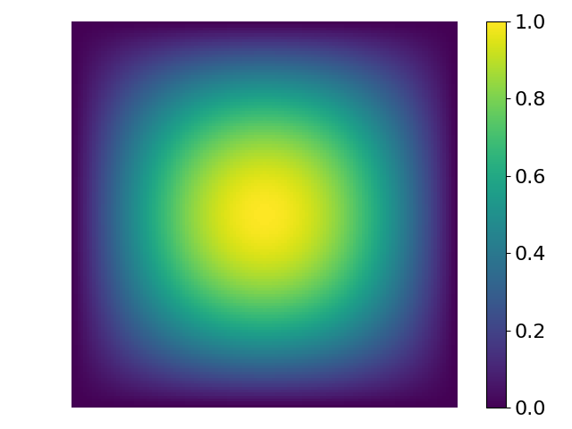
The data is similar in all numerical examples. In space, we consider a unit square domain, i.e., . The fine discretization is done with mesh size , while we vary the coarse mesh size for the convergence analysis. The temporal domain is discretized using a uniform time step and a final time . The diffusion coefficient is a piecewise constant function whose values vary on a scale of , such that clearly resolves the variations. We remark that the coefficient is generated once and remains the same through every realization of the equation. As initial data, we set , and the source function is constant . An illustration of the diffusion coefficient and the initial data can be seen in Figure 6.1.

For the implementation, it is necessary to construct a noise approximation of the -Wiener process . First of all, we define the trace class operator through the relation , where we set the eigenfunctions to , with corresponding eigenvalues . Here, the parameters and determine the amplitude and decay rate of the noise, respectively, and consequently affect the variance and smoothness of the corresponding solution. Moreover, recall the Karhunen–Loève expansion of in (2.3). For the numerical simulations, the common approach is to truncate such an expansion up to a truncation parameter . That is, the noise we consider for the examples is given by
| (6.3) |
where are mutually independent, real-valued Brownian motions. The truncation parameter is set to for all examples. This particular choice is common for the noise approximation in SPDE simulations and will not dominate the error if the eigenvalues of decay sufficiently fast (see, e.g., [8, 29]).
6.1. Strong convergence
In this part, we illustrate numerically the strong convergence derived in Theorem 4.4. For the noise, we have set the eigenvalues to as , and the truncation parameter to . For an illustration of one realization of the noise and the corresponding reference solution at final time , see Figure 6.2.
The LOD solution is computed for coarse spatial mesh sizes , , with localization parameter . We compare the error in -norm at final time against a reference solution computed with standard FEM on the fine grid. The norm is estimated by a Monte-Carlo estimator with 100 samples, i.e., . For comparison, the convergence rate when computing the coarse solution using standard FEM is also included, as well as an -reference line which indicates the sought convergence rate from Theorem 4.4. In the convergence plot in Figure 6.3, it is shown that the LOD solution achieves quadratic convergence, as predicted by Theorem 4.4, while the error for the FEM solution remains constant through all mesh sizes as it is unable to resolve the variations of .


6.2. Weak convergence
We study the convergence of the weak error between the expectation of the reference solution and its corresponding multiscale approximation. In order to compare the performance between the standard Monte-Carlo and the multilevel Monte-Carlo estimators, we fix for the standard Monte-Carlo estimation and denote by the LOD approximation on the coarse grid with mesh size . The term is estimated by applying a standard Monte-Carlo estimator and a multilevel Monte-Carlo estimator, respectively, in combination with the LOD method. To simplify the computations, we lower the variance from the previous example by choosing .
Remark 6.2.
The expectation of the solution to (6.1) does not in practice require an estimation via Monte-Carlo simulation. Due to the linearity, it holds that the expectation satisfies the deterministic equation
| (6.4) |
However, as shown in Section 5, the Monte-Carlo estimator can be used to approximate any Lipschitz continuous function of the solution to (6.1). In the example, we use the identity , since the reference solution can be computed using (6.4), which removes the issue of requiring a Monte-Carlo estimation for the reference solution.
In Section 5, it was shown how the Monte-Carlo error consists of the weak error and a statistical part, respectively. As an example, we compute for , , with samples on each mesh size, and show how the total error decays as a function of . This is illustrated in Figure 6.4, where we furthermore have included dashed horizontal lines that indicate the size of the deterministic error for each coarse mesh size. Note that after 10000 samples the statistical error has vanished for , while it is still present for . As pointed out in Section 5, the weak and statistical errors are balanced by choosing the samples of the Monte-Carlo estimator proportional to the mesh size as .
Next, we compute an estimation of using standard Monte-Carlo estimation and multilevel Monte-Carlo estimation, respectively, where the number of samples is chosen as a function of the coarse mesh size . In the following, we set as a scaling parameter for the number of samples. For the standard Monte-Carlo estimator we use number of samples. This is done for coarse mesh sizes , . For the multilevel Monte-Carlo estimator we set and let , for , with . This is done for mesh sizes , . The convergence of the weak error for both estimators is illustrated in Figure 6.6. For comparison, we have furthermore included the Monte-Carlo estimation of the finite element solution based on the coarse grid, i.e., with .
In the figure, we first of all note that both the Monte-Carlo and multilevel Monte-Carlo estimator of the LOD solution converge with quadratic rate, as predicted in Section 5. It is moreover shown that the finite element solution on the coarse grid is unable to reach the region of convergence as a consequence of not resolving the variations in the diffusion.
6.3. Computational complexity
We conclude with a note on the computational complexity of computing using the Monte-Carlo estimator and the multilevel estimator for the LOD method, and compare it with the standard Monte-Carlo estimation of the finite element method on the fine grid. As an example, we wish to compute the solution on an under-resolved grid with mesh size and let be sufficiently fine, i.e., it resolves the variations on the scale .
To simplify the presentation, we use the following notations. By and we denote the computational cost of solving a sparse matrix system defined by mesh sizes and , respectively. Furthermore, denotes the cost of computing a matrix system on the fine scale localized to the patch . Recall that the construction of the multiscale space consists of evaluating the basis correction for every node . In practice, this is done by solving number of fine (localized) system for each element . That is, the computational cost of evaluating the multiscale space based on the coarse mesh size is (see [19] for a more detailed discussion). However, we emphasize that this cost can be seen as an offline computation, and becomes of negligible size as the number of time steps and samples grow.
- FEM-MC:
For the Monte-Carlo estimation, we require number of samples of . For each sample, one must solve the system (2.31) number of times. In total, it is necessary to solve matrix systems defined on the fine grid with mesh size . The computational cost is thus .
- LOD-MC:
The Monte-Carlo estimator requires number of samples . To compute the samples, it is first necessary to construct the multiscale space . We emphasize that once this is done, the multiscale space can be re-used in each time step and for each sample. In total, we are required to solve for once, followed by solving matrix systems posed on defined by the coarse mesh size . The total cost is thus .
- LOD-MLMC:
For the multilevel estimator, we are first required to construct the multiscale spaces for the coarse mesh sizes , . Next, the estimator is computed, which requires samples of . At last, the estimators for are evaluated, which is done by computing samples of and , respectively. Recall that one sample of corresponds to sparse matrix systems defined by the grid size . In total, this adds to the computational cost
(6.5) where we have set .
Note that, although the FEM-MC and LOD-MC methods require the same number of samples , the LOD-MC computes the samples on the coarse scale while FEM-MC does so on the fine scale . We emphasize that the LOD-MLMC estimation is even more advantageous, since the number of samples computed on the scale is always , i.e., independent of the total number of samples. To illustrate the difference, the computational time for the simulations from the previous subsection were logged. This was done by taking the average computational time for one sample for each method, and multiplying it by the total number of samples. That is, for FEM-MC and LOD-MC, the number of samples are , and for the LOD-MLMC estimation we have and , with and . The computational times were computed for coarse mesh sizes and can be seen in Figure 6.6. Note that, for instance, the LOD-MC was never computed in the case in the previous subsection, due to computational limitations. However, since the computational time for one sample is known, it is possible to estimate the total time that is required for the entire estimation. In the figure, we note that the computational time for FEM-MC is magnitudes larger than each LOD-based method. The contrast between LOD-MC and LOD-MLMC is small for coarse mesh sizes, but as decreases the LOD-MLMC method shows significant advantage.
References
- [1] A. Abdulle, W. E, B. Engquist, and E. Vanden-Eijnden. The heterogeneous multiscale method. Acta Numer., 21:1–87, 2012.
- [2] R. Altmann, E. Chung, R. Maier, D. Peterseim, and S.-M. Pun. Computational multiscale methods for linear heterogeneous poroelasticity. J. Comput. Math., 38(1):41–57, 2020.
- [3] R. Altmann, P. Henning, and D. Peterseim. Numerical homogenization beyond scale separation. Acta Numer., 30:1–86, 2021.
- [4] A. Andersson, R. Kruse, and S. Larsson. Duality in refined Sobolev–Malliavin spaces and weak approximation of SPDE. Stoch. PDE: Anal. Comp., 4:113–149, 03 2016.
- [5] I. Babuška and R. Lipton. Optimal local approximation spaces for generalized finite element methods with application to multiscale problems. Multiscale Model. Simul., 9(1):373–406, 2011.
- [6] I. Babuška and J. E. Osborn. Generalized finite element methods: their performance and their relation to mixed methods. SIAM J. Numer. Anal., 20(3):510–536, 1983.
- [7] A. Barth and A. Lang. Multilevel Monte Carlo method with applications to stochastic partial differential equations. Int. J. Comput. Math, 89:2479 – 2498, 2012.
- [8] A. Barth and A. Lang. Simulation of stochastic partial differential equations using finite element methods. Stochastics, 84(2-3):217–231, 2012.
- [9] A. Barth, A. Lang, and C. Schwab. Multilevel Monte Carlo method for parabolic stochastic partial differential equations. BIT Numer. Math., 53(1):3–27, 2013.
- [10] D. Blömker, M. Hairer, and G. A. Pavliotis. Multiscale analysis for stochastic partial differential equations with quadratic nonlinearities. Nonlinearity, 20(7):1721–1744, 2007.
- [11] C.-E. Bréhier. Strong and weak orders in averaging for SPDEs. Stoch. Process. Their Appl., 122(7):2553–2593, 2012.
- [12] C.-E. Bréhier. Analysis of an HMM time-discretization scheme for a system of stochastic PDEs. SIAM J. Numer. Anal., 51(2):1185–1210, 2013.
- [13] C.-E. Bréhier. Orders of convergence in the averaging principle for SPDEs: The case of a stochastically forced slow component. Stoch. Process. Their Appl., 130(6):3325–3368, 2020.
- [14] S. C. Brenner. Two-level additive Schwarz preconditioners for nonconforming finite elements. Contemp. Math., 180:9–14, 1994.
- [15] G. Da Prato and J. Zabczyk. Stochastic Equations in Infinite Dimensions, volume 152 of Encyclopedia of Mathematics and its Applications. Cambridge University Press, Cambridge, second edition, 2014.
- [16] W. E and B. Engquist. The heterogeneous multiscale methods. Commun. Math. Sci., 1(1):87–132, 2003.
- [17] F. Edelvik, M. Görtz, F. Hellman, G. Kettil, and A. Mlqvist. Numerical homogenization of spatial network models. Preprint, arXiv:2209.05808, 2022.
- [18] Y. Efendiev, J. Galvis, and T. Y. Hou. Generalized multiscale finite element methods (GMsFEM). J. Comput. Phys., 251:116–135, 2013.
- [19] C. Engwer, P. Henning, A. Målqvist, and D. Peterseim. Efficient implementation of the localized orthogonal decomposition method. Comput. Methods Appl. Mech. Eng, 350:123–153, 06 2019.
- [20] A. Ern and J.-L. Guermond. Finite element quasi-interpolation and best approximation. ESAIM Math. Model. Numer. Anal., 51(4):1367–1385, 2017.
- [21] P. Freese, M. Hauck, and D. Peterseim. Super-localized orthogonal decomposition for high-frequency Helmholtz problems. Preprint, arXiv:2112.11368, 2021.
- [22] M. B. Giles. Multilevel Monte Carlo path simulation. Oper. Res., 56(3):607–617, 2008.
- [23] M. Hairer and D. Kelly. Stochastic PDEs with multiscale structure. Electron. J. Probab., 17:1–38, 2012.
- [24] M. Hauck and D. Peterseim. Super-localization of elliptic multiscale problems. Preprint, arXiv:2107.13211, 2021.
- [25] P. Henning and D. Peterseim. Oversampling for the multiscale finite element method. Multiscale Model. Simul., 11(4):1149–1175, 2013.
- [26] T. J. Hughes and J. R. Stewart. A space-time formulation for multiscale phenomena. J. Comput. Appl. Math., 74(1):217–229, 1996.
- [27] T. J. R. Hughes. Multiscale phenomena: Green’s functions, the Dirichlet-to-Neumann formulation, subgrid scale models, bubbles and the origins of stabilized methods. Comput. Methods Appl. Mech. Engrg., 127(1-4):387–401, 1995.
- [28] T. J. R. Hughes, G. R. Feijóo, L. Mazzei, and J.-B. Quincy. The variational multiscale method – a paradigm for computational mechanics. Comput. Methods Appl. Mech. Engrg., 166(1-2):3–24, 1998.
- [29] M. Kovács, S. Larsson, and F. Lindgren. Strong convergence of the finite element method with truncated noise for semilinear parabolic stochastic equations with additive noise. Numer. Algorithms, 53(2-3):309–320, 2010.
- [30] M. Kovács, S. Larsson, and F. Lindgren. Weak convergence of finite element approximations of linear stochastic evolution equations with additive noise. BIT Numer. Math., 52:85–108, 2012.
- [31] R. Kruse. Strong and Weak Approximation of Semilinear Stochastic Evolution Equations, volume 2093 of Lecture Notes in Mathematics. Springer Cham, 2014.
- [32] R. Kruse and S. Larsson. Optimal regularity for semilinear stochastic partial differential equations with multiplicative noise. Electron. J. Probab., 17(65):1–19, 2012.
- [33] A. Lang and A. Petersson. Monte Carlo versus multilevel Monte Carlo in weak error simulations of SPDE approximations. Math. Comput. Simul., 143:99–113, 2018.
- [34] S. Larsson and V. Thomée. Partial Differential Equations with Numerical Methods. Texts in Applied Mathematics. Springer, 2003.
- [35] W. Liu and M. Röckner. Stochastic Partial Differential Equations: An Introduction. Universitext. Springer International Publishing, 2015.
- [36] P. Ljung, R. Maier, and A. Mlqvist. A space-time multiscale method for parabolic problems. SIAM Multiscale Model. Simul., 20(2):714–740, 2022.
- [37] G. J. Lord, C. E. Powell, and T. Shardlow. An Introduction to Computational Stochastic PDEs. Cambridge Texts in Applied Mathematics. Cambridge University Press, 2014.
- [38] S. Lototsky and B. Rozovsky. Stochastic Partial Differential Equations. Springer, 2017.
- [39] A. Mlqvist and A. Persson. A generalized finite element method for linear thermoelasticity. ESAIM Math. Model. Numer. Anal., 51(4):1145–1171, 2017.
- [40] A. Mlqvist and A. Persson. Multiscale techniques for parabolic equations. Numer. Math., 138(1):191–217, 2018.
- [41] A. Mlqvist and D. Peterseim. Localization of elliptic multiscale problems. Math. Comp., 83(290):2583–2603, 2014.
- [42] A. Mlqvist and D. Peterseim. Numerical homogenization by localized orthogonal decomposition, volume 5 of SIAM Spotlights. Society for Industrial and Applied Mathematics (SIAM), Philadelphia, PA, 2020.
- [43] A. Målqvist and D. Peterseim. Computation of eigenvalues by numerical upscaling. Numer. Math., 130:337–361, 2015.
- [44] P. Oswald. On a BPX-preconditioner for P1 elements. Computing, 51(2):125–133, 1993.
- [45] H. Owhadi. Multigrid with rough coefficients and multiresolution operator decomposition from hierarchical information games. SIAM Rev., 59(1):99–149, 2017.
- [46] H. Owhadi and C. Scovel. Operator-Adapted Wavelets, Fast Solvers, and Numerical Homogenization, volume 35 of Cambridge Monographs on Applied and Computational Mathematics. Cambridge University Press, Cambridge, 2019.
- [47] A. Pazy. Semigroups of Linear Operators and Applications to Partial Differential Equations. Applied mathematical sciences. Springer, 1983.
- [48] V. Thomée. Galerkin Finite Element Methods for Parabolic Problems, volume 25 of Springer Series in Computational Mathematics. Springer, 1997.
- [49] Y. Yan. Semidiscrete galerkin approximation for a linear stochastic parabolic partial differential equation driven by an additive noise. BIT Numer. Math., 44(4):829–847, 2004.
- [50] Y. Yan. Galerkin finite element methods for stochastic parabolic partial differential equations. SIAM J. Numer. Anal., 43(4):1363–1384, 2005.