Quantum Measurement Spintronic Engine powered by Quantum Fluctuations

In the emerging field of quantum thermodynamics Vinjanampathy and Anders 2016 and specifically of quantum energetics Rogers and Jordan 2022, much effort has been dedicated to the study of quantum thermal machines and quantum batteries Bhattacharjee and Dutta 2021, in the hope of finding new ways of producing energy at the nanoscale. A first approach describes quantum analogues to a classical engines that rely either on a Maxwell demon Ptaszyński 2018; Seah et al. 2020, a cycle between different baths Piccitto et al. 2022; Manzano et al. 2016; Molitor and Landi 2020 or an external drive Donvil 2018; Zhao et al. 2021; Santos and Santos 2022. A second approach focuses on systems that specifically rely on quantum features such as coherence Francica et al. 2020; Shi et al. 2020; Aimet and Kwon 2023; Monsel et al. 2020 and entanglement Buffoni et al. 2019; Bresque et al. 2021; Jussiau et al. in order to extract energy from the environment using the singular properties of quantum superposition and quantum measurements. These new kinds of quantum engines which have been demonstrated experimentally Katcko et al. 2019; Chowrira et al. 2022; Klatzow et al. 2019; Ji et al. 2022; Micadei et al. 2019 redefine the notion of temperature when examining engine efficiencies against the Carnot limit Niedenzu et al. 2018; Roßnagel et al. 2014; Manzano et al. 2016; Klaers et al. 2017, notably when harvesting energy from single heat baths Scully 2003; Yi et al. 2017.

Quantum measurements constitute a critical process that could lead to active devices that use entanglement as a fuel Elouard and Jordan 2018; Francica et al. 2017. Indeed, the resulting projection that such a measurement performs on a quantum state involves an irreversible energy exchange between that state and the environment Rogers and Jordan 2022 that can be viewed as a form of quantum heat Elouard et al. 2017. The information obtained from the measurement can either be used by a Maxwell demon Elouard et al. 2017; Bresque et al. 2021 that can extract energy by applying some unitary transformation to the working substance (WS), or the measurement back-action in itself can result in an energy increase that can be harvested into usable work Yi et al. 2017.

In these engine models Piccitto et al. 2022; Jussiau et al.; Klaers et al. 2017; Molitor and Landi 2020; Ptaszyński 2018; Seah et al. 2020; Francica et al. 2020; Shi et al. 2020; Aimet and Kwon 2023; Niedenzu et al. 2018; Roßnagel et al. 2014; Manzano et al. 2016; Klaers et al. 2017; Henriet et al. 2015, the proposed cycle can be difficult to implement experimentally, while the cost of turning on/off interactions between the WS and the baths is ignored. In this Letter, we model a quantum electronic engine that mostly lifts these limitations, that is explicitly powered by quantum fluctuations in contrast to recent proposals Jussiau et al.; Xiao et al., and that advantageously mimics a recent experimental implementation Katcko et al. 2019; Chowrira et al. 2022.

This quantum spintronic engine’s WS is composed of two spin-split quantum dots (QDs) that exhibit a tunnel coupling $\gamma$, a magnetic exchange interaction $J$, and coulombic repulsion $U$ to prevent excessive charging. This open system is connected in series with two ferromagnetic, fully spin-polarized leads. Since the engine is a solid-state device, electronic interactions are inherently always on and time-independent, such that the engine cycle is only driven by periodic quantum measurements through two strokes : an instantaneous measurement stroke that partially projects the QD system (i.e. WS), followed by a thermalizing stroke of duration $\tau$ during which the WS relaxes towards the steady-state.

Our initial formalism follows prior literature Fransson and Råsander 2006; Weymann and Barnaś 2007; Fransson et al. 2014, and was used to successfully model magnetotransport across a quantum spintronic engine under the assumption of effective work Katcko et al. 2019.

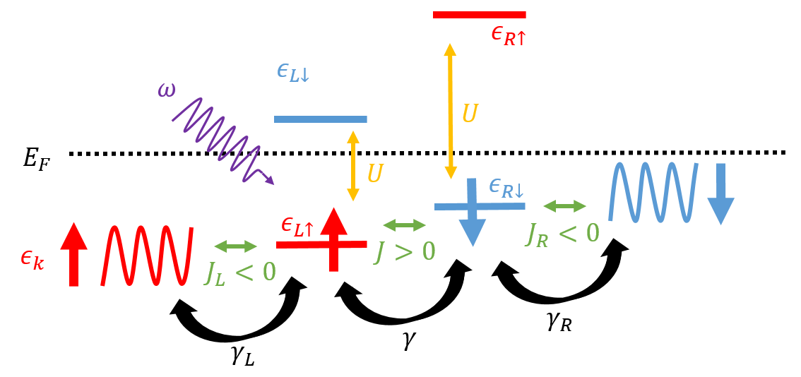
Model.—In line with experimental input Katcko et al. 2019; Chowrira et al. 2022, we make the following assumptions: $J<0$, $\gamma$ is spin-independent, only one electronic band is involved, the spintronic anisotropy remains constant (no external bias voltage), the $\uparrow$ spin energy level on the right side is inaccessible, and the tunnelling coefficients $\gamma_{L}$ and $\gamma_{R}$ are asymmetric. We can thus simplify the system (see schematic in Fig. 1 and SI note 1), so that the system Hamiltonian reads:

where $c_{\downarrow}$, $c_{\uparrow}$ and $c_{R}$ are the annihilation operators of the left $\downarrow$ spin, the left $\uparrow$ spin and the right $\downarrow$ spin respectively ; $n=c^{\dagger}c$ are the number operators and $\epsilon$ are the effective bare energy of each electronic level. Note the absence of an explicit spin channel between the electrodes, and of a spin-flip mechanism ; hence our model can lead to electron transport through engine operation that can only arise from so-called quantum fluctuations via two-electron processes.

In SI Note. 1, we establish the master equation describing the evolution of this open quantum system:

where $\rho_{S}=\mathrm{Tr}_{E}\,\rho$ is the QD system’s reduced density matrix w.r.t the environment degrees of freedom, $\mathcal{T}^{-}_{L}$ and $\mathcal{T}^{-}_{R}$ represent the electron hopping intensity beteen the QD and the left/right lead respectively, while $\mathcal{T}^{+}_{L}$ and $\mathcal{T}^{+}_{R}$ are the hole counterparts; and with the superoperator $\mathcal{D}[c](\rho)\equiv c\rho c^{\dagger}-\frac{1}{2}\{c^{\dagger}c,\rho\}$.

A key element of our quantum spintronic engine is the ferromagnetic metal/molecule interface. This so-called spinterface exhibits a low density of spatiospectrally confined states with high spin polarization (89% Chowrira et al. 2022) at the Fermi level Djeghloul et al. 2016; Delprat et al. 2018; Katcko et al. 2019; Chowrira et al. 2022. The proposal that a Maxwell demon can operate electronically at the molecular level Bergfield et al. 2013, along with recent thermodynamical theory on quantum measurements Manzano et al. 2018; Erez et al. 2008; Erez 2012, indicate that the spinterface could Chowrira et al. 2022 act as an autonomous quantum measurement apparatus by performing frequent projective measurements on the nearby QD, thereby collapsing the WS’s quantum state Lindblad 1973; Jacobs 2012; Ban 1999. Following related studies that all postulate an external non-thermal input quantum resource Scully 2003; Bresque et al. 2021; Jussiau et al.; Elouard et al. 2017; Yi et al. 2017, we assume that the spinterface can perform these quantum measurements without an energy cost. Here, however, this assumption is backed by the ability of the ferromagnetic electrode to maintain a constant spin polarization, thus allowing it to behave as an entropy sink. Indeed, information erasure would require a much lower entropy cost than the Landauer bound by involving the transfer of spin angular momentum into a large spin reservoir, rather than energy Wright et al. 2018; Bormashenko 2020; Vaccaro and Barnett 2011.

Engine.—Using our Hamiltonian, we consider a two-phased engine cycle (see Fig. 2). A first ’thermalizing’ stroke places the QDs into equilibrium with the electrode baths. The relaxation of the QD sytems during this time-dependent evolution transfers energy from the system to the baths, some of which is harvested to produce useful electrical work. Then, once the system reaches its entangled steady-state, a ’measurement’ stroke on a single QD splits the WS into two separated subsystems, thereby killing the entanglement. As we will show, this projective partial unselective measurement acting on a superposed mixed stated with indefinite energy is mathematically described by a quantum channel that leads to a projected system with a higher mean energy than the previous steady-state. The excess energy that results from this back-action Bresque et al. 2021; Seah et al. 2020; Yi et al. 2017 of the measurement is then dissipated into the baths during the next ’thermalizing’ stroke. We will show that it can be used to produce electrical work.

To find the equilibrium state, we first derive the density matrix $\rho\equiv\rho_{ss}$ such as $\frac{\mathrm{d}\rho}{\mathrm{d}t}=0$ so that $\rho$ nullify the right hand side of Eq.2. To obtain an approximate analytical solution, we use a perturbation approach on $\gamma$ (see SI Note 2), i.e. assume that other interaction energies dominate Chowrira et al. 2022 the hybridization between the QDs. The solution is given by an affine space, parameterized by the initial population $\mu=\langle n_{\downarrow}(0)\rangle$ of the spin $\downarrow$ energy level on the left QD. Upon choosing the basis:

we obtain the full density matrix $\rho^{\mu}$ after thermalization:

where $\beta^{\mu}\equiv\mu\mathcal{T}_{R}^{+}-(1-\mu)\mathcal{T}_{R}^{-}$, $1/\alpha\equiv(\mathcal{T}_{L}^{+}+\mathcal{T}_{L}^{-})(\mathcal{T}_{R}^{+}+\mathcal{T}_{R}^{-})$, $\Delta\equiv\epsilon_{\downarrow}-\epsilon_{R}$, $B$ is referenced in SI Note. 2 and the other terms are null.

Let us initialize our engine at $t_{0}=0$ in some state $\rho(0)$ such that $\mu=\langle n_{\downarrow}(0)\rangle$. After completing a first thermalization process, the electrode performs a partial projective measurement of the entangled QDs at time $t_{1}=\tau_{m}\equiv\tau$, which represents the duration of one cycle. This measurement projects the system from the steady state $\rho(\tau^{-})=\rho^{\mu}\equiv\rho$ to a projected state $\rho(\tau^{+})$ that depends on the measurement outcome. Supposing that the right electrode operates frequent unselective measurements of the occupation of the right QD at times $t=t_{n}\equiv n\tau$, the associated observable is simply $n_{R}$. The measurement yields either the presence ($n_{R}$ = 1) or the absence ($n_{R}$ = 0) of one electron on the right-hand QD. The two possible projectors on the respective eigenspaces are $\Pi_{0}=1-n_{R}$ and $\Pi_{1}=n_{R}$, leading to the projected state:

Using the following expression for the density matrix,

we immediately witness that the off-diagonal terms do not contribute in the projected state because they encode the tunnelling of one electron from one site to the next, leaving either the initial state or the final state with no electron on the right side. Hence we calculate $\rho(\tau^{+})=\sum_{i=0}^{7}\rho_{ii}|i\rangle\langle i|$ so that $\rho(\tau^{+})$ is the diagonal part of $\rho$, while $-2\mathcal{D}[n_{R}](\rho)$ is the off-diagonal part.

We can now calculate the energy and entropy impact of the measurement. The average energy of the system changes by an amount $\Delta E$:

which thus represents the energy of the off-diagonal part:

where $T\equiv\gamma c_{\downarrow}^{\dagger}c_{R}+\gamma^{*}c_{R}^{\dagger}c_{\downarrow}$ is the inter-dot tunnel operator. Thus, the measurement induces a back-action on the system by disentangling it, leading to an energy change $\Delta E$ compared to the thermalized state.

To study the thermalized state of the next cycle, we consider the particle number with spin $\downarrow$ in the left QD. Since the projected state is diagonal, we directly obtain:

So, for both measurement outcomes, the spin $\downarrow$ occupation number remains unchanged after both the thermalizing and measurement strokes. Therefore, the second cycle starts again with $\langle n_{\downarrow}(\tau^{+})\rangle=\mu$, and so yields the same thermalized state just before the second measurement , such that $\rho(2\tau^{-})=\rho(\tau^{-})=\rho$ and thus an instant recursion yields the system state after each cycle $n$:

This shows that at time $t=n\tau^{+}$, the system has received a total average energy $n\Delta E$ from quantum measurements. Therefore, if $\Delta E>0$, then the measurement on average energizes the system, and a fraction of that energy upon deexciting to the thermalized state can be harvested in the form of electron transport.

In SI Note. 3, we show that the engine operation/output is unchanged when measuring an observable that acts on only one QD (e.g. when the occupation of the left QD, or the charge (or spin) of the right QD, is measured). Measuring an observable that operates on both QDs, such as the total charge, does not yield this energy increment: the thermalized and measured states both present the same average energy. Work extraction from these cycles is possible only when the measurement separates the two QDs. Then, in SI Note. 4, we study the case of selective quantum measurements and show that the energy increment relation holds by linearity while entropic considerations differ.

We can express the energy $\Delta E=-2\Re[\gamma(\rho_{14}+\rho_{36})]$ associated with the measurement back-action as:

with $s\equiv\mathcal{T}_{L}^{+}+\mathcal{T}_{L}^{-}$, $m\equiv\mathcal{T}_{L}^{-}$, $r\equiv\frac{\mathcal{T}_{R}^{+}+\mathcal{T}_{R}^{-}}{2}$. To study $\Delta E$, we first assume (see SI. Note 1) that all the energies involved in the system $\mathcal{T}_{L}^{+}$, $\mathcal{T}_{L}^{-}$, $\mathcal{T}_{R}^{+}$, $\mathcal{T}_{R}^{-}$, $\Delta$ and $U$ are strictly positive. This immediately leads to $s,m,r>0$ and then to $\Delta E$ having the same sign as $\beta^{\mu}$. Therefore, the measurement energizes the two QDs whenever $\mu<\frac{\mathcal{T}_{R}^{-}}{\mathcal{T}_{R}^{+}+\mathcal{T}_{R}^{-}}\equiv\mu^{c}$.

We emphasize that the engine is still bounded by a Carnot limit. Indeed, in SI Note. 5, we define the engine efficiency $\eta\equiv\frac{W_{el}}{\Delta E}$, where $W_{el}$ is the electronic work obtained during the thermalization process, and we show that $\eta\leqslant 1-\frac{T}{T_{c}}$. Here, the critical temperature $T_{c}\equiv\frac{\Delta E}{\Delta S}$ defines a threshold above which this engine cannot operate, and $\Delta S>0$ is the difference of Von-Neumann entropy between the measured state and the steady-state.

Simulations.—To evaluate these analytical results, we simulated the engine operation in order to witness the drift from the perturbative solution, and to show that the measurement reliably provides energy over many cycles. We present in Fig. 3 the results of measuring $n_{R}$ across $10^{6}$ cycles (see also SI Note. 6). Starting from the pure state $\rho_{0}=|\uparrow\downarrow\rangle\langle\uparrow\downarrow|$, we first see that the identity $\Delta E=-\langle T\rangle$ is well respected (see Fig.SI.1), and that $\Delta E$ decreases after each cycle (see Fig. 3(a)). This is because the population of the down spin $\mu=\langle n_{\downarrow}\rangle$ gradually increases up to $\mu^{c}=1/2$ in this case, drifting away from the approximate solution that considers it constant to first order in $\gamma$. This equilibration therefore reduces the magnitude of the off-diagonal terms that code for the energizing process, as they are proportional to $\beta^{\mu}$ (see SI Note. 2). Choosing different values for $\mathcal{T}_{R}^{+}$ and $\mathcal{T}_{R}^{-}$ should therefore favor a higher energizing capability. The perturbative solution we derived to approximate the state after each thermalizing stroke deviates from the numerical solution but it correctly mimicks how observables evolve, even after many cycles. Note that the solution should be used each time with a different parameter $\mu$ obtained from the numerically measured state (see Fig. 3(c)).

The simulation strongly depends on the the initial state $\rho_{0}$. In Fig. 3(c) and (d), we show that, starting from a mixed state $\rho_{0}=\frac{1}{2}|\uparrow\downarrow\rangle\langle\uparrow\downarrow|+\frac{1}{2}|\downarrow\downarrow\rangle\langle\downarrow\downarrow|$, we instead find that $\Delta E$ oscillates randomly between two values. We conjecture that, after a long time, the engine initialized with $\rho_{0}=|\uparrow\downarrow\rangle\langle\uparrow\downarrow|$ will approach this fluctuating behavior around 0, as the information on the initial condition is progressively lost through the non-unitary system evolution during thermalization. This eventually leads to nearly vanishing power output due to excessive entropy: the temporal average energy increment falls from $\mathbb{E}[\Delta E]=10^{-6}$ meV to $\mathbb{E}[\Delta E]=10^{-9}$ meV. See SI Note 5 for additional data exploring different parameters, measurement protocols, as well as the case of selective measurements. These results show similar behaviors, i.e. all exhibit the ability to extract energy.

We now consider cases outside the perturbative regime detailed above. First, in SI Note. 7, we showed that for a wide range of parameters, it is unreasonable to approximate the state at the end of the thermalizing stroke as the steady-state solution.Thus, in this general case, we can only hope to reach a partial thermalization, though it may be beneficial to the power output of the device. Indeed, statistics (not shown) on the steady-state entanglement energy reveal that, at infinite time $|\langle T\rangle|\approx 10^{-9}-10^{-16}$ meV for standard parameter ranges, while after $t=1$ meV${}^{-1}\approx 4$ ps, we can reach up to $|\langle T\rangle|\approx 10^{3}$ meV for the same parameter ranges and for specific initial conditions. This suggests a higher energy increment. Indeed, the average energy increment per cycle is still given by $\Delta E=-\langle T\rangle$ in this general case, so that the previous energetic description of the cycle remain valid here. A proof of this assertion is given in SI Note. 8 along with a numerical justification based on measurement statistics.

To study how the parameters that impact the steady-state $\rho$ affect the entanglement energy $-\langle T\rangle$, we present In Fig. 4 several color plots of $-\langle T\rangle$ calculated after partial thermalization starting from the pure state $\rho_{0}=|\uparrow\downarrow\rangle\langle\uparrow\downarrow|$ as a function of the most relevant different pairs of parameters (see SI Note. 9 for other plots), while keeping other parameters fixed, and with $\gamma\gg U\sim\epsilon\sim\mathcal{T}$. In Fig 4(a), we notice that $-\langle T\rangle$ is maximized when $U\approx 10^{4}$ and $\mathcal{T}_{L}^{+}=\mathcal{T}_{L}^{-}<1$. Indeed, a higher $U$ could lead to a bigger entanglement energy that is related to the charging energy of a QD, while a lower $\mathcal{T}_{L}$ favors the tunneling between the QDs over the tunneling from/to the electrodes. In Fig 4(b), we observe that the asymmetry between $\mathcal{T}_{L}$ and $\mathcal{T}_{R}$ is completely irrelevant for this set of parameters for low $\mathcal{T}_{R}$: the engine generates power and energy harvesting may be possible. Above a phase transition around $\mathcal{T}_{R}\approx 10$ (see also Fig 4(d)), a chaotic phase ensues, the value of $\langle T\rangle$ almost vanishes and its sign strongly depends on small fluctuations of the parameters: we cannot hope to extract energy in this configuration. In Fig 4(c), we examine the electron/hole asymmetry on the right electrode. The data reveals a third phase in white in which $-\langle T\rangle<0$: a dissipative phase with no energy extraction. Finally, in Fig 4(d), the $U$ / $\gamma$ dependence reveals two branches that maximize $-\langle T\rangle$: one for $\gamma\approx 1$ that weakly depends on $U$, and a second for $\gamma\approx U$. This may help tune experimental device parameters to maximize energy harvesting.

Using the data of SI Note. 9, we infer a regime wherein the entanglement energy is highest when $\mathcal{T}\ll\epsilon\ll\gamma\approx U\approx 1000\epsilon$. To confirm the high power output $P=\frac{\mathbb{E}[\Delta E]}{\tau}$ within this parameter space, we simulated $10^{6}$ engine cycles (see plots in Fig 5). Strikingly, we observe strong fluctuations of $\Delta E$ that ultimately kill the temporal average of the energy increment. This shows that maximizing $-\langle T\rangle$ also yields a strong dependence of the tunneling energy after partial thermalization on the initial conditions. This increases the fluctuations and negatively impacts $P$: maximizing $P$ requires balancing energy and fluctuations. Indeed, from the Heisenberg uncertainty relations, when selectively measuring $n_{R}$, we may write:

Here, at the end of each cycle, $\Delta n_{R}\lesssim 1$ is known and fixed by the statistical outcomes of the measurements and should be of order unity since the measurement alternatively projects the system into a $n_{R}=$ 0 or 1 state. Moreover, the right-hand side describes the $n_{R}$ oscillation rate, which is strongly driven by the $|\langle T\rangle|$ energy scale. Thus, Eq. 12 indeed justifies that $\Delta T\gtrsim|\langle T\rangle|$.

Conclusions.—We studied a quantum information engine built around autonomous solid-state spintronic interactions that can promote the energy harvesting of quantum fluctuations. Our model considered a pair of entangled spin quantum dots that electronically interact with spin-selecting electrodes. By using physical assumptions from prior experimentsKatcko et al. 2019; Chowrira et al. 2022 to reduce parameter space, we derived a master equation that describes a two-cycle engine featuring: a thermalizing stroke that entangles the two quantum dots and generates electron transport, then a quantum measurement stroke that extracts energy from their mutual information, i.e. through quantum separation. This changes their entropy by separating and projecting the system in a higher energy state on average. In the limiting case that quantum fluctuationsconstitute the only energy source, numerical simulations predicted a finite appreciable power output in some cases. The far lower magnitude compared with experiments Chowrira et al. 2022 is either due to a faster thermalization, or to another energy source such as phonons. Our work opens fruitful research into spintronic interaction dynamics between ferromagnets and paramagnetic centers Bowen 2023, e.g. using scanning tunnelling and ferromagnetic resonance techniques Harder et al. 2016, to elucidate the thermodynamic role Vaccaro and Barnett 2011; Wright et al. 2018 of the ferromagnetic metal / molecule quantum measurement apparatusKatcko et al. 2019; Chowrira et al. 2022. Our model’s autonomous interlocking electronic strokes to generate feedback on quantum entanglement should inspire the fields of quantum chemistryLi and Kais 2019, biology Kim et al. 2021 and cognition Adams and Petruccione 2020.

We thank C. Elouard, J. Monsel, K. Singer, and R. Whitney for stimulating discussions. We gratefully acnkowledge PhD funding for M.L. from Ecole Polytechnique. We acknowledge financial support from the ANR (ANR-21-CE50-0039), the Contrat de Plan Etat-Region grants in 2006 and 2008, by “NanoTérahertz”, a project co-funded by the ERDF 2014–2020 in Alsace (European Union fund) and by the Region Grand Est through its FRCR call, by the impact project LUE-N4S part of the French PIA project “Lorraine Université d’Excellence”, reference ANR-15IDEX-04-LUE and by the FEDER-FSE “Lorraine et Massif Vosges 2014–2020”, a European Union Program. This ‘SpinDrive’ work of the Interdisciplinary Thematic Institute QMat, as part of the ITI 2021-2028 program of the University of Strasbourg, CNRS and Inserm, was supported by IdEx Unistra (ANR 10 IDEX 0002), and by SFRI STRAT’US project (ANR 20 SFRI 0012) and EUR QMAT ANR-17-EURE-0024 under the framework of the French Investments for the Future Program.

SUPPLEMENTARY INFORMATION
Quantum Measurement Spintronic Engine powered by Quantum Fluctuations

Mathieu Lamblin and Martin Bowen

SUPPLEMENTARY INFORMATION
Quantum Measurement Spintronic Engine powered by Quantum Fluctuations

Mathieu Lamblin Martin Bowen

August 11, 2026

References

- Klatzow et al. (2019) J. Klatzow, J. N. Becker, P. M. Ledingham, C. Weinzetl, K. T. Kaczmarek, D. J. Saunders, J. Nunn, I. A. Walmsley, R. Uzdin, and E. Poem, Experimental Demonstration of Quantum Effects in the Operation of Microscopic Heat Engines, Physical Review Letters 122, 10.1103/PhysRevLett.122.110601 (2019).
- Bresque et al. (2021) L. Bresque, P. A. Camati, S. Rogers, K. Murch, A. N. Jordan, and A. Auffèves, Two-Qubit Engine Fueled by Entanglement and Local Measurements, Physical Review Letters 126, 10.1103/PhysRevLett.126.120605 (2021).
- (3) E. Jussiau, L. Bresque, A. Auffeves, K. W. Murch, and A. N. Jordan, Many-body quantum vacuum fluctuation engines, , 19.
- Katcko et al. (2019) K. Katcko, E. Urbain, B. Taudul, F. Schleicher, J. Arabski, E. Beaurepaire, B. Vileno, D. Spor, W. Weber, D. Lacour, S. Boukari, M. Hehn, M. Alouani, J. Fransson, and M. Bowen, Spin-driven electrical power generation at room temperature, Communications Physics 2, 10.1038/s42005-019-0207-8 (2019).
- Chowrira et al. (2022) B. Chowrira, L. Kandpal, M. Lamblin, F. Ngassam, C. Kouakou, T. Zafar, D. Mertz, B. Vileno, C. Kieber, G. Versini, B. Gobaut, L. Joly, T. Ferté, E. Monteblanco, A. Bahouka, R. Bernard, S. Mohapatra, H. Prima Garcia, S. Elidrissi, M. Gavara, E. Sternitzky, V. Da Costa, M. Hehn, F. Montaigne, F. Choueikani, P. Ohresser, D. Lacour, W. Weber, S. Boukari, M. Alouani, and M. Bowen, Quantum Advantage in a Molecular Spintronic Engine that Harvests Thermal Fluctuation Energy, Advanced Materials 34, 2206688 (2022).
- Wright et al. (2018) J. S. S. T. Wright, T. Gould, A. R. R. Carvalho, S. Bedkihal, and J. A. Vaccaro, Quantum heat engine operating between thermal and spin reservoirs, Physical Review A 97, 10.1103/PhysRevA.97.052104 (2018).
- Li and Kais (2019) J. Li and S. Kais, Entanglement classifier in chemical reactions, Science Advances 5, 10.1126/sciadv.aax5283 (2019).
- Kim et al. (2021) Y. Kim, F. Bertagna, E. M. D’Souza, D. J. Heyes, L. O. Johannissen, E. T. Nery, A. Pantelias, A. S.-P. Jimenez, L. Slocombe, M. G. Spencer, J. Al-Khalili, G. S. Engel, S. Hay, S. M. Hingley-Wilson, K. Jeevaratnam, A. R. Jones, D. R. Kattnig, R. Lewis, M. Sacchi, N. S. Scrutton, S. R. P. Silva, and J. McFadden, Quantum biology: An update and perspective, Quantum Reports 3, 80 (2021).
- Adams and Petruccione (2020) B. Adams and F. Petruccione, Quantum effects in the brain: A review, AVS Quantum Science 2, 022901 (2020).
- Vinjanampathy and Anders (2016) S. Vinjanampathy and J. Anders, Quantum thermodynamics, CONTEMPORARY PHYSICS 57, 545 (2016).
- Rogers and Jordan (2022) S. Rogers and A. N. Jordan, Postselection and quantum energetics, Physical Review A 106, 10.1103/PhysRevA.106.052214 (2022).
- Bhattacharjee and Dutta (2021) S. Bhattacharjee and A. Dutta, Quantum thermal machines and batteries, The European Physical Journal B 94, 10.1140/epjb/s10051-021-00235-3 (2021).
- Ptaszyński (2018) K. Ptaszyński, Autonomous quantum Maxwell’s demon based on two exchange-coupled quantum dots, Physical Review E 97, 10.1103/PhysRevE.97.012116 (2018).
- Seah et al. (2020) S. Seah, S. Nimmrichter, and V. Scarani, Maxwell’s Lesser Demon: A Quantum Engine Driven by Pointer Measurements, Physical Review Letters 124, 10.1103/PhysRevLett.124.100603 (2020).
- Piccitto et al. (2022) G. Piccitto, M. Campisi, and D. Rossini, The ising critical quantum otto engine, New Journal of Physics 24, 10.1088/1367-2630/ac963b (2022).
- Manzano et al. (2016) G. Manzano, F. Galve, R. Zambrini, and J. M. R. Parrondo, Entropy production and thermodynamic power of the squeezed thermal reservoir, Physical Review E 93, 10.1103/PhysRevE.93.052120 (2016).
- Molitor and Landi (2020) O. A. D. Molitor and G. T. Landi, Stroboscopic two-stroke quantum heat engines, Physical Review A 102, 10.1103/PhysRevA.102.042217 (2020).
- Donvil (2018) B. Donvil, Thermodynamics of a periodically driven qubit, Journal of Statistical Mechanics: Theory and Experiment 2018, 043104 (2018).
- Zhao et al. (2021) F. Zhao, F.-Q. Dou, and Q. Zhao, Quantum battery of interacting spins with environmental noise, Physical Review A 103, 10.1103/PhysRevA.103.033715 (2021).
- Santos and Santos (2022) T. F. F. Santos and M. F. Santos, Efficiency of optically pumping a quantum battery and a two-stroke heat engine, Phys. Rev. A 106, 052203 (2022).
- Francica et al. (2020) G. Francica, F. Binder, G. Guarnieri, M. Mitchison, J. Goold, and F. Plastina, Quantum Coherence and Ergotropy, Physical Review Letters 125, 10.1103/PhysRevLett.125.180603 (2020).
- Shi et al. (2020) Y.-H. Shi, H.-L. Shi, X.-H. Wang, M.-L. Hu, S.-Y. Liu, W.-L. Yang, and H. Fan, Quantum coherence in a quantum heat engine, Journal of Physics A-Mathematical and Theoretical 53, 10.1088/1751-8121/ab6a6b (2020).
- Aimet and Kwon (2023) S. Aimet and H. Kwon, Engineering a heat engine purely driven by quantum coherence, Phys. Rev. A 107, 012221 (2023).
- Monsel et al. (2020) J. Monsel, M. Fellous-Asiani, B. Huard, and A. Auffèves, The Energetic Cost of Work Extraction, Physical Review Letters 124, 10.1103/PhysRevLett.124.130601 (2020).
- Buffoni et al. (2019) L. Buffoni, A. Solfanelli, P. Verrucchi, A. Cuccoli, and M. Campisi, Quantum Measurement Cooling, Physical Review Letters 122, 10.1103/PhysRevLett.122.070603 (2019).
- Ji et al. (2022) W. Ji, Z. Chai, M. Wang, Y. Guo, X. Rong, F. Shi, C. Ren, Y. Wang, and J. Du, Spin Quantum Heat Engine Quantified by Quantum Steering, Physical Review Letters 128, 10.1103/PhysRevLett.128.090602 (2022).
- Micadei et al. (2019) K. Micadei, J. P. S. Peterson, A. M. Souza, R. S. Sarthour, I. S. Oliveira, G. T. Landi, T. B. Batalhão, R. M. Serra, and E. Lutz, Reversing the direction of heat flow using quantum correlations, Nature Communications 10, 10.1038/s41467-019-10333-7 (2019).
- Niedenzu et al. (2018) W. Niedenzu, V. Mukherjee, A. Ghosh, A. G. Kofman, and G. Kurizki, Quantum engine efficiency bound beyond the second law of thermodynamics, Nature Communications 9, 10.1038/s41467-017-01991-6 (2018).
- Roßnagel et al. (2014) J. Roßnagel, O. Abah, F. Schmidt-Kaler, K. Singer, and E. Lutz, Nanoscale heat engine beyond the carnot limit, Physical review letters 112, 030602 (2014).
- Klaers et al. (2017) J. Klaers, S. Faelt, A. Imamoglu, and E. Togan, Squeezed Thermal Reservoirs as a Resource for a Nanomechanical Engine beyond the Carnot Limit, Physical Review X 7, 10.1103/PhysRevX.7.031044 (2017).
- Scully (2003) M. O. Scully, Extracting Work from a Single Heat Bath via Vanishing Quantum Coherence, Science 299, 862 (2003).
- Yi et al. (2017) J. Yi, P. Talkner, and Y. W. Kim, Single-temperature quantum engine without feedback control, Physical Review E 96, 10.1103/PhysRevE.96.022108 (2017).
- Elouard and Jordan (2018) C. Elouard and A. N. Jordan, Efficient Quantum Measurement Engines, Physical Review Letters 120, 10.1103/PhysRevLett.120.260601 (2018).
- Francica et al. (2017) G. Francica, J. Goold, F. Plastina, and M. Paternostro, Daemonic ergotropy: enhanced work extraction from quantum correlations, npj Quantum Information 3, 10.1038/s41534-017-0012-8 (2017).
- Elouard et al. (2017) C. Elouard, D. Herrera-Mart\́mathrm{i}, B. Huard, and A. Auffèves, Extracting Work from Quantum Measurement in Maxwell’s Demon Engines, Physical Review Letters 118, 10.1103/PhysRevLett.118.260603 (2017).
- Henriet et al. (2015) L. Henriet, A. N. Jordan, and K. Le Hur, Electrical current from quantum vacuum fluctuations in nanoengines, Physical Review B 92, 125306 (2015).
- (37) Y. Xiao, D. Liu, J. He, and W.-M. Liu, Thermodynamics and Fluctuations in Quantum Heat Engines under Reservoir Squeezing, , 13.
- Fransson and Råsander (2006) J. Fransson and M. Råsander, Pauli spin blockade in weakly coupled double quantum dots, Physical Review B 73, 10.1103/PhysRevB.73.205333 (2006).
- Weymann and Barnaś (2007) I. Weymann and J. Barnaś, Transport through two-level quantum dots weakly coupled to ferromagnetic leads, Journal of Physics: Condensed Matter 19, 096208 (2007).
- Fransson et al. (2014) J. Fransson, J. Ren, and J.-X. Zhu, Electrical and Thermal Control of Magnetic Exchange Interactions, Physical Review Letters 113, 10.1103/PhysRevLett.113.257201 (2014).
- Djeghloul et al. (2016) F. Djeghloul, M. Gruber, E. Urbain, D. Xenioti, L. Joly, S. Boukari, J. Arabski, H. Bulou, F. Scheurer, F. Bertran, P. Le Fèvre, A. Taleb-Ibrahimi, W. Wulfhekel, G. Garreau, S. Hajjar-Garreau, P. Wetzel, M. Alouani, E. Beaurepaire, M. Bowen, and W. Weber, High spin polarization at ferromagnetic metal–organic interfaces: A generic property, J. Phys. Chem. Lett. 7, 2310 (2016).
- Delprat et al. (2018) S. Delprat, M. Galbiati, S. Tatay, B. Quinard, C. Barraud, F. Petroff, P. Seneor, and R. Mattana, Molecular spintronics: the role of spin-dependent hybridization, J. Phys. D Appl. Phys. 51, 473001 (2018).
- Bergfield et al. (2013) J. P. Bergfield, S. M. Story, R. C. Stafford, and C. A. Stafford, Probing Maxwell’s Demon with a Nanoscale Thermometer, ACS Nano 7, 4429 (2013).
- Manzano et al. (2018) G. Manzano, F. Plastina, and R. Zambrini, Optimal Work Extraction and Thermodynamics of Quantum Measurements and Correlations, Physical Review Letters 121, 10.1103/PhysRevLett.121.120602 (2018).
- Erez et al. (2008) N. Erez, G. Gordon, M. Nest, and G. Kurizki, Thermodynamic control by frequent quantum measurements, Nature 452, 724 (2008).
- Erez (2012) N. Erez, Thermodynamics of projective quantum measurements, Physica Scripta T151, 014028 (2012).
- Lindblad (1973) G. Lindblad, Entropy, information and quantum measurements, Communications in Mathematical Physics 33, 305 (1973).
- Jacobs (2012) K. Jacobs, Quantum measurement and the first law of thermodynamics: The energy cost of measurement is the work value of the acquired information, Physical Review E 86, 040106 (2012).
- Ban (1999) M. Ban, State reduction, information and entropy in quantum measurement processes, Journal of Physics A: Mathematical and General 32, 1643 (1999).
- Bormashenko (2020) E. Bormashenko, Entropy, Information, and Symmetry; Ordered Is Symmetrical, II: System of Spins in the Magnetic Field, Entropy 22, 235 (2020).
- Vaccaro and Barnett (2011) J. A. Vaccaro and S. M. Barnett, Information erasure without an energy cost, Proceedings of the Royal Society A: Mathematical, Physical and Engineering Sciences 467, 1770 (2011).
- Bowen (2023) M. Bowen, Atom-level electronic physicists are needed to develop practical engines with a quantum advantage, Npj Quantum Inf. 9 (2023).
- Harder et al. (2016) M. Harder, Y. Gui, and C.-M. Hu, Electrical detection of magnetization dynamics via spin rectification effects, Physics Reports 661, 1 (2016).
- Bowen et al. (2006) M. Bowen, A. Barthélémy, V. Bellini, M. Bibes, P. Seneor, E. Jacquet, J.-P. Contour, and P. H. Dederichs, Observation of Fowler–Nordheim hole tunneling across an electron tunnel junction due to total symmetry filtering, Physical Review B 73, 10.1103/PhysRevB.73.140408 (2006).
- Miao et al. (2014) G.-X. Miao, J. Chang, B. A. Assaf, D. Heiman, and J. S. Moodera, Spin regulation in composite spin-filter barrier devices, Nature Communications 5, 10.1038/ncomms4682 (2014).
- Nielsen et al. (2002) M. A. Nielsen, I. Chuang, and L. K. Grover, Quantum Computation and Quantum Information, American Journal of Physics 70, 558 (2002), https://pubs.aip.org/aapt/ajp/article-pdf/70/5/558/7529938/558_2_online.pdf .
- Kammerlander and Anders (2016) P. Kammerlander and J. Anders, Coherence and measurement in quantum thermodynamics, Scientific Reports 6, 10.1038/srep22174 (2016).
- (58) P. Kumar and C. A. Stafford, On the First Law of Thermodynamics in Time-Dependent Open Quantum Systems, , 19.
- Hormoz (2013) S. Hormoz, Quantum collapse and the second law of thermodynamics, Physical Review E 87, 022129 (2013).
- Lloyd (1989) S. Lloyd, Use of mutual information to decrease entropy: Implications for the second law of thermodynamics, Physical Review A 39, 5378 (1989).
- D’Abramo (2012) G. D’Abramo, The peculiar status of the second law of thermodynamics and the quest for its violation, Studies in History and Philosophy of Science Part B: Studies in History and Philosophy of Modern Physics 43, 226 (2012).